HAL Id: inria-00616690
https://hal.inria.fr/inria-00616690
Submitted on 23 Aug 2011HAL is a multi-disciplinary open access
archive for the deposit and dissemination of sci-entific research documents, whether they are pub-lished or not. The documents may come from teaching and research institutions in France or abroad, or from public or private research centers.
L’archive ouverte pluridisciplinaire HAL, est destinée au dépôt et à la diffusion de documents scientifiques de niveau recherche, publiés ou non, émanant des établissements d’enseignement et de recherche français ou étrangers, des laboratoires publics ou privés.
Parsing Directed Acyclic Graphs with Range
Concatenation Grammars
Pierre Boullier, Benoît Sagot
To cite this version:
Pierre Boullier, Benoît Sagot. Parsing Directed Acyclic Graphs with Range Concatenation Grammars. International Conference on Parsing Technologies (IWPT 2009), 2009, Paris, France. �inria-00616690�
Parsing Directed Acyclic Graphs
with Range Concatenation Grammars
Pierre Boullier and Benoˆıt Sagot
Alpage, INRIA Paris-Rocquencourt & Universit´e Paris 7
Domaine de Voluceau — Rocquencourt, BP 105 — 78153 Le Chesnay Cedex, France {Pierre.Boullier,Benoit.Sagot}@inria.fr
Abstract
Range Concatenation Grammars (RCGs) are a syntactic formalism which possesses many attractive properties. It is more pow-erful than Linear Context-Free Rewriting Systems, though this power is not reached to the detriment of efficiency since its sen-tences can always be parsed in polynomial time. If the input, instead of a string, is a Directed Acyclic Graph (DAG), only sim-ple RCGs can still be parsed in polyno-mial time. For non-linear RCGs, this poly-nomial parsing time cannot be guaranteed anymore. In this paper, we show how the standard parsing algorithm can be adapted for parsing DAGs with RCGs, both in the linear (simple) and in the non-linear case.
1 Introduction
The Range Concatenation Grammar (RCG) formalism has been introduced by Boullier ten years ago. A complete definition can be found in (Boullier, 2004), together with some of its formal properties and a parsing algorithm (qualified here of standard) which runs in polynomial time. In this paper we shall only consider the positive version of RCGs which will be abbreviated as PRCG.1 PRCGs are very attractive since they are more powerful than the Linear Context-Free Rewriting Systems (LCFRSs) by (Vijay-Shanker et al., 1987). In fact LCFRSs are equivalent to simple PRCGs which are a subclass of PRCGs. Many Mildly Context-Sensitive (MCS) formalisms, including Tree Adjoining Grammars (TAGs) and various kinds of Multi-Component TAGs, have already been
1
Negative RCGs do not add formal power since both versions exactly cover the class PTIME of languages recognizable in deterministic polynomial time (see (Boullier, 2004) for an indirect proof and (Bertsch and Nederhof, 2001) for a direct proof).
translated into their simple PRCG counterpart in order to get an efficient parser for free (see for example (Barth´elemy et al., 2001)).
However, in many Natural Language Process-ing applications, the most suitable input for a parser is not a sequence of words (forms, ter-minal symbols), but a more complex representa-tion, usually defined as a Direct Acyclic Graph (DAG), which correspond to finite regular lan-guages, for taking into account various kinds of ambiguities. Such ambiguities may come, among others, from the output of speech recognition sys-tems, from lexical ambiguities (and in particular from tokenization ambiguities), or from a non-deterministic spelling correction module.
Yet, it has been shown by (Bertsch and Nederhof, 2001) that parsing of regular languages (and therefore of DAGs) using simple PRCGs is polynomial. In the same paper, it is also proven that parsing of finite regular languages (the DAG case) using arbitrary RCGs is NP-complete.
This papers aims at showing how these complexity results can be made concrete in a parser, by extending a standard RCG parsing algorithm so as to handle input DAGs. We will first recall both some basic definitions and their notations. Afterwards we will see, with a slight modification of the notion of ranges, how it is possible to use the standard PRCG parsing algorithm to get in polynomial time a parse forest with a DAG as input.2 However, the resulting parse forest is valid only for simple PRCGs. In the non-linear case, and consistently with the complexity results mentioned above, we show that the resulting parse forest needs further processing for filtering out inconsistent parses, which may need an exponential time. The proposed filtering algorithm allows for parsing DAGs in practice with any PRCG, including non-linear ones.
2The notion of parse forest is reminiscent of the work
2 Basic notions and notations
2.1 Positive Range Concatenation Grammars
A positive range concatenation grammar (PRCG) G= (N, T, V, P, S) is a 5-tuple in which:
• T and V are disjoint alphabets of terminal symbols and variable symbols respectively. • N is a non-empty finite set of predicates of
fixed arity (also called fan-out). We write k= arity(A) if the arity of the predicate A is k. A predicate A with its arguments is noted A(~α) with a vector notation such that |~α| = k and ~α[j] is its jthargument. An argument is a
string in(V ∪ T )∗.
• S is a distinguished predicate called the start predicate (or axiom) of arity 1.
• P is a finite set of clauses. A clause c is a rewriting rule of the form A0( ~α0) → A1( ~α1) . . . Ar( ~αr) where r, r ≥ 0 is its rank, A0( ~α0) is its left-hand side or LHS, and A1( ~α1) . . . Ar( ~αr) its right-hand side or RHS. By definition c[i] = Ai( ~αi), 0 ≤ i ≤ r where Aiis a predicate and ~αiits arguments; we note c[i][j] its jth argument; c[i][j] is of
the form X1. . . Xnij (the Xk’s are terminal or variable symbols), while c[i][j][k], 0 ≤ k≤ nij is a position within c[i][j].
For a given clause c, and one of its predicates c[i] a subargument is defined as a substring of an argument c[i][j] of the predicate c[i]. It is denoted by a pair of positions (c[i][j][k], c[i][j][k′]), with k≤ k′.
Let w = a1. . . an be an input string in T∗, each occurrence of a substring al+1. . . auis a pair of positions (w[l], w[u]) s.t. 0 ≤ l ≤ u ≤ n called a range and noted hl..uiw or hl..ui when w is implicit. In the range hl..ui, l is its lower bound while u is its upper bound. If l = u, the range hl..ui is an empty range, it spans an empty substring. If ρ1 = hl1..u1i, . . . and ρm = hlm..umi are ranges, the concatenation of ρ1, . . . , ρmnoted ρ1. . . ρmis the range ρ= hl..ui if and only if we have ui = li+1, 1 ≤ i < m, l= l1and u= um.
If c = A0( ~α0) → A1( ~α1) . . . Ar( ~αr) is a
clause, each of its
sub-arguments (c[i][j][k], c[i][j][k′]) may take a range ρ = hl..ui as value: we say that it is instantiated
by ρ. However, the instantiation of a subargument is subjected to the following constraints.
• If the subargument is the empty string (i.e., k= k′), ρ is an empty range.
• If the subargument is a terminal symbol (i.e., k+ 1 = k′ and X
k′ ∈ T ), ρ is such that l+ 1 = u and au = Xk′. Note that several occurrences of the same terminal symbol may be instantiated by different ranges. • If the subargument is a variable symbol
(i.e., k + 1 = k′ and Xk′ ∈ V ), any occurrence (c[i′][j′][m], c[i′][j′][m′]) of Xk′ is instantiated by ρ. Thus, each occurrence of the same variable symbol must be instantiated by the same range.
• If the subargument is the string Xk+1. . . Xk′, ρ is its instantiation if and only if we have ρ = ρk+1. . . ρk′ in which ρk+1, . . . , ρk′ are respectively the instantiations of Xk+1, . . . , Xk′.
If in c we replace each argument by its instantiation, we get an instantiated clause noted A0( ~ρ0) → A1( ~ρ1) . . . Ar( ~ρr) in which each Ai(~ρi) is an instantiated predicate.
A binary relation called derive and noted ⇒ G,wis defined on strings of instantiated predicates. IfΓ1 and Γ2 are strings of instantiated predicates, we have
Γ1A0( ~ρ0) Γ2 ⇒
G,w Γ1A1( ~ρ1) . . . Am( ~ρm) Γ2 if and only if A0( ~ρ0) → A1( ~ρ1) . . . Am( ~ρm) is an instantiated clause.
The (string) language of a PRCG G is the set L(G) = {w | S(h0..|w|iw) ⇒+
G,w ε}. In other words, an input string w ∈ T∗, |w| = n is a sentence of G if and only there exists a complete derivation which starts from S(h0..ni) (the instantiation of the start predicate on the whole input text) and leads to the empty string (of instantiated predicates). The parse forest of w is the CFG whose axiom is S(h0..ni) and whose productions are the instantiated clauses used in all complete derivations.3
We say that the arity of a PRCG is k, and we call it a k-PRCG, if and only if k is the maximum
3Note that this parse forest has no terminal symbols (its
arity of its predicates (k = maxA∈Narity(A)). We say that a k-PRCG is simple, we have a simple k-PRCG, if and only if each of its clause is
• non-combinatorial: the arguments of its RHS predicates are single variables;
• non-erasing: each variable which occur in its LHS (resp. RHS) also occurs in its RHS (resp. LHS);
• linear: there are no variables which occur more than once in its LHS and in its RHS. The subclass of simple PRCGs is of importance since it is MCS and is the one equivalent to LCFRSs.
2.2 Finite Automata
A non-deterministic finite automaton (NFA) is the 5-tuple A = (Q, Σ, δ, q0, F) where Q is a non empty finite set of states, Σ is a finite set of terminal symbols, δ is the ternary transition relation δ= {(qi, t, qj)|qi, qj ∈ Q ∧ t ∈ Σ ∪ {ε}}, q0is a distinguished element of Q called the initial state and F is a subset of Q whose elements are called final states. The size of A, noted|A|, is its number of states (|A| = |Q|).
We define the ternary relation δ∗on Q× Σ∗× Q as the smallest set s.t. δ∗ = {(q, ε, q) | q ∈ Q} ∪ {(q1, xt, q3) | (q1, x, q2) ∈ δ∗∧ (q2, t, q3) ∈ δ}. If (q, x, q′) ∈ δ∗, we say that x is a path between q and q′. If q= q0and q′ ∈ F , x is a complete path. The language L(A) defined (generated, recog-nized, accepted) by the NFA A is the set of all its complete paths.
We say that a NFA is empty if and only if its language is empty. Two NFAs are equivalent if and only if they define the same language. A NFA is ε-free if and only if its transition relation does not contain a transition of the form(q1, ε, q2). Every NFA can be transformed into an equivalent ε-free NFA (this classical result and those recalled below can be found, e.g., in (Hopcroft and Ullman, 1979)).
As usual, a NFA is drawn with the following conventions: a transition (q1, t, q2) is an arrow labelled t from state q1 to state q2 which are printed with a surrounded circle. Final states are doubly circled while the initial state has a single unconnected, unlabelled input arrow.
A deterministic finite automaton (DFA) is a NFA in which the transition relation δ is a
transition function, δ : Q × Σ → Q. In other words, there are no ε-transitions and if (q1, t, q2) ∈ δ, t 6= ε and ∄(q1, t, q′
2) ∈ δ with q2′ 6= q2. Each NFA can be transformed by the subset construction into an equivalent DFA. Moreover, each DFA can be transformed by a minimization algorithm into an equivalent DFA which is minimal (i.e., there is no other equivalent DFA with fewer states).
2.3 Directed acyclic graphs
Formally, a directed acyclic graph (DAG) D = (Q, Σ, δ, q0, F) is an NFA for which there exists a strict order relation < on Q such that(p, t, q) ∈ δ ⇒ p < q. Without loss of generality we may assume that < is a total order.
Of course, as NFAs, DAGs can be transformed into equivalent deterministic or minimal DAGs.
3 DAGs and PRCGs
A DAG D is recognized (accepted) by a PRCG G if and only if L(D) ∩ L(G) 6= ∅. A trivial way to solve this recognition (or parsing) problem is to extract the complete paths of L(D) (which are in finite number) one by one and to parse each such string with a standard PRCG parser, the (complete) parse forest for D being the union of each individual forest.4 However since DAGs may define an exponential number of strings w.r.t. its own size,5 the previous operation would take an exponential time in the size of D, and the parse forest would also have an exponential size.
The purpose of this paper is to show that it is possible to directly parse a DAG (without any unfolding) by sharing identical computations. This sharing may lead to a polynomial parse time for an exponential number of sentences, but, in some cases, the parse time remains exponential.
3.1 DAGs and Ranges
In many NLP applications the source text cannot be considered as a sequence of terminal symbols, but rather as a finite set of finite strings. As
4
These forests do not share any production (instantiated clause) since ranges in a particular forest are all related to the corresponding source string w (i.e., are all of the formhi..jiw). To be more precise the union operation on
individual forests must be completed in adding productions which connect the new (super) axiom (say S′) with each root and which are, for each w of the form S′→ S(h0..|w|iw).
5
For example the language(a|b)n
, n >0 which contains 2nstrings can be defined by a minimal DAG whose size is
mentioned in th introduction, this non-unique string could be used to encode not-yet-solved ambiguities in the input. DAGs are a convenient way to represent these finite sets of strings by factorizing their common parts (thanks to the minimization algorithm).
In order to use DAGs as inputs for PRCG parsing we will perform two generalizations.
The first one follows. Let w = t1. . . tn be a string in some alphabetΣ and let Q = {qi | 0 ≤ i≤ n} be a set of n + 1 bounds with a total order relation <, we have q0 < q1 < . . . < qn. The sequence π= q0t1q1t2q2. . . tnqn∈ Q×(Σ×Q)n is called a bounded string which spells w. A range is a pair of bounds (qi, qj) with qi < qj noted hpi..pjiπ and any triple of the form (qi−1tiqi) is called a transition. All the notions around PRCGs defined in Section 2.1 easily generalize from strings to bounded strings. It is also the case for the standard parsing algorithm of (Boullier, 2004).
Now the next step is to move from bounded strings to DAGs. Let D = (Q, Σ, δ, q0, F) be a DAG. A string x ∈ Σ∗ s.t. we have(q1, x, q2) ∈ δ∗ is called a path between q1 and q2 and a string π = qt1q1. . . tpqp ∈ Q × (Σ ∪ {ε} × Q)∗ is a bounded path and we say that π spells t1t2. . . tp. A path x from q0 to f ∈ F is a complete path and a bounded path of the form q0t1. . . tnf with f ∈ F is a complete bounded path. In the context of a DAG D, a range is a pair of states (qi, qj) with qi < qj noted hqi..qjiD. A range hqi..qjiD is valid if and only if there exists a path from qi to qj in D. Of course, any range hp..qiD defines its associated sub-DAG Dhp..qi = (Qhp..qi,Σhp..qi, δhp..qi, p,{q}) as follows. Its transition relation is δhp..qi= {(r, t, s) | (r, t, s) ∈ δ ∧ (p, x′, r), (s, x′′, q) ∈ δ∗}. If δ
hp..qi = ∅ (i.e., there is no path between p and q), Dhp..qiis the empty DAG, otherwise Qhp..qi (resp. Σhp..qi) are the states (resp. terminal symbols) of the transitions of δhp..qi. With this new definition of ranges, the notions of instantiation and derivation easily generalize from bounded strings to DAGs.
The language of a PRCG G for a DAG D is defined by L (G, D) =• Sf∈F{x | S(hq0..fiD) ⇒+
G,D ε}. Let x ∈ L(D), it is not very difficult to show that if x ∈ L(G) then we have x ∈L (G, D). However, the converse is not true•
(see Example 1), a sentence ofL(D)∩ L (G, D)• may not be in L(G). To put it differently, if we use the standard RCG parser, with the ranges of a DAG, we produce the shared parse-forest for the language L (G, D) which is a superset of• L(D) ∩ L(G).
However, if G is a simple PRCG, we have the equality L(G) = SDis a DAG L (G, D).• Note that the subclass of simple PRCGs is of importance since it is MCS and it is the one equivalent to LCFRSs. The informal reason of the equality is the following. If an instantiated predicate Ai(~ρi) succeeds in some RHS, this means that each of its ranges ~ρi[j] = hk..liD has been recognized as being a component of Ai, more precisely their exists a path from k to l in D which is a component of Ai. The range hk..liD selects in D a set δhk..liD of transitions (the transitions used in the bounded paths from k to l). Because of the linearity of G, there is no other range in that RHS which selects a transition in δhk..liD. Thus the bounded paths selected by all the ranges of that RHS are disjoints. In other words, any occurrence of a valid instantiated rangehi..jiD selects a set of paths which is a subset ofL(Dhi..ji).
Now, if we consider a non-linear PRCG, in some of its clauses, there is a variable, say X, which has several occurrences in its RHS (if we consider a top-down non-linearity). Now assume that for some input DAG D, an instantiation of that clause is a component of some complete derivation. Let hp..qiD be the instantiation of X in that instantiated clause. The fact that a predicate in which X occurs succeeds means that there exist paths from p to q in Dhp..qi. The same thing stands for all the other occurrences of X but nothing force these paths to be identical or not.
Example 1.
Let us take an example which will be used throughout the paper. It is a non-linear 1-PRCG which defines the language anbncn, n ≥ 0 as the intersection of the two languages a∗bncn and anbnc∗. Each of these languages is respectively defined by the predicates a∗bncnand anbnc∗; the start predicate is anbncn.
1 2 3 4 a b b c
Figure 1: Input DAG associated with ab|bc.
anbncn(X) → a∗bncn(X) anbnc∗(X) a∗bncn(aX) → a∗bncn(X) a∗bncn(X) → bncn(X) bncn(bXc) → bncn(X) bncn(ε) → ε anbnc∗(Xc) → anbnc∗(X) anbnc∗(X) → anbn(X) anbn(aXb) → anbn(X) anbn(ε) → ε
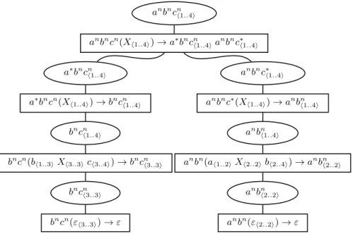
If we use this PRCG to parse the DAG of Figure 1 which defines the language {ab, bc}, we (erroneously) get the non-empty parse for-est of Figure 2 though neither ab nor bc is in anbncn.6 It is not difficult to see that the problem comes from the non-linear instantiated variable Xh1..4i in the start node, and more precisely from the actual (wrong) meaning of the three differ-ent occurrences of Xh1..4i in anbncn(Xh1..4i) → a∗bncn(X
h1..4i) anbnc∗(Xh1..4i). The first occur-rence in its RHS says that there exists a path in the input DAG from state1 to state 4 which is an a∗bncn. The second occurrence says that there exists a path from state 1 to state 4 which is an anbnc∗. While the LHS occurrence (wrongly) says that there exists a path from state1 to state 4 which is an anbncn. However, if the two Xh1..4i’s in the RHS had selected common paths (this is not pos-sible here) between1 and 4, a valid interpretation could have been proposed.
With this example, we see that the difficulty of DAG parsing only arises with non-linear PRCGs.
If we consider linear PRCGs, the sub-class of the PRCGs which is equivalent to LCFRSs, the
6
In this forest oval nodes denote different instantiated predicates, while its associated instantiated clauses are presented as its daughter(s) and are denoted by square nodes. The LHS of each instantiated clause shows the instantiation of its LHS symbols. The RHS is the corresponding sequence of instantiated predicates. The number of daughters of each square node is the number of its RHS instantiated predicates.
standard algorithm works perfectly well with input DAGs, since a valid instantiation of an argument of a predicate in a clause by some range hp..qi means that there exists (at least) one path between p and q which is recognized.
The paper will now concentrate on non-linear PRCGs, and will present a new valid parsing algorithm and study its complexities (in space and time).
In order to simplify the presentation we introduce this algorithm as a post-processing pass which will work on the shared parse-forest output by the (slightly modified) standard algorithm which accepts DAGs as input.
3.2 Parsing DAGs with non-linear PRCGs
The standard parsing algorithm of (Boullier, 2004) working on a string w can be sketched as follows. It uses a single memoized boolean function predicate(A, ~ρ) where A is a predicate and ~ρ is a vector of ranges whose dimension is arity(A). The initial call to that function has the form predicate (S, h0..|w|i). Its purpose is, for each A0-clause, to instantiate each of its symbols in a consistant way. For example if we assume that the ithargument of
the LHS of the current A0-clause is α′iXaY α′′i and that the ithcomponent of ~ρ0is the rangehpi..qii an
instantiation of X, a an Y by the rangeshpX..qXi, hpa..qai and hpY..qYi is such that we have pi ≤ pX ≤ qX = pa < qa= pa+ 1 = pY ≤ qY ≤ qi and w= w′aw′′with|w′| = pa. Since the PRCG is non bottom-up erasing, the instantiation of all the LHS symbols implies that all the arguments of the RHS predicates Ai are also instantiated and gathered into the vector of ranges ~ρi. Now, for each i (1 ≤ i ≤ |RHS|), we can call predicate (Ai, ~ρi). If all these calls succeed, the instantiated clause can be stored as a component of the shared parse forest.7
In the case of a DAG D = (Q, Σ, δ, q0, F) as input, there are two slight modifications, the ini-tial call is changed by the conjunctive call pred-icate(S, hq0..f1i) ∨ . . . ∨ predicate (S, hq0..f|F |i) with fi∈ F8and the terminal symbol a can be in-stantiated by the rangehpa..qaiDonly if(pa, a, qa)
7Note that such an instantiated clause could be
unreachable from the (future) instantiated start symbol which will be the axiom of the shared forest considered as a CFG.
8
Technically, each of these calls produces a forest. These individual forests may share subparts but their roots are all different. In order to have a true forest, we introduce a new root, the super-root whose daughters are the individual forests.
anbncn h1..4i anbncn(Xh1..4i) → a∗bncnh1..4ia n bnc∗h1..4i a∗bncn h1..4i a∗bncn(X h1..4i) → bncnh1..4i anbnc∗ h1..4i anbnc∗(X h1..4i) → anbnh1..4i bncn h1..4i bncn(b
h1..3iXh3..3ich3..4i) → bncnh3..3i
anbn h1..4i
anbn(a
h1..2iXh2..2ibh2..4i) → anbnh2..2i
bncn h3..3i bncn(ε h3..3i) → ε anbn h2..2i anbn(ε h2..2i) → ε
Figure 2: Parse forest for the input DAG ab|bc.
is a transition in δ. The variable symbol X can be instantiated by the range hpX..qXiD only if hpX..qXiDis valid.
3.3 Forest Filtering
We assume here that for a given PRCG G we have built the parse forest of an input DAG D as explained above and that each instantiated clause of that forest contains the range hpX..qXiD of each of its instantiated symbols X. We have seen in Example 1 that this parse forest is valid if G is linear but may well be unvalid if G is non-linear. In that latter case, this happens because the range hpX..qXiD of each instantiation of the non-linear variable X selects the whole sub-DAG DhpX..qXi while each instantiation should only select a sub-language ofL(DhpX..qXi). For each occurrence of X in the LHS or RHS of a non-linear clause, its sub-languages could of course be different from the others. In fact, we are interested in their intersections: If their intersections are non empty, this is the language which will be associated with hpX..qXiD, otherwise, if their intersections are empty, then the instantiation of the considered clause fails and must thus be removed from the forest. Of course, we will consider that the language (a finite number of strings) associated with each occurrence of each instantiated symbol is represented by a DAG.
The idea of the forest filtering algorithm is to first compute the DAGs associated with each argument of each instantiated predicate during a bottom-up walk. These DAGs are called decorations. This processing will perform DAG compositions (including intersections, as suggested above), and will erase clauses in which empty intersections occur. If the DAG associated with the single argument of the super-root is empty, then parsing failed.
Otherwise, a top-down walk is launched (see below), which may also erase non-valid instantiated clauses. If necessary, the algorithm is completed by a classical CFG algorithm which erase non productive and unreachable symbols leaving a reduced grammar/forest.
In order to simplify our presentation we will assume that the PRCGs are non-combinatorial and bottom-up non-erasing. However, we can note that the following algorithm can be generalized in order to handle combinatorial PRCGs and in particular with overlapping arguments.9 Moreover, we will assume that the forest is non cyclic (or equivalently that all cycles have previously been removed).10
9For example the non-linear combinatorial clause
A(XY Z) → B(XY ) B(Y Z) has overlapping arguments.
3.3.1 The Bottom-Up Walk
For this principle algorithm, we assume that for each instantiated clause in the forest, a DAG will be associated with each occurrence of each instantiated symbol. More precisely, for a given instantiated A0-clause, the DAGs associated with the RHS symbol occurrences are composed (see below) to build up DAGs which will be associated with each argument of its LHS predicate. For each LHS argument, this composition is directed by the sequence of symbols in the argument itself.
The forest is walked bottom-up starting from its leaves. The constraint being that an instantiated clause is visited if and only if all its RHS instantiated predicates have already all been visited (computed). This constraint can be satisfied for any non-cyclic forest.
To be more precise, consider an instantiation cρ = A0( ~ρ0) → A1( ~ρ1) . . . Ap( ~ρp) of the clause c = A0( ~α0) → A1( ~α1) . . . Am( ~αm), we perform the following sequence:
1. If the clause is not top-down linear (i.e., there exist multiple occurrences of the same variables in its RHS arguments), for such variable X let the range hpX..qXi be its instantiation (by definition, all occurrences are instantiated by the same range), we perform the intersection of the DAGs associated with each instantiated predicate argument X. If one intersection results in an empty DAG, the instantiated clause is removed from the forest. Otherwise, we perform the following steps.
2. If a RHS variable Y is linear, it occurs once in the jthargument of predicate Ai. We perform
a brand new copy of the DAG associated with the jthargument of the instantiation of Ai.
3. At that moment, all instantiated variables which occur in cρare associated with a DAG. For each occurrence of a terminal symbol t in the LHS arguments we associate a (new) DAG whose only transition is(p, t, q) where p and q are brand new states with, of course, p < q.
4. Here, all symbols (terminals or variables) are associated with disjoints DAGs. For each LHS argument ~α0[i] = Xi
1. . . Xji. . . Xpii, we associate a new DAG which is the
concatenation of the DAGs associated with the symbols X1, . . . , Xi ji, . . . and Xpii. 5. Here each LHS argument of cρis associated
with a non empty DAG, we then report the individual contribution of cρ into the (already computed) DAGs associated with the arguments of its LHS A0( ~ρ0). The DAG associated with the ith argument of A0( ~ρ0) is
the union (or a copy if it is the first time) of its previous DAG value with the DAG associated with the ithargument of the LHS of cρ.
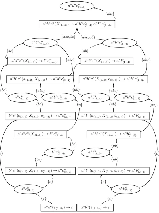
This bottom-up walk ends on the super-root with a final decoration say R. In fact, during this bottom-up walk, we have computed the intersection of the languages defined by the input DAG and by the PRCG (i.e., we haveL(R) = L(D) ∩ L(G)). Example 2. 1 a 2 3 4 b b c b
Figure 3: Input DAG associated with abc|ab|bc. With the PRCG of Example 1 and the input DAG of Figure 3, we get the parse forest of Figure 4 whose transitions are decorated by the DAGs computed by the bottom-up algorithm.11 The crucial point to note here is the intersection which
is performed between{abc, bc} and {abc, ab} on anbncn(Xh1..4i) → a∗bncnh1..4ianbnc∗h1..4i . The non-empty set{abc} is the final result assigned to the instantiated start symbol. Since this result is non empty, it shows that the input DAG D is rec-ognized by G. More precisely, this shows that the sub-language of D which is recognized by G is {abc}.
However, as shown in the previous example, the (undecorated) parse forest is not the forest built for the DAGL(D) ∩ L(G) since it may contain non-valid parts (e.g., the transitions labelled{bc} or {ab} in our example). In order to get the
11
For readability reasons these DAGs are represented by their languages (i.e., set of strings). Bottom-up transitions from instantiated clauses to instantiated predicates reflects the computations performed by that instantiated clause while bottom-up transitions from instantiated predicates to instantiated clauses are the union of the DAGs entering that instantiated predicate.
anbncnh1..4i anbncn(X h1..4i) → a∗bncnh1..4ia nbnc∗ h1..4i a∗bncn h1..4i a∗bncn(X h1..4i) → bncnh1..4i a∗bncn(a
h1..2iXh2..4i) → a∗bncnh2..4i
anbnc∗ h1..4i
anbnc∗(X
h1..4i) → anbnh1..4i
anbnc∗(X
h1..3ich3..4i) → anbnc∗h1..3i
bncnh1..4i
bncn(b
h2..3iXh3..3ich3..4i) → bncnh3..3i
a∗bncnh2..4i
a∗bncn(X
h2..4i) → bncnh2..4i
anbnh1..4i
anbn(a
h1..2iXh2..2ibh2..4i) → anbnh2..2i
anbnc∗h1..3i anbnc∗(X h1..3i) → anbnh1..3i bncn h3..3i bncn(ε h3..3i) → ε bncn h2..4i
bncn(bh2..3iXh3..3ich3..4i) → bncnh3..3i
anbn h2..2i anbn(ε h2..2i) → ε anbn h1..3i
anbn(ah1..2iXh2..2ibh2..3i) → anbnh2..2i
{abc}
{abc, bc} {abc, ab}
{bc}
{abc} {ab}
{abc}
{bc} {abc} {ab} {abc}
{bc} {bc} {ab} {ab} {ε} {bc} {ε} {ab} {ε} {bc} {ε} {ab} {ε} {ε}
right forest (i.e., to get a PRCG parser — not a recognizer — which accepts a DAG as input) we need to perform another walk on the previous decorated forest.
3.3.2 The Top-Down Walk
The idea of the top-down walk on the parse forest decorated by the bottom-up walk is to (re)compute all the previous decorations starting from the bottom-up decoration associated with the instantiated start predicate. It is to be noted that (the language defined by) each top-down decoration is a subset of its bottom-up counterpart. However, when a top-down decoration becomes empty, the corresponding subtree must be erased from the forest. If the bottom-up walk succeeds, we are sure that the top-down walk will not result in an empty forest. Moreover, if we perform a new bottom-up walk on this reduced forest, the new bottom-up decorations will denote the same language as their top-down decorations counterpart.
The forest is walked top-down starting from the super-root. The constraint being that an instantiated A(~ρ)-clause is visited if and only if all the occurrences of A(~ρ) occurring in the RHS of instantiated clauses have all already been visited. This constraint can be satisfied for any non-cyclic forest.
Initially, we assume that each argument of each instantiated predicate has an empty decoration, except for the argument of the super-root which is decorated by the DAG R computed by the bottom-up pass.
Now, assume that a top-down decoration has been (fully) computed for each argument of the instantiated predicate A0( ~ρ0). For each instantiated clause of the form cρ = A0( ~ρ0) → A1( ~ρ1) . . . Ai(~ρi) . . . Am( ~ρm), we perform the following sequence:12
1. We perform the intersection of the top-down decoration of each argument of A0( ~ρ0) with the decoration computed by the bottom-up pass for the same argument of the LHS predicate of cρ. If the result is empty, cρ is erased from the forest.
2. For each LHS argument, the previous results are dispatched over the symbols of this
12The decoration of each argument of A
i( ~ρi) is either
initially empty or has already been partially computed.
argument.13 Thus, each instantiated LHS symbol occurrence is decorated by its own DAG. If the considered clause has several occurrences of the same variable in the LHS arguments (i.e., is bottom-up non-linear), we perform the intersection of these DAGs in order to leave a single decoration per instantiated variable. If an intersection results in an empty DAG, the current clause is erased from the forest.
3. The LHS instantiated variable decorations are propagated to the RHS arguments. This propagation may result in DAG concatena-tions when a RHS argument is made up of several variables (i.e., is combinatorial). 4. At last, we associate to each argument
of Ai(~ρi) a new decoration which is computed as the union of its previous top-down decoration with the decoration just computed.
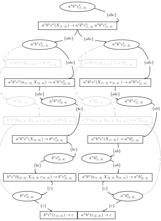
Example 3. When we apply the previous al-gorithm to the bottom-up parse forest of Exam-ple 2, we get the top-down parse forest of Fig-ure 5. In this parse forest, erased parts are laid out in light gray. The more noticable points w.r.t. the bottom-up forest are the decorations be-tween anbncn(Xh1..4i) → a∗bncn
h1..4ia nbnc∗
h1..4i and its RHS predicates a∗bncn
h1..4i and anbnc∗h1..4i which are changed both to{abc} instead of {abc, bc} and {abc, ab}. These two changes induce the indicated erasings.
13
Assume that ~ρ0[k] = hp..qiD, that the decoration DAG
associated with the kth argument of A0( ~ρ0) is Dhp..qi′ =
(Q′
hp..qi,Σhp..qi, δhp..qi′ , p′, Fhp..qi′ ) (we have L(D′hp..qi) ⊆
L(Dhp..qi)) and that ~α0[k] = α1kXα2kand thathi..jiDis the
instantiation of the symbol X in cρ. Our goal is to extract
from D′hp..qi the decoration DAG D′hi..ji associated with
that instantiated occurrence of X. This computation can be helped if we maintain, associated with each decoration DAG a function, say d, which maps each state of the decoration DAG to a set of states (bounds) of the input DAG D. If, as we have assumed, D is minimal, each set of states is a singleton, we can write d(p′) = p, d(f′) = q for all f′ ∈ F′
hp..qi
and more generally d(i′) ∈ Q if i′ ∈ Q′. Let I′ = {i′ |
i′ ∈ Q′
hp..qi∧ d(i′) = i} and J′ = {j′ | j′ ∈ Q′hp..qi∧
d(j′) = j}. The decoration DAG D′
hi..ji is such that
L(D′ hi..ji) =
S
i′∈I′,j′∈J′{x | x is a path from i
′to j′}.
Of course, together with the construction of Dhi..ji′ , its associated function d must also be built.
anbncnh1..4i anbncn(X h1..4i) → a∗bncnh1..4ia nbnc∗ h1..4i a∗bncn h1..4i a∗bncn(X h1..4i) → bncnh1..4i a∗bncn(a
h1..2iXh2..4i) → a∗bncnh2..4i
anbnc∗ h1..4i
anbnc∗(X
h1..4i) → anbnh1..4i
anbnc∗(X
h1..3ich3..4i) → anbnc∗h1..3i
bncnh1..4i
bncn(b
h2..3iXh3..3ich3..4i) → bncnh3..3i
a∗bncnh2..4i
a∗bncn(X
h2..4i) → bncnh2..4i
anbnh1..4i
anbn(a
h1..2iXh2..2ibh2..4i) → anbnh2..2i
anbnc∗h1..3i anbnc∗(X h1..3i) → anbnh1..3i bncn h3..3i bncn(ε h3..3i) → ε bncn h2..4i
bncn(bh2..3iXh3..3ich3..4i) → bncnh3..3i
anbn h2..2i anbn(ε h2..2i) → ε anbn h1..3i
anbn(ah1..2iXh2..2ibh2..3i) → anbnh2..2i
{abc} {abc} {abc} ∅ {abc} ∅ {abc} ∅ {abc} ∅ {abc} ∅ {bc} ∅ {ab} ∅ {bc} ∅ {ab} {ε} {bc} {ε} {ab} {ε} {ε}
3.4 Time and Space Complexities
In this Section we study the time and size complexities of the forest filtering algorithm.
Let us consider the sub-DAG Dhp..qi of the minimal input DAG D and consider any (finite) regular language L ⊆ L(Dhp..qi), and let DL be the minimal DAG s.t. L(DL) = L. We show, on an example, that|DL| may be an exponential w.r.t. |Dhp..qi|.
Consider, for a given h > 0, the language (a|b)h. We know that this language can be represented by the minimal DAG with h+ 1 states of Figure 6.
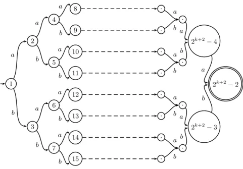
Assume that h = 2k and consider the sub-language L2k of (a|b)2k (nested well-parenthesized strings) which is defined by
1. L2= {aa, bb} ;
2. k >1, L2k = {axa, bxb | x ∈ L2k−2}, It is not difficult to see that the DAG in Figure 7 defines L2kand is minimal, but its size 2k+2− 2 is an exponential in the size2k + 1 of the minimal DAG for the language(a|b)2k.
This results shows that, there exist cases in which some minimal DAGs D′ that define sub-languages of minimal DAGs D may have a exponential size (i.e., |D′| = O(2|D|). In other words, when, during the bottom-up or top-down walk, we compute union of DAGs, we may fall on these pathologic DAGs that will induce a combinatorial explosion in both time and space.
3.5 Implementation Issues
Of course, many improvements may be brought to the previous principle algorithms in practical implementations. Let us cite two of them. First it is possible to restrict the number of DAG copies: a DAG copy is not useful if it is the last reference to that DAG.
We shall here develop the second point on a little more: if an argument of a predicate is never used in an clause involving non-linearity, it is only a waste of time to compute its decoration. We say that Ak, the kth argument of the predicate A
is a non-linear predicate argument if there exists a clause c in which A occurs in the RHS and whose kth argument has at least one common
variable another argument Bh of some predicate B of the RHS (if B = A, then of course k and h must be different). It is clear that Bh is then
non-linear as well. It is not difficult to see that decorations needs only to be computed if they are associated with a non-linear predicate argument. It is possible to compute those non-linear predicate arguments statically (when building the parser) when the PRCG is defined within a single module. However, if the PRCG is given in several modules, this full static computation is no longer possible. The non-linear predicate arguments must thus be identified at parse time, when the whole grammar is available. This rather trivial algorithm will not be described here, but it should be noted that it is worth doing since in practice it prevents decoration computations which can take an exponential time.
4 Conclusion
In this paper we have shown how PRCGs can handle DAGs as an input. If we consider the linear PRCG, the one equivalent to LCFRS, the parsing time remains polynomial. Moreover, input DAGs necessitate only rather cosmetic modifications in the standard parser.
In the non-linear case, the standard parser may produce illegal parses in its output shared parse forest. It may even produce a (non-empty) shared parse forest though no sentences of the input DAG are in the language defined by our non-linear PRCG. We have proposed a method which uses the (slightly modified) standard parser but prunes, within extra passes, its output forest and leaves all and only valid parses. During these extra bottom-up and top-down walks, this pruning involves the computation of finite languages by means of concatenation, union and intersection operations. The sentences of these finite languages are always substrings of the words of the input DAG D. We choose to represent these intermediate finite languages by DAGs instead of sets of strings because the size of a DAG is, at worst, of the same order as the size of a set of strings but it could, in some cases, be exponentially smaller.
However, the time taken by this extra pruning pass cannot be guaranteed to be polynomial, as expected from previously known complexity results (Bertsch and Nederhof, 2001). We have shown an example in which pruning takes an exponential time and space in the size of D. The deep reason comes from the fact that if L is a finite (regular) language defined by some minimal DAG D, there are cases where a sub-language of
0 1 2 h− 1 h a b a b a b
Figure 6: Input DAG associated with the language(a|b)h, h >0.
1 2 3 4 5 6 7 8 9 10 11 12 13 14 15 . . . . . . . . . . . . 2k+2− 4 2k+2− 3 2k+2− 2 a b a b a b a b a b a b a b a b a b a b a b a b a b a b
Figure 7: DAG associated with the language of nested well-parenthesized strings of length2k.
L may require to be defined by a DAG whose size is an exponential in the size of D. Of course this combinatorial explosion is not a fatality, and we may wonder whether, in the particular case of NLP it will practically occur?
References
Franois Barth´elemy, Pierre Boullier, Philippe
De-schamp, and ´Eric de la Clergerie. 2001. Guided
parsing of range concatenation languages. In
Pro-ceedings of the 39th Annual Meeting of the Associ-ation for Comput. Linguist. (ACL’01), pages 42–49,
University of Toulouse, France.
Eberhard Bertsch and Mark-Jan Nederhof. 2001. On the complexity of some extensions of rcg parsing. In
Proceedings of IWPT’01, Beijing, China.
Pierre Boullier, 2004. New Developments in
Pars-ing Technology, volume 23 of Text, Speech and Language Technology, chapter Range
Concatena-tion Grammars, pages 269–289. Kluwer Academic Publishers, H. Bunt, J. Carroll, and G. Satta edition.
Jeffrey D. Hopcroft and John E. Ullman. 1979.
Introduction to Automata Theory, Languages, and Computation. Addison-Wesley, Reading, Mass.
Bernard Lang. 1994. Recognition can be harder than
parsing. Computational Intelligence, 10(4):486–
494.
K. Vijay-Shanker, David Weir, and Aravind K. Joshi. 1987. Characterizing structural descriptions produced by various grammatical formalisms. In
Proceedings of the 25th Meeting of the Association for Comput. Linguist. (ACL’87), pages 104–111,