An acoustic sensor for measuring traffic variables

An Acoustic Sensor for Measuring Traffic

Variables

by

Ramona Hui Tung

Submitted to the Department of Electrical Engineering and

Computer Science

in partial fulfillment of the requirements for the degree of

Master of Science in Electrical Engineering

at the

MASSACHUSETTS INSTITUTE OF TECHNOLOGY

September 1994

@

Massachusetts Institute of Technology 1994. All rights reserved.

A uthor ...

Department of Electrical Engineering and Computer Science

.T1nm A 1 .4

Certified by...

James K. Roberge

Professor of Electrical Engineering

Thesis Supoprvisor

Certified by...

V

Antnony k.

Hotz

Off-Campus Supervisor

/-) The•iq SRnnmrvisor

Accepteidy ...

SQ

X),

·'C~

-Chairman,

Srreueric

~yiorgentniaer

An Acoustic Sensor for Measuring Traffic Variables

by

Ramona Hui Tung

Submitted to the Department of Electrical Engineering and Computer Science on June 6, 1994, in partial fulfillment of the

requirements for the degree of Master of Science in Electrical Engineering

Abstract

The Intelligent Vehicle-Highway System (IVHS) program requires a large number of sensors to accurately measure traffic data. A novel passive acoustic sensing scheme based upon a triple-aperture microphone array is proposed as an inexpensive, reliable alternative to other sensors under consideration. A single sensor exhibits the potential for monitoring several lanes of traffic simultaneously. An algorithm for determining vehicle speed and range from the microphone outputs is discussed and directions for future research are identified.

Thesis Supervisor: James K. Roberge Title: Professor of Electrical Engineering Thesis Supervisor: Anthony F. Hotz Title: Off-Campus Supervisor

Acknowledgments

I would like to thank the MIT Lincoln Laboratory and Group 76 for their continual support of my work over the last four years (the last two of which were devoted to the research for this thesis). Special thanks go to Tony Hotz and Rob Gilgen who first suggested the use of microphones for traffic sensing, to Professor James K. Roberge, Dr. Richard Lacoss, and Professor Amar G. Bose who always made available their technical expertise and suggestions, and to Lenny Lopez who went above and beyond the call of duty to make sure the experimental work ran smoothly.

I am deeply indebted to Carl Much, the leader of Group 76, who consistently went out of his way to insure that I had everything I needed. I doubt that I will ever meet a more caring and supportive technical manager. I am also especially grateful to Tony Hotz for providing insight and intellectual stimulation (and exasperation...) in all areas (and for putting up with me as his first, and probably last, thesis student for the past two years). In addition, I would like to thank all the members of Group 76 (current and former) whose friendship and encouragement made working at Lincoln a real pleasure.

Last, but not least, I would like to thank my family and friends for believing in me. And finally, thanks to Avi, for giving me an incentive to finish...

Contents

1 Vehicle Sensing 10

1.1 O bjectives . . . .. . 10

1.2 Current Sensing Options ... .. 10

1.2.1 Continuous Sensors ... . . .. 11

1.2.2 Discrete Sensors ... ... .... ... .... .. 11

1.3 Proposed Sensing Scheme ... . . . . . 13

2 Sensor Components 15 2.1 O verview . . . .. . 15

2.2 M icrophones ... ... 16

2.2.1 Audible Range Microphones . ... 17

2.2.2 Ultrasonic Microphones ... 20 2.3 Accelerometers ... ... .. ... 21 2.4 Am plifiers . . . .. . . .. . . .. .. . .. .. . . . .. . 24 3 Experimental Procedure 26 3.1 Test Plan ... ... .. 26 3.2 Controlled Experiments ... 27

3.2.1 Field Test One ... .. ... . 28

3.2.2 Field Test Two ... . ... ... ... .. 39

3.2.3 Field Test Three .... ... ... ... . 43

3.3 Road Tests ... .... .. . . 46

3.3.2 Road Test Two ... 53

3.3.3 Road Test Three ... 54

4 Sensor Algorithm 60 4.1 Basic Theory ... 60

4.2 Time Delay Estimation ... 60

4.3 Block Diagram of Algorithm ... .... 62

4.4 Speed Estimation ... 68

4.5 Range Estimation ... 70

4.5.1 Localization with Hyperbolic RDL . ... 70

4.5.2 Range Determination Using the LOCA Technique ... 72

4.5.3 Source Tracking With the Extended Kalman Filter ... 78

4.6 M ultiple Vehicles ... 79

4.7 Algorithm Performance ... 92

4.8 Sensor Design Issues ... 94

4.8.1 Hardware Considerations ... ... 94 4.8.2 Algorithm Parameters ... ... 96 5 Conclusions 102 5.1 Future W ork ... 102 5.2 Sum m ary . . . .. . . . .. . .. . . . . . . . ... . .. 104 A Acoustic Identifiers 107 B Circuit Diagrams 109 C Verification System 115 D Alternative Algorithm Approaches 122 D.0.1 Short-Term Fourier Transforms . ... 122

List of Figures

2-1 Photograph of microphones used to collect traffic data ... . . 18

2-2 Frequency response of Radio Shack 270-090 microphones ... 19

2-3 Frequency response of Sennheiser KE 10-420 microphones . ... 19

2-4 Photograph of accelerometers used to collect traffic data ... 22

2-5 Frequency response of Analog Devices ADXL50 accelerometer . . .. 23

2-6 Block diagram of AC amplifier design . ... 24

2-7 Photograph of amplifier module ... ... . . . 25

3-1 Approximate frequency response of the analog recorder ... 28

3-2 Experimental configuration for Field Test One . ... 29

3-3 Microphone assembly for Field Test One . ... 31

3-4 Microphone mounting boxes . ... .... 32

3-5 Accelerometer measurement axes for Field Test One ... . . . . . 33

3-6 Spectrum of the Subaru XT6 as measured by a Radio Shack microphone 34 3-7 Spectrum of the Subaru XT6 as measured by an ultrasonic microphone 35 3-8 7- vs. time for the Subaru XT6 . ... . .. 36

3-9 Separated curves for acoustic sources in front and rear of Subaru XT6 37 3-10 Microphone assembly for Field Test Two . ... 40

3-11 T vs. time plot for pickup truck passing array at 30 ft ... 42

3-12 Spectrum of vehicle coasting by in neutral (snapshot) . ... 45

3-13 A T vs. time plot obtained from a vehicle coasting by in neutral . . . 46

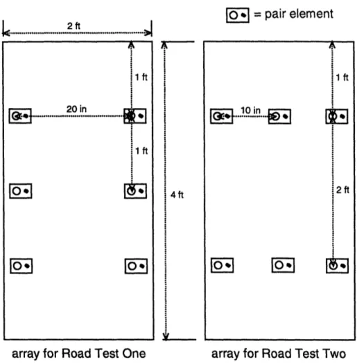
3-14 Experimental configuration for Road Test One . ... 48

3-16 3-17 3-18 3-19 3-20 3-21 3-22 4-1 4-2 4-3 4-4

Microphone arrays for Road Test One and Two . . . . . Low frequency microphone assembly . . . .

A typical time domain plot from an ultrasonic sensor . . Experimental configuration for Road Test Two . . . . Photograph of microphone assembly for Road Test Two . Microphone configuration for Road Test Three . . . . Experimental configuration for Road Test Three . . . . . Block diagram of current algorithm . . . . A sample theoretical T vs. time curve . . . . A r- vs. time plot obtained from a pair of microphones . Geometry of vehicle tracking problem . . . .

. . . . . 5 1 . . . . . 52 . . . . . 53 . . . . . 56 . . . . . 57 . . . . . 58 . . . . . 59 . . . . . 64 . . . . . 65 . . . . . 67 . . . . . 69 4-5 Typical microphone configuration used with the LOCA algorithm . .

4-6 A basic trajectory shape returned by LOCA when the theoretical T

values are offset . . . . 4-7 Another basic trajectory shape returned by LOCA when the theoretical

-_{values are offset . . . .}

4-8 Ry _{returned by LOCA for single triads (focus) vs. two triads}

(inter-section) . . . . 4-9 7 vs. time for two vehicles crossing from opposite directions .. . . .

4-10 Separated curves for two vehicles crossing from opposite directions . .

4-11 T vs. time for two vehicles crossing from opposite directions .. . . .

4-12 Separated curves for two vehicles crossing from opposite directions . .

4-13 7 _{vs. time for two vehicles following each other closely} .. . . .

4-14 Separated curves for two vehicles following each other closely... 4-15 7- _{vs. time for a car in lane 3 overtaking a semi in lane 4 (Case 1) .}

4-16 Separated curves for car overtaking semi (Case 1) .. . . .

4-17 T _{vs. time for a car in lane 3 overtaking a semi in lane 4 (Case 2) .} .

4-18 Separated curves for car overtaking semi (Case 2) .. . . .

B-1 Circuit diagram for Radio Shack microphone amplifier ... . 110

B-2 Circuit diagram for Sennheiser microphone amplifier ... 111

B-3 Circuit diagram for ADXL50 accelerometer amplifier . ... 112

B-4 Circuit diagram for Murata-Erie ultrasonic microphone amplifier . . . 113

B-5 Circuit diagram for anti-aliasing filter . ... 114

C-1 Debounce PAL finite state machine . ... 117

C-2 Control PAL finite state machine . ... . 118

C-3 Diagram of the debounce circuit for Field Test One . ... 119

C-4 Diagram of the verification control circuit for Field Test One ... 120 C-5 Photograph of hardware for the verification system of Field Test One 121

List of Tables

4.1 Algorithm speed estimates for multiple vehicle cases ... 92 4.2 Algorithm speed estimates for single vehicle cases . ... 93

Chapter 1

Vehicle Sensing

1.1

Objectives

Broadly stated, the proposed Intelligent Vehicle-Highway System (IVHS) is a national program which will use advanced technology to help solve transportation problems and improve safety. For example, some strategies for congestion management will attempt to optimize traffic flow by providing dynamic route guidance to vehicles based upon advance destination information from individual vehicles and real-time information from roadway sensors. Many sensors will be required for such applications and in order to minimize the cost of IVHS, low-cost sensors are desirable. Moreover, the sensors should be durable, require little maintenance, and remain insensitive to variable illumination, weather, and road conditions. However, they must provide accurate and reliable traffic information. Some important traffic data which must be measured includes detection of passing vehicles, vehicle location (lane determination), vehicle speed, and vehicle class.

1.2

Current Sensing Options

Sensing schemes currently under consideration for IVHS applications include visible and infrared video, "dead reckoning" (using the Global Positioning Satellite network), passive inductive (using buried loop detectors), ultrasonic, vehicle transponder, and

passive acoustic systems[3] [6]. These can be loosely subdivided into "continuous" and "discrete" sensors. The advantages and disadvantages of each of these is discussed

briefly.

1.2.1

Continuous Sensors

"Continuous" sensors, which include video, infrared, and "dead reckoning" systems, are capable of monitoring long stretches of road with a single sensor. Through sophis-ticated image processing algorithms, visible light video systems detect and classify vehicles, as well as measure speed and estimate queue lengths. However, their ac-curacy and reliability is often hampered by poor lighting and weather conditions (fog, rain, snow). Alternatively, infrared cameras, which are relatively insensitive to variable lighting and weather conditions, can perform similar functions, but the con-siderable expense for cryogenic cooling makes them unattractive. Uncooled infrared arrays are under development and prototypes exist, but they remain more costly than most other sensors under consideration. A "dead reckoning" system would use the Global Positioning Satellite (GPS) network to report a vehicle's exact location. Such a system would be extremely accurate but would require each vehicle to be equipped with GPS or cellular communication equipment, thus putting a large share of the system cost on the users. In addition, an efficient communications link would be re-quired for handling vehicle position reports. For many IVHS applications, it is more important to monitor traffic flow patterns rather than individual vehicles. Since the GPS network provides a higher level of precision than is necessary, it seems more practical to use a simpler, cheaper sensing system.

1.2.2

Discrete Sensors

"Discrete" sensors, which include passive inductive, ultrasonic, vehicle transponder, and passive acoustic systems, obtain traffic data by considering individual vehicles. Passive inductive systems use buried inductive loops to count passing vehicles. A pair of inductive loops closely spaced can also supply speed information. In contrast,

mounted above the roadway, ultrasonic sensors measure reflections of transmitted signals from a vehicle passing beneath the sensor to get estimates of vehicle height and length for classification. Vehicle speed is determined by measuring the Doppler velocity of the moving target. In vehicle transponder systems, vehicles are equipped with "transponders" that respond with a coded reply when a coded signal from an "interrogator" is received. The interrogator then measures the response delay and Doppler shift to determine range and speed. Additional information can be coded into the reply message, making transponders attractive for a wide range of IVHS applications from automating toll collection to providing driver information. Passive acoustic systems extract vehicle information from the outputs of microphone arrays directed toward the traffic. These outputs are correlated and processed to estimate parameters such as speed, range, bearing, and direction of travel.

An important issue for "discrete" sensors is cost (for the sensors, installation, and maintenance) since a large number of closely-spaced sensors are required to monitor traffic flow. Although presently widely used, inductive loops are expensive to install and maintain because they are large and must be buried. Most likely, for IVHS ap-plications they will be augmented with other less expensive sensors. In an ultrasonic sensing scheme, the active transmitters consume power. Furthermore, the sensors require costly overhead mounting structures for installation. In vehicle transponder systems, the cost is shared between the traffic control system (interrogators and pro-cessors) and the users (transponders). Because the interrogators are active and the transponders can be either active' or passive2_{, there will be some power requirements.}

Moreover, the high frequency radiation from the interrogators may raise health issues from the general public. Placement of the interrogators also requires consideration. The possibilities, which include mounting them overhead, building "toll booth"-like structures to house them, or burying them in the road, could be quite expensive.

Alternatively, passive acoustic systems, which are among the newest of the pro-posed sensing schemes, are of interest because the sensing elements are microphones

'By sending a digital message

2

which are inexpensive and widely available. In addition, the sensor package could be installed at the side of the road with minimal effort and equipment, which facil-itates servicing. Conceivably, a sensing scheme which tracks vehicles with an array of closely-spaced microphones would prove an inexpensive, reliable, low-maintenance alternative to the methods mentioned earlier.

1.3

Proposed Sensing Scheme

This thesis explores the development of a passive acoustic sensor based upon a triple-aperture microphone array. The microphone outputs are correlated to estimate the delays (which will be denoted by 7) between the time a source signal is received at one microphone relative to the next. From the geometry of the problem, if the delay estimates are accurate enough, a vehicle's position and speed can be determined. Methods for improving the accuracy of the 7 estimates and for removing biases in range and bearing estimates obtained from noisy delay estimates can be found in many underwater signal processing texts such as the one by Joseph C. Hassab [2].

When the proposal for this thesis was submitted on February 9, 1993, a literature search conducted at the MIT Lincoln Laboratory had not turned up any articles men-tioning the use of microphones in vehicle sensing schemes. However, in April of 1993, AT&T announced it was developing a passive acoustic sensor (the SmartSonicTM TSS) using technology from anti-submarine warfare research [4] [5]. Their sensor is

based upon an array of 60 microphones in a package the size of a pizza box which is mounted overhead on existing fixtures along the side of the road. Using beamforming techniques, the sensor focuses on a 10' x 6' section of road (i.e.. one lane) and moni-tors the traffic flow through this square, concentrating on the frequency range from 4 to 6 kHz. It provides accurate traffic counts and occupancy for the lane under surveil-lance and is able to distinguish between larger vehicles (such as trucks and buses) and automobiles.3 At the present time, AT&T is trying to expand the capabilities of its sensor to monitor two lanes and provide vehicle classification. Currently, the

sensor is reported to cost around $2000.

In contrast, the passive acoustic sensor proposed in this thesis is composed of "off the shelf" components and primarily uses simple correlation techniques for process-ing. Experimental results indicate that the proposed sensor is capable of monitoring traffic simultaneously in both directions on a road with a single lane of travel in each direction. It further suggests that with additional processing, a single sensor will be able to monitor roads with multiple lane traffic in both directions. This issue will be pursued in the future. Vehicle classification has not been examined closely, but seems feasible with further processing. The potential of this passive acoustic scheme combined with its low cost make it an idea worth developing and considering as a viable alternative for IVHS applications.

Chapter 2

Sensor Components

2.1

Overview

The sensor package, which is installed at the side of the road a few feet off the ground, consists of an array of three microphones' and associated processing hardware. The outputs of the microphones are first amplified and bandpass-filtered before being digitized for processing. Processor architecture has not been investigated in detail, but is expected to be simple and inexpensive since current algorithms require only basic operations.

The use of accelerometers to detect vehicle vibration through the road bed was also explored but ultimately rejected. It was hypothesized that road vibration patterns could be analyzed to extract source vehicle information. To minimize transmission loss, accelerometers were glued to circular aluminum disks which were attached di-rectly to the road surface with long carpentry nails. Unfortunately, the accelerometers used, which were quite sensitive, did not pick up any ground vibration at all. Seismic accelerometers, which are ten times more sensitive, are available but too expensive to consider. In retrospect, it appears unlikely that accelerometers would provide any in-formation not obtainable from processing microphone outputs. Nevertheless, because they were a key component in the initial design, accelerometers will be included in

the description of the sensor design and evaluation phases.

2.2

Microphones

In the design of the passive acoustic traffic sensor, both ultrasonic and audible range microphones were considered. The current sensor algorithm depends solely on the outputs of audible range microphones. Nonetheless, data was collected from both types of microphones to allow development of future algorithms which might incor-porate ultrasonic sensor outputs for improved accuracy and reliability. The benefits and disadvantages of each type of microphone are discussed briefly below.

It has been found that correlating the outputs of audible range microphones yields reliable speed estimates for relatively low sampling rates when the signal-to-noise ratio (SNR) is high. The fact that these microphones are inexpensive and widely available makes them even more interesting for IVHS applications. The main concern over audible range microphones is their sensitivity to a wide variety of background noise which could corrupt measurements. Some form of active filtering might be required for robustness in low SNR cases.

On the other hand, ultrasonic microphones (with a frequency range from 15-30 kHz) are attractive because they are especially sensitive to tire/road interface noise yet insensitive to most background noise. The drawbacks are that they are slightly more expensive, not as readily available, and require higher initial sampling rates and more sophisticated processing techniques. Yet ultrasonic microphones are worth examining because of the push in the automotive industry toward designing quieter vehicles. If electric cars ever become popular, vehicles will be virtually silent. Quiet vehicles may present difficulties for sensing systems focusing on audible emissions. However, ultrasonic microphones do not face this problem due to their sensitivity to tire/road interface noise. No matter how silent a vehicle is, as long as it has wheels it remains detectable by ultrasonic microphones.

2.2.1

Audible Range Microphones

A wide variety of microphones are commercially available for all types of acoustic applications. A number of criteria were considered in the selection of a suitable audible range microphone:

1. Cost 2. Bandwidth 3. Sensitivity

4. Flatness of its frequency response

5. Directivity (directional vs. omnidirectional)

Because the IVHS program will require large numbers of reliable traffic sensors, an inexpensive, sensitive microphone with a flat frequency response was sought. Fur-thermore, a wide bandwidth was desired because at the time, frequencies of interest had not been determined. Finally, directional (cardioid) microphones were preferred over omnidirectional microphones since the spatial region of interest (i.e., the road) lies directly in front of the array. Omnidirectional microphones introduce noise from other directions which would degrade performance.

On the basis of these criteria, two audible range microphones were selected. The first was a general-purpose omnidirectional electret microphone from Radio Shack (catalog

#

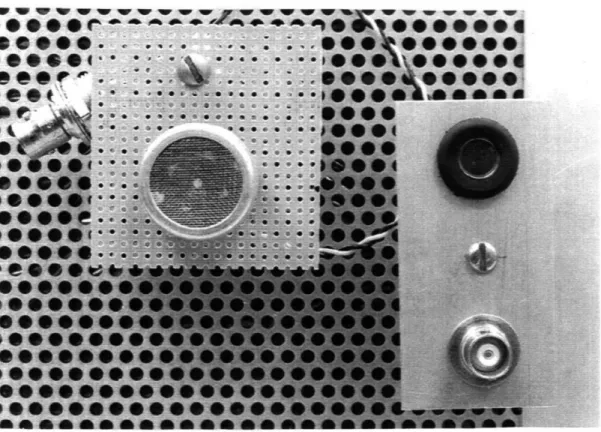
270-090) shown on the left in Figure 2-1. This choice was based largely upon cost and immediate availability. The microphone proved fairly sensitive, al-though it was completely uncalibrated. The obscure frequency response curve which accompanied the sensor appears in Figure 2-2. Consequently, it was only used in a series of controlled tests to collect preliminary data. The second microphone was a low-cost, cardioid microphone from Sennheiser (model # KE 10-420) depicted on the right in Figure 2-1. As reflected by its frequency response curve in Figure 2-3, it meets the high sensitivity, wide bandwidth, and flat response requirements fairly well. These microphones were used to obtain traffic data from an actual road. Sensor

algorithm development and evaluation were conducted primarily with data from the Sennheiser microphones.

Figure 2-1: Photograph of microphones used to collect traffic data

80 dB

70 dB

60 dB

50 dB

Typical Frequency Response

I MM,,MNMMMMý

20 Hz 50

190 200 Hz 500 1000 2000 Hz 500010000 20000

Figure 2-2: Frequency response of Radio Shack 270-090 microphones

KE 10-420

Figure 2-3: Frequency response of Sennheiser KE 10-420 microphones

dB 50 40

10

2.2.2

Ultrasonic Microphones

There are several motivations behind the strong interest in ultrasonic microphones. Initially, they were considered in conjunction with the idea of tagging vehicles with acoustic identifiers (which is described in Appendix A). Likewise, there was specula-tion regarding the possibility of ultrasonic emissions from engine components. More-over, from a signal processing standpoint, since the amount of ultrasonic background noise is minimal, algorithms focusing on ultrasonic frequencies would likely exhibit superior performance due to higher signal-to-noise ratios (SNR). With these ideas in mind, a low-range ultrasonic microphone whose frequency response overlapped the audible range was sought. Overlap was desired so that potentially interesting frequency bands would not be overlooked.

A survey of the market revealed only a few ultrasonic microphone manufacturers. Chief among these were the producers of precision instrumentation sensors (which were extremely expensive) and the manufacturers of ultrasonic imaging sensors. Most ultrasonic imaging sensors had frequency ranges which were greater than 40 kHz, but luckily, one was found which had a nominal frequency of 23 kHz and a bandwidth of 6 kHz centered about the nominal. This microphone was the Murata-Erie MA23-L3-9 depicted in the center of Figure 2-1. Five samples were procured before the part was discontinued in September 1993.

While examining the output of an ultrasonic microphone with an oscilloscope, some interesting observations were made. It was discovered that they are extremely sensitive to impulsive or abrasive sounds.2 _{This observation indicates that the}

micro-phones should sense tire/road interface noise, although they are just as likely to detect pedestrians. Distinguishing a vehicle from a person is not difficult (see Section 3.2.2). To their advantage the ultrasonic microphones did not appear particularly sensitive to speech, planes, or wind (generated by a fan). All of these are factors which could degrade the performance of audible range microphones.

2

Some examples of impulsive sounds are honking, clapping, coughing, or a door slamming. Abra-sive sounds include scraping, rubbing the hands together, and scuffing the feet.

2.3

Accelerometers

An idea trading session sparked interest in two potential applications of accelerometers in the vehicle sensor. In one instance, accelerometers are directly attached to or embedded in the road bed to measure ground vibration patterns. If sensitive enough to detect ground vibration, they should at least be able to distinguish between large, heavy vehicles (such as trucks and buses) and smaller, lighter ones. In an alternative application, an accelerometer with a frequency range extending down to dc is mounted on a flexible membrane. By measuring air vibration it might theoretically serve as a low frequency "microphone".

There was a large assortment of accelerometers to choose from because of their extensive use in projects conducted at the MIT Lincoln Laboratory. Since signals from ground vibration were expected to be low frequency (up to a few Hz) with small amplitudes, the most sensitive accelerometers available were obtained. Cost was not a factor because sensors could be borrowed for determination of sensitivity requirements. Thus, some calibrated Sundstrand QA700 accelerometers (depicted in the center of Figure 2-4) with a sensitivity of 1 V/g (from dc to 300 Hz) were obtained for use in field tests. Though too expensive for use in an IVHS sensor, the QA700s permitted a qualitative evaluation of the feasibility and practicality of using accelerometers in a vehicle sensing scheme. PCB 336B04 piezoelectric accelerometers (seen on the right in Figure 2-4) with a sensitivity of 100mV/g (from 1 to 2000 Hz), were also placed on the road to collect vibration data. Despite lower sensitivity, they are more suitable for IVHS because of their cost.

For the low frequency "microphone", a lightweight accelerometer was required since it would be attached to a flexible membrane. The new ADXL50 accelerometer chip (displayed on the left in Figure 2-4) from Analog Devices was chosen because it was light, cheap, and able to measure accelerations down to dc. Its frequency response is provided in Figure 2-5.

INCHES

Figure 2-4: Photograph of accelerometers used to collect traffic data (from left: Analog Devices ADXL50, Sundstrand QA700, PCB 336B04)

-6 -9 -12 -15 -18 -21 1 10 100 1k FREQUENCY - Hz

Figure 2-5: Frequency response of Analog Devices ADXL accelerometer I a u, 2

N

0

z

10k

2.4

Amplifiers

The sensitivities of the microphones and accelerometers were enhanced with electronic amplifiers. For the Sundstrand and PCB accelerometers, signal conditioners were already available. However, ac amplifiers were designed and built for the microphones and the ADXL50 accelerometer.

The amplifier designs for the Radio Shack and Sennheiser microphones and the ADXL50 accelerometer exhibit the same structure. A block diagram of the amplifier appears in Figure 2-6. After appropriately powering the sensor, its output is ac coupled, amplified, then bandpass filtered to reduce noise. Circuit diagrams are provided in Appendix B in Figures B-1, B-2, and B-3.

x(t)

y(t)

Figure 2-6: Block diagram of AC amplifier design

An amplifier design for the Murata Erie ultrasonic microphones was provided in the specification sheets. The design was modified slightly to avoid gain/bandwidth problems. The final circuit diagram appears in Appendix B in Figure B-4.

A photograph of one of the amplifier modules appears in Figure 2-7. This hardware realizes the amplifiers for five Sennheiser microphones and five ultrasonic microphones. In the future, all requisite amplifier hardware will be part of the sensor package.

Figure 2-7: Photograph of amplifier module (for 5 Sennheiser and 5 Murata-Erie microphones)

Chapter 3

Experimental Procedure

3.1

Test Plan

To get a sense of the bandwidth and shapes of the signals that would be detected on a real road, data was collected in a series of controlled experiments conducted on an experimental track at the MIT Lincoln Laboratory. The main facility of the MIT Lincoln Laboratory is located on Hanscom Air Force Base in Lexington, MA. Microphones and accelerometers were placed in various positions to detect vehicles traveling at constant speed, accelerating, braking, and honking. Analyzing this data provided insight which led to preliminary algorithm development and the decision to base the sensor on a triple-aperture microphone array. In addition, some general ef-fects from acoustic noise sources such as planes, machinery, wind, and people (talking or walking by) were noted.

Following the controlled experiments, an array of both audible range and ultra-sonic microphones was placed at the edge of the driveway of the MIT Lincoln Labo-ratory annex at 45 Hartwell Avenue to collect real traffic data. Located in Lexington, MA, Hartwell Avenue is one of the main roads that leads to Hanscom Air Force Base. It is a bidirectional roadway with two lanes of traffic on each side. Due to saturation of the audible range microphones on the first day of road testing, a gain stage was removed from their amplifiers and the experiment repeated on another day. In a third road test, the microphone configuration was altered to assess the performance of a

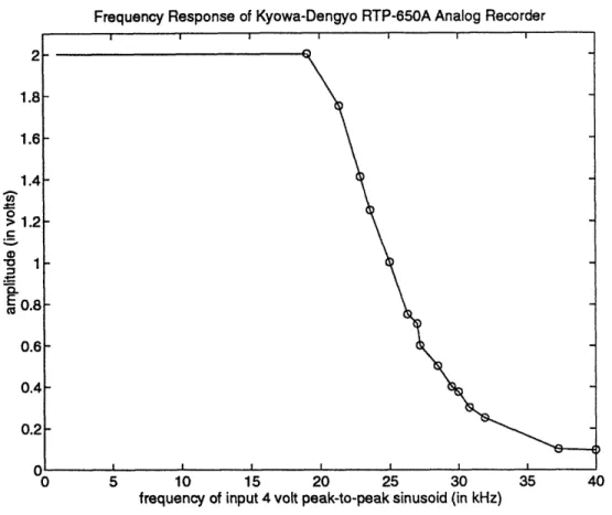
range estimation technique. Traffic was light on all three days during data acquisition. Getting the data into a form which allowed it to be processed required several steps. In all instances, data was stored on beta tapes using a 14-channel Kyowa-Dengyo analog recorder. The recorder had a bandwidth of approximately 20 kHz when set at the fastest recording speed of 76 m. The frequency response of the recorder was gauged by varying the frequency of a 4 volt peak-to-peak sinusoidal input and measuring the amplitude decay. The results are plotted in Figure 3-1. The recorded analog data was passed through an anti-aliasing filter (a Sallen-Key lowpass filter whose circuit diagram appears in Appendix B) before being digitized and stored using Lab Windows running on a PC. In practice, the data acquisition card allowed a maximum total sampling rate (fm,,..) of 85-90 ksps.1 _{In the Lab Windows}

environment, data was viewed and sections selected for conversion to ASCII format. Finally, data analysis and algorithm development were conducted using Matlab.

3.2

Controlled Experiments

Three series of controlled experiments (Field Tests One, Two, and Three) were per-formed and are outlined in this section. The objectives of these tests were to:

1. Identify frequency range(s) of interest

2. Determine the number of sensors needed and suggest their placement 3. Qualitatively assess the sensitivity and range of uncalibrated microphones 4. Provide a starting point for preliminary algorithm development

5. Examine the effects of possible noise sources 6. Start a database for future algorithm development

The experiments performed and insights developed during the three Field Tests are described in the following subsections.

1Since the sampling scheme is multiplexed, the maximum sampling rate per channel is , where N is the number of channels simultaneously sampled.

Frequency Response of Kyowa-Dengyo RTP-650A Analog Recorder

frequency of input 4 volt peak-to-peak sinusoid (in kHz)

Figure 3-1: Approximate frequency response of the analog recorder

3.2.1

Field Test One

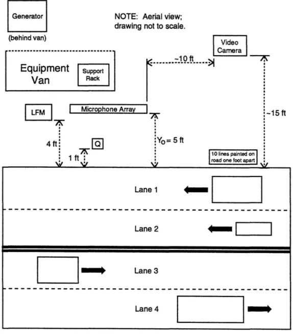
The first field test was conducted in an alley behind the high bay of Building I at the MIT Lincoln Laboratory. The test site was convenient and offered few distractions from other vehicles. The acoustic noise environment that day included some machin-ery noise from the building's ventilation system, light wind in the alley, and a few random noises like doors slamming and people walking. The experimental configura-tion is detailed in the drawing of Figure 3-2. An assortment of sensors were placed along the side of the "road" to collect data.

B

A

Accelerometers

R

SFQ1-1

I

8ft

NOTE: Aerial view;

drawing not to scale.

00

Mounting plates for hoses

Figure 3-2: Experimental configuration for Field Test One

25

ft

Vehicle

Microphones Support Rack

..

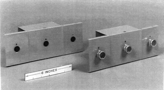
_-;r

-The microphones were placed in the fixtures labeled as A and B in Figure 3-2. Both assemblies had the structure displayed in Figure 3-3. Mounted at the top of a hollow aluminum pole (which provided support) was an 18-inch diameter radar dish-with an omnidirectional Radio Shack microphone at its focal point. The parabolic reflectors were included for two reasons: to make the microphones directional and to determine if their use would greatly improve measurements. Halfway down the pole, three microphones spaced 4 inches apart were positioned on a mounting box (Radio Shack in Assembly A, ultrasonic in Assembly B). The mounting boxes for both arrays are shown in Figure 3-4. The box was attached to the pole using tie wraps. At the base of the assembly was a mount that was attached to the pavement with long carpentry nails.

The verification system used for Field Test One was comprised of a pair of air hoses spaced one meter apart and associated digital circuitry. An air switch at the end of each hose provided a low TTL pulse when a vehicle's wheels ran over the hose. The outputs of the two air switches were routed to the verification circuit which is described in Appendix C. Essentially, each signal is debounced, then fed into a simple finite-state machine which starts a counter when the front wheels cross the hose at A and stops it after they cross the hose at B. Knowing the distance between the hoses and the time it took to cross both of them gives the speed of the vehicle.

Accelerometers were placed in triaxial mounts labeled P (for PCB) and Q (for QA700) in the diagram of Figure 3-2. The mounts were attached to the road with long carpentry nails. The direction of the measurement axes are identified in Figure 3-5. Along with the microphone amplifiers and analog recorder, the signal conditioners for the accelerometers were found on the rack labeled R.

During Field Test One, a vehicle was driven past the sensors at a distance (R,) of about 8 feet. Henceforth, the vertical range component, PR, will denote the perpen-dicular distance between the sensor array and the lane of travel. Several experiments

were conducted, some in which the vehicle was traveling at constant speeds, others where the vehicle was accelerating or braking. A few trials also included the vehicle honking. Two different vehicles, a Subaru XT6 and a Toyota pickup truck, were

Figure 3-3: Microphone assembly for Field Test One

driven for comparison. The primary goals of Field Test One were to identify fre-quency bands of interest and begin a database of basic "traffic" situations to be used for algorithm performance evaluation.

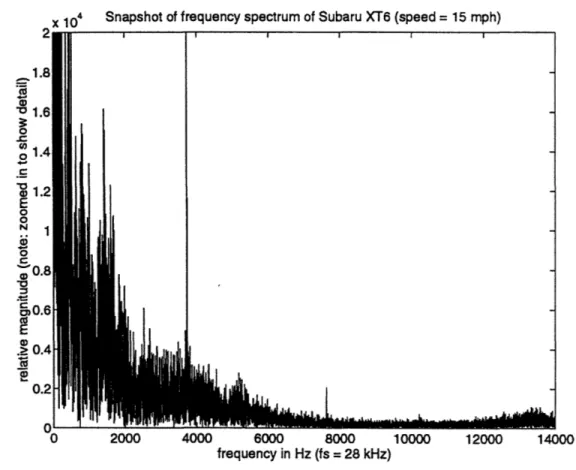
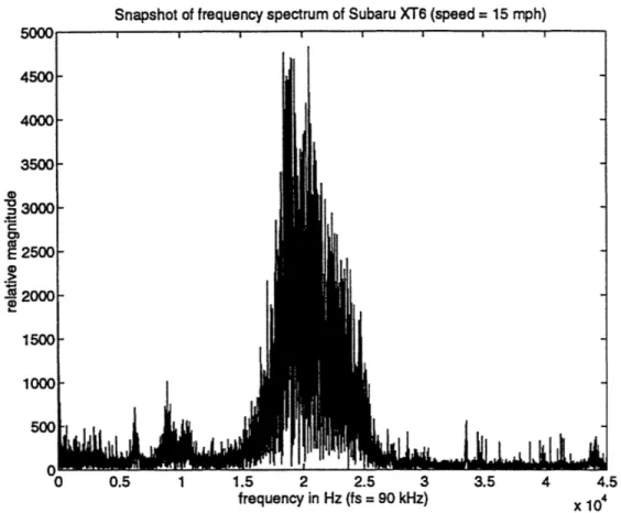
In the spectra for both vehicles, signal power is dominant for frequencies up to 8 kHz as seen in Figure 3-6. However, in the band between 8-15 kHz, noise seems to be the major contributor. Surprisingly, examination of the outputs of the ultrasonic microphones, reveals significant signal power in the range from 15-27 kHz (refer to Figure 3-7. It is uncertain whether there is signal power at frequencies greater than 27 kHz because the frequency response of the ultrasonic microphones begins to roll off at

Parabolic

Reflector

0=

microphone

Figure 3-4: Microphone mounting boxes

26 kHz and the analog recorder rolls off at 20 kHz.2 _{Originally, it was hypothesized}

that this energy was due to the wind generated by the moving vehicle. However, it was later discovered during Field Test Two that most of the energy at the high end of the spectrum is likely due to tire/road interface noise.

Closer examination of the regions where signal power is dominant does not reveal obvious peaks which can be tracked. This is probably due to the large number of

distributed acoustic sources in a vehicle, such as the engine in the front and the

muffler in the back. Furthermore, if a vehicle proceeds rapidly through the spatial detection zone (especially in the nearest lane), the associated Doppler shift can be large and difficult to track. The difficulty of tracking wideband Doppler shifts led to consideration of alternate processing techniques such as wavelets, short-term Fourier

2

Signal power up to 27 kHz appears significant enough to be detectable even though the equipment bandwidth is less than 27 kHz.

(+z direction is skyward;

i.e. out of the page)

---... ->+x

Svehicle

NOTE: Drawing not to scale;

Aerial view of alley

(air hoses)

Figure 3-5: Accelerometer measurement axes for Field Test One transforms, and time correlation.

The speed estimation algorithm which focuses upon tracking the change in time delay between a pair of microphones (refer to Section 4.4) was applied to the data set. The delay in signal arrival time between two spatially separated microphones will be denoted by T. In Field Test One, the vertical range component (Ry) was known and a three-element array was unnecessary. The shapes of the 7 vs. time curves obtained from correlating the outputs of the Radio Shack microphones were exactly as expected, which was promising. There is a tradeoff between using longer correlation windows, which yield smoother curves but are more likely to violate the assumption of quasi-stationarity, and shorter windows, which yield noisier but more accurate curves. For the sampling rate of 35 kHz, using 1000 point correlation windows (overlapped by 500 points) to measure 7 returned fairly accurate speed estimates when the 7 vs. time plot was fitted with a fifth-order polynomial.

A curve generated using a 1000 sample correlation window (for

f,

= 35 kHz) with 50% overlap between windows is shown in Figure 3-8. It corresponds to an experiment where the Subaru XT6 was driven by at a constant speed of 14.53 mph (according

x 104 Snapshot of frequency spectrum of Subaru XT6 (speed = 15 mph) " 1 4, -01 o "0 01 E 0 0 N o 0 (o E .> 0 o frequency in Hz (fs = 28 kHz)

Figure 3-6: Spectrum of the Subaru XT6 as measured by a Radio Shack microphone (snapshot)

to the verification system). Since RY was very short during Field Test One, two -r

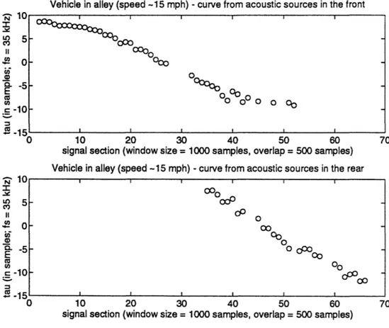
vs. time curves were distinguishable. These were attributed to acoustic sources in the front (such as the engine and front wheels) and rear (such as the muffler and rear wheels) of the vehicle. After discarding noisy values, a fifth-order polynomial curve-fit yielded speed estimates of 11.27 mph for the front acoustic sources and 14.00 mph for the rear. The separated curves for each set of acoustic sources (augmented with

T estimates from the second and third largest peaks) appear in Figure 3-9.

These speed estimates should be taken as an indication of algorithm potential rather than precision. In retrospect, there were several factors which could have degraded the r estimates (f): aliasing, machinery noise, echoes, the omnidirectional microphones, and the nearness of the sensors to the source. Anti-aliasing filters were not included in the analysis sequence until road test data was analyzed. Consequently,

Snapshot of frequency spectrum of Subaru XT6 (speed = 15 mph)

~I I I

I ii

0.5 1 1.5 2 2.5 3

frequency in Hz (fs = 90 kHz) 3.5 4 _{x 10}4.5

Figure 3-7: Spectrum of the Subaru XT6 as measured (snapshot)

by an ultrasonic microphone

in the sampled data from Field Tests One and Two3, frequencies above 17.5 kHz were aliased down to baseband. As noted earlier, there is a considerable amount of high frequency energy from 17-27 kHz due to tire/road interface noise. Quite possibly, the Radio Shack microphones detected the high frequency contributions, especially since the sensors were situated so close to the lane. To investigate this theory, data from the above experiment was resampled using anti-aliasing filters. The new T vs. time plot from the filtered data was similar to the original obtained from the unfiltered data. Furthermore, the spectra from both sets of data were nearly identical. Hence, it seems safe to assume that the frequency response of the Radio Shack microphones falls off well below 17 kHz. The remainder of the Radio Shack microphone data from Field Tests One and Two was not resampled.

3_{Field Test Three was conducted}

after Road Test Two.

bUUU 4500 4000 3500 3000 C: E 2500 2000 1500 1000 500 I I I

ýI

I .I

kil a

I I I I

I-Vehicle in alley (speed = -15 mph, Ry = 8 ft, array spacing = 8 in) 10 N II5 0 E -( ca -10

I r

0 20 40 60 80 100 120 140 160 signal section (window size = 1000 samples, overlap = 500 samples)

Figure 3-8: T vs. time for the Subaru XT6

(using only dominant peaks)

There appeared to be a strong low frequency component in the audible range data (at 40 Hz for the car and at 50 Hz for the pickup truck). At the time, it was uncertain whether the "spike" was due to signal or noise power since the frequency response of the microphones was unknown. Nonetheless, in retrospect, it appears that it could be a signal component since its magnitude increases as the vehicle approaches and decreases as it departs. The peak did not appear to shift in frequency while the vehicle was in the detection zone which suggested that it might be noise. However, for low frequencies, the Doppler effect (which is a function of frequency) is very small and would not be detectable with the given frequency resolution. Currently, it is suspected that it is a signal component which warrants further consideration.4 Determination

4_{For the construction vehicle from Field Test Two, a spike appeared at 80 Hz.}

0 o o 0 0 0 00

0

o0

00

oo

oo

00 I I I I I I 0•

I

Vehicle in alley (speed -15 mph) - curve from acoustic sources in the front -" 0 0000 N oo c .-5 - 0o O0o II _{o o o} Ca 010 0 _{o0%o 0 0} " -10 OI I 0 10 20 30 40 50 60 70

signal section (window size = 1000 samples, overlap = 500 samples) Vehicle in alley (speed -15 mph) - curve from acoustic sources in the rear

0000 N0 - 0 5" -5 o ooo :C U, 00 C -10 - ₄ 00 * I 1 5 0 10 20 30 40 50 60 70

signal section (window size = 1000 samples, overlap = 500 samples)

Figure 3-9: Separated curves for acoustic sources in front and rear of Subaru XT6

(after addition of supplemental points)

of whether the spike is definitely due to signal or noise is left for the future.5

The large mean squared-errors (MSE) in some of the -f from this data set probably resulted from the close proximity of the sensors to the source and from echoes in the alley. As the vehicle/sensor separation is narrowed, the time interval over which the assumption of quasi-stationarity is valid becomes shorter. Furthermore, the omnidi-rectional nature of the microphones allowed them to detect sounds from behind the array, which included machinery noise and echoes from the wall directly behind the microphones.

With regard to the ultrasonic data (sampled at 45 ksps), the time delay estimates

5_{During the road tests, a two-pole highpass filter with a cutoff frequency of 80 Hz was included}

which effectively rejected this frequency component along with other noise. The highpass filter was included because the frequency response of the Sennheiser microphones used in the road tests was limited at the low end to 50 Hz.

were much worse. This could have arisen from several factors. First, since there was no anti-aliasing filter applied, frequency components above 22.5 kHz were aliased into the baseband. Furthermore, because the frequencies of interest are high relative to the sampling rate, the number of samples/cycle for a given frequency is very low (3 or less). Thus, inaccuracies from discrete correlation should be expected. Theoretically, if the sampling rate was increased so that the number of samples/cycle was much larger, the f- should improve. The same effect is achieved by bandpass filtering the data from 15-30 kHz then sampling at 30 ksps. In this way, the frequencies from 15-30 kHz will be shifted down to baseband (0-15 kHz) which effectively raises the number of samples/cycle. The algorithm is applied to the bandshifted signal to yield better delay estimates. This idea and others are presently under investigation.

The accelerometers seemed to detect very little motion from the vehicles. Since it is more likely that an accelerometer would sense vertical motion rather than lateral motion when a vehicle passes, a triax seemed unnecessary. Hence when the traffic on Hartwell Avenue was measured, only one accelerometer sensing translational motion was placed on the road.

Strangely enough, the PCB accelerometers pointed in the y and z directions were able to detect a vehicle's horn very faintly. It is suspected that the accelerometers were detecting air vibration rather than ground vibration. This sparked interest in the possible use of accelerometers for measuring low frequency air vibration since the Sennheiser microphones are not very sensitive to frequencies below 50 Hz. The ADXL50 sensor on a flexible membrane during Road Test One was a crude attempt to realize such a low frequency microphone.

Finally, it was noted that the radar dishes did not seem to offer much improve-ment for the Radio Shack microphones. They provided only a slight gain increase. Nonetheless, it is possible that they would improve the performance of the ultrasonic sensors. The focusing effect of the dish might provide enough gain to noticeably in-crease their limited detection range. However, because of the short wavelengths of the frequencies involved, reflections would likely introduce random phase shifts which would make time delay estimation difficult.

3.2.2

Field Test Two

The second field test was conducted on a side street that runs perpendicular to the alley used in the first field test. This wide, open site was chosen for several reasons: to avoid echo problems, to allow more distance between the sensors and the source (for larger RP), and to provide enough space for vehicles to be driven by at different distances. The main objectives of this test were to roughly estimate the range capa-bilities of the microphones, measure a sample vehicle's "resting" spectrum by letting it idle by the microphones, and examine signals from possible noise sources.

Since only microphones were considered in this test, the structure in the diagram of Figure 3-10 was nailed to the pavement. Both audible range (Radio Shack) and ultrasonic microphones were included because the final sensor design might involve a hybrid of both. The two microphone mounting boxes from Field Test One (from Figure 3-4) were attached with tie wraps to a hollow aluminum pole for support. The pole was connected to an optical mount which was attached to the pavement with nails. The ultrasonic microphones, which are more sensitive to tire/road interface noise, were positioned closer to the ground at a height of 16 inches. However, they were not placed too near the ground to avoid multipath problems from signals bounc-ing off the pavement. The Radio Shack microphones were placed at a height of 26 inches.

While viewing the outputs of the ultrasonic microphones with an oscilloscope, their extreme sensitivity to abrasive noise was discovered when a pedestrian walked by. As an indication of their sensitivity, they were able to detect a person scraping his feet on the ground 20 feet away. Since sensitivity to pedestrians would introduce noise to the measurements, several instances of a person walking by from various positions were recorded for future reference.

With the audible range microphones, a person can easily be distinguished from a car since their spectral characteristics are different. For the person walking, the detected signal is primarily due to interface noise. Examining short-term Fourier transforms (STFTs) of windowed sections reveals that the spectral shape and magni-tude stay fairly constant. In contrast, due to the large number of distributed acoustic

0=

Radio Shack microphone

0=

ultrasonic microphone

NOTE: Drawing not to scale

Figure 3-10: Microphone assembly for Field Test Two

sources on a vehicle, its spectral shape varies and its magnitude tends to increase as the vehicle is approaching and decrease as it departs. As the vehicle departs, however, the STFT plots tend to assume a shape similar to that of a person walking.

Data from airplanes flying overhead was also collected. The ultrasonic micro-phones were not sensitive their presence. This is explained by the fact that in the air, higher frequencies are attenuated faster than low frequencies. The Radio Shack mi-crophones did detect the planes, which poses a potential problem for vehicle tracking. At worst, there might be a few missed detections while a plane is overhead. However, since vehicles will be much closer than the airplane, they should be the dominant sources and the delay estimates will likely reflect their motion more than the plane's motion. The effect of plane noise can be reduced by replacing each microphone in the array with a cluster of microphones and using beamforming techniques to generate

a narrow-beam "acoustic center". Improved T estimates are obtained by examining the delays between the effective acoustic centers.

Another objective of Field Test Two was to get an idea of the spectrum of various engine components. A few trials were run with a sample vehicle (the Toyota pickup truck) idling directly next to the microphones in a few different positions. Data was collected with the vehicle directly facing the microphone array (head on) and with the left front wheel directly next to the array. In retrospect, since people drive on the right side of the road in the United States it would have been better to place the

vehicle's right front wheel next to the array. However, this can easily be done later if it becomes necessary. Though the current vehicle tracking algorithm does not depend on the contents of the vehicle's acoustic spectrum, the data was obtained for future reference. In Field Test Three, a vehicle (the Subaru XT6) with its tailpipe next to

the array was recorded.

In another series of tests, sensor range capabilities were studied while the Toyota truck was driven by at distances of approximately 10, 20, and 30 feet. The Radio Shack microphones performed well; the speed estimates obtained from correlating their outputs appeared reasonable. However, they were not be verified because vehicle speed was not recorded (since only range effects were investigated in this field test). The ultrasonic microphones also proved capable of detecting the vehicle 30 feet away. This is promising since it is desirable for the passive acoustic sensor to be able to monitor multiple-lane roads which may have lane widths of 8 feet or more. Range capabilities might be extended with further amplification or focusing, but this has not been determined.

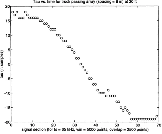
A typical 7 vs. time curve obtained from correlating two Radio Shack microphones is shown in Figure 3-11. This curve was generated using a correlation window of 5000 points with an overlap of 2500 points with a sampling rate of 35 kHz. It was obtained from an experiment where the Toyota truck was driven by the array at a distance of 30 feet. A speed estimate of 13.5 mph was returned, which appears reasonable. It was noted that the 7 vs. time curves in general were much smoother than those obtained from Field Test One due to the increased source/array distances (which increased

stationarity over the correlation windows). Furthermore, due to the increased Ry the vehicle remained in the detection zone for a longer period of time, generating more points for the T vs. time curve (for more accurate curve-fitting) and allowing use of longer correlation windows if desired.

Tau vs. time for truck passing array (spacing = 8 in) at 30 ft

10 20 30 40 50 60

signal section (for fs = 35 kHz, win = 5000 points, overlap = 2500 points)

Figure 3-11: 7 vs. time plot for pickup truck passing array at 30 ft

Since a Honda EX1000 generator would be providing power for the upcoming road tests, there was some concern whether its presence would contribute significant background noise. When the array outputs were examined with an oscilloscope, it appeared that the generator raised the background noise levels of both sets of microphones, though the ultrasonic only slightly. Standing in front of the generator seemed to block most of the acoustic power, so for the road tests, sound deadening material was placed in front of it. The generator was not used in Field Tests One or Two.

One final important observation from Field Test Two was made when a

construc-000 construc-00000 0 00 00 0 000 00OO_CO 0 O0 O0 0 O O 00₀₀ O 00 0 O 0O0 000 O 000 00 00 00 O 0 ₀ 000000000000

20

0

-tion vehicle drove past the array in the opposite direc-tion that the truck had been traveling. Its crossing was recorded (the truck was not in the field) and the correlation technique applied. In comparing the T vs. time curves of the construction vehicle and the truck, they had similar shapes as expected. However, their slopes were of

oppo-site sign, indicating they had been traveling in oppooppo-site directions! This observation

agreed well with theory and strongly supported the notion that bidirectional traffic could be monitored with a single sensor. It also demonstrated that determining a vehicle's direction of travel would be trivial. Cases involving bidirectional traffic were examined using data from the road tests.

Upon completion of Field Test Two, the stage was set for analyzing real traffic data. A preliminary algorithm had been developed which involved correlating the outputs of a pair of microphones over short observation intervals to obtain time delay estimates (f). After plotting the -? vs. time, it was shown experimentally that the speed of the vehicle is proportional to the slope at the inflection point, as expected from theory. When the range of the vehicle is known, the algorithm yields an accurate speed estimate. However, a reliable means for determining range must be formulated. Methods involving triangulation using a colinear three-sensor array are nonlinear and highly sensitive to noisy time delay estimates. Extended Kalman filtering (EKF) techniques, which compensate for noisy measurements, are suggested for improving the range and bearing estimates from triangulation. Alternatively, a lesser-known algorithm pinpoints the source's location on a conic axis (LOCA) using time delay estimates from an array of three noncolinear sensors. Even though LOCA is also sensitive to noisy 'I, it yields more promising range estimates than triangulation. These three range finding techniques are discussed in greater detail in Section 4.5.

3.2.3

Field Test Three

In order to observe the contribution of tire/road interface noise to the ultrasonic spectrum, a vehicle was allowed to "coast" past the microphone array in neutral with the engine off during Field Test Three. The sensors for the experiment were the lower three-element microphone arrays (Sennheiser audible range and ultrasonic) from Road

Test Two (refer to Figure 3-16). The arrays were located approximately three feet from the road. Since the engine was off, the microphones' outputs primarily reflected tire/road interface noise. Examination of the output of one of the ultrasonic sensors revealed a signal that had the same general characteristics (bandwidth, bandshape, amplitude, time envelope shape) as those seen in other tests where the engine was on. During Field Test Two, the spectra of idling vehicles (which predominantly reflected engine noise) which were positioned directly next to the ultrasonic microphones also exhibited ultrasonic energy. However, it is suspected that when vehicles are more distant, the contribution of engine noise to the ultrasonic spectrum will be much smaller.

Viewing the contribution of the tire/road interface noise in the audible spectrum suggested an interesting avenue to pursue in the future. Examination of STFTs of overlapping short segments of the audible range data revealed a spectrum whose magnitude increased then decreased as the vehicle coasted by as expected. The bandwidth was approximately 8 kHz. Despite the dynamics of the spectrum as the vehicle passed, the frequencies in the band from 6 to 8 kHz remained distinct from the rest of the spectrum (see Figure 3-12). When STFTs of data from the road tests were analyzed for comparison, the spectra exhibited the same dynamic property of increasing as the vehicle approached and decreasing as it departed. However, as a vehicle neared the array, the power in the range from approximately 5 to 8 kHz (depending on the vehicle type) would suddenly increase then decrease as the vehicle moved out of range. Presumably, these power "bursts" were shorter in duration than the one observed in Field Test Three because the vehicles on the road were farther away and traveling more rapidly. The power burst provides an indication that a vehicle is approaching the array and is near the "inflection" point (which is the point where the vehicle is directly in front of the array). It is thought that these bursts are due to audible range tire/road interface noise. If this is the case, it might be worthwhile to try frequency domain processing techniques to see if an alternative method to measure speed can be found by focusing on this band. If speed can be determined in this manner, then employing the correlation technique would provide

lane information (R,) and direction of travel. 1-UUU 1000( 800( 600( 400( 200(

Snapshot of frequency spectrum of vehicle coasting by in neutral

,1il

11"11

,'* .

I.

-Ir.I,,1 J

4000 6000 8000

frequency in Hz (fs = 28 kHz)

10000 12000 14000

Figure 3-12: Spectrum of vehicle coasting by in neutral (snapshot)

The car coasting by in neutral was easily tracked by the audible range microphones using the correlation technique. This suggests that in the future, tracking "quiet" vehicles with audible range microphones should not pose a problem. On the other hand, a problem arose when the 7 vs. time plot was viewed. Two essentially parallel curves were evident, one for each axle, as seen in Figure 3-13. Apparently, because of the nearness of the array, the axles were separated enough that each set was tracked independently. Hence, trucks and other long vehicles with widely separated axles might be miscounted as two vehicles if they pass too closely to the array. This could be avoided by increasing the distance from the array to the road (Yo), but this might hurt the performance of the correlation algorithm since SNR is lower and estimate biases will amplify as range is increased. Furthermore, increasing the distance would not be practical for the short-range ultrasonic microphones. A better approach would be to

2000 I II i..

di

' -F F

I

I