Climate dynamics and fluid mechanics: Natural variability and related uncertainties

HAL Id: hal-00184946

https://hal.archives-ouvertes.fr/hal-00184946

Preprint submitted on 4 Nov 2007

HAL is a multi-disciplinary open access

archive for the deposit and dissemination of

sci-entific research documents, whether they are

pub-lished or not. The documents may come from

teaching and research institutions in France or

L’archive ouverte pluridisciplinaire HAL, est

destinée au dépôt et à la diffusion de documents

scientifiques de niveau recherche, publiés ou non,

émanant des établissements d’enseignement et de

recherche français ou étrangers, des laboratoires

Climate dynamics and fluid mechanics: Natural

variability and related uncertainties

Michael Ghil, Mickael D. Chekroun, Eric Simonnet

To cite this version:

Michael Ghil, Mickael D. Chekroun, Eric Simonnet. Climate dynamics and fluid mechanics: Natural

variability and related uncertainties. 2007. �hal-00184946�

Climate dynamics and fluid mechanics:

Natural variability and related uncertainties

Michael Ghil

D´epartement Terre-Atmosph`ere-Oc´ean, Laboratoire de M´et´eorologie Dynamique (CNRS and IPSL) and

Environmental Research and Teaching Institute, ´

Ecole Normale Sup´erieure, 75231 Paris Cedex 05, France;

Department of Atmospheric Sciences and Institute of Geophysics and Planetary Physics, University of California, Los Angeles, CA 90095-1565, USA

Mickael D. Chekroun¨

Environmental Research and Teaching Institute, ´

Ecole Normale Sup´erieure, 75231 Paris Cedex 05, France

Eric Simonnet

Institut Non Lin´eaire de Nice (INLN)-UNSA, UMR 6618 CNRS,

1361, route des Lucioles 06560 Valbonne - France

Abstract

The purpose of this review-and-research paper is twofold: (i) to review the role played in climate dynamics by fluid-dynamical models; and (ii) to contribute to the understanding and reduction of the uncertainties in future climate-change projections. To illustrate the first point, we review recent theoretical advances in studying the driven circulation of the oceans. In doing so, we concentrate on the large-scale, wind-driven flow of the mid-latitude oceans, which is dominated by the presence of a larger, anticyclonic and a smaller, cyclonic gyre. The two gyres share the eastward extension of western boundary currents, such as the Gulf Stream or Kuroshio, and are induced by the shear in the winds that cross the respective ocean basins. The boundary currents and eastward jets carry substantial amounts of heat and momentum, and thus contribute in a crucial way to Earth’s climate, and to changes therein.

Changes in this double-gyre circulation occur from year to year and decade to decade. We study this low-frequency variability of the wind-driven, double-gyre circulation in mid-latitude ocean basins, via the bifurcation sequence that leads from steady states through periodic solutions and on to the chaotic, irregular flows documented in the observations. This sequence involves local, pitchfork and Hopf bifurcations, as well as global, homoclinic ones.

The natural climate variability induced by the low-frequency variability of the ocean circulation is but one of the causes of uncertainties in climate projections. The range of these uncertainties has barely decreased, or even increased, over the last three decades. Another major cause of such uncertainties could reside in the structural instability—in the classical, topological sense—of the equations governing climate dynamics, including but not restricted to those of atmospheric and ocean dynamics.

We propose a novel approach to understand, and possibly reduce, these uncertain-ties, based on the concepts and methods of random dynamical systems theory. The idea is to compare the climate simulations of distinct general circulation models (GCMs) used in climate projections, by applying stochastic-conjugacy methods and thus perform a stochastic classification of GCM families. This approach is particularly appropriate given recent interest in stochastic parametrization of subgrid-scale processes in GCMs. As a very first step in this direction, we study the behavior of the Arnol’d family of circle maps in the presence of noise. The maps’ fine-grained resonant landscape is smoothed by the noise, thus permitting their coarse-grained classification.

Key words: Climate change, physical oceanography, dynamical systems, bifurcations, structural stochastic stability, Arnol’d tongues.

1

Introduction and motivation

Charney et al. [1] carried out the first attempt to obtain a consensus estimate of the equi-librium sensitivity of climate to changes in atmospheric CO2 concentrations. The result was

the now famous range of 1.5 K to 4.5 K for a doubling of this concentration.

As the relatively new science of climate dynamics evolved through the 1980s and 1990s, it became quite clear — from observational data, both instrumental and paleoclimatic, as well as model studies — that Earth’s climate never was and is unlikely to ever be in equilibrium. The three successive IPCC reports (1991 [2], 1996, and 2001 [3]) concentrated therefore, in addition to estimates of equilibrium sensitivity, on estimates of climate change over the 21st century, based on several scenarios of CO2 increase over this time interval, and using up to

18 general circulation models (GCMs) in the fourth IPCC Assessment Report (AR4) [4]. The GCM results of temperature increase over the coming 100 years have stubbornly resisted any narrowing of the range of estimates, with results for Tsin 2100 as low as 1.4 K

or as high as 5.8 K, according to the Third Assessment Report. The hope in the research leading up to the AR4 was that a set of suitably defined “better GCMs” would exhibit a narrower range of year-2100 estimates, but this does not seem to have been the case.

Figure 1: Frequency distributions of global mean, annual mean, near-surface temperature (Tg) for 2,017 GCM simulations, and doubled CO2 (from [7]).

The difficulty in narrowing the range of estimates for either equilibrium sensitivity of climate or for end-of-the-century temperatures is clearly connected to the complexity of the climate system, the multiplicity and nonlinearity of the processes and feedbacks it contains, and the obstacles to a faithful representation of these processes and feedbacks in GCMs. The practice of the science and engineering of GCMs over several decades has amply demonstrated

that any addition or change in the model’s “parametrizations” — i.e., of the representation of subgrid-scale processes in terms of the model’s explicit, large-scale variables — may result in noticeable changes in the model solutions’ behavior.

As an illustration, Fig. 1 shows the sensitivity of an atmospheric GCM, which does not include a dynamical ocean, to changes in its model parameters. Several thousand simulations were performed as part of the “climateprediction.net” experiment [5], using perturbations in several parameters of the Hadley Centre’s HadAM3 model [6], coupled to a passive, mixed-layer ocean model. The figure clearly illustrates a wide range of responses to CO2doubling,

from 2 K to more than 11 K [7].

The last IPCC report [4] has investigated climate change as a result of various scenarios of CO2increase as well, for a set of 18 distinct GCMs. The best estimate of the temperature

change at the end of the 21st century from AR4 is about 4.0◦ _{C for the worst scenario of}

greenhouse-gas increase, namely A1F1, roughly speaking a future world with a very rapid economic growth. The likely range of end-of-century global temperatures is of 2.4-6.4◦ _{C in}

this case, and comparably large ranges of uncertainties obtain for all other scenarios as well [4].

An essential contributor to this range of uncertainty is natural climate variability [8] of the coupled ocean-atmosphere system. As mentioned already in [9], most GCM simula-tions do not exhibit the observed interdecadal variability of the oceans’ buoyancy-driven, thermohaline circulation [10]. Another striking example of low-frequency, interannual-and-interdecadal variability is provided by the near-surface, wind-driven ocean circulation [10, 11]. The influence of strong thermal fronts — like the Gulf Stream in the North Atlantic or the Kuroshio in the North Pacific — on the mid-latitude atmosphere above is severely underes-timated. Typical spatial resolutions in the century-scale GCM simulations of [2, 3, 4, 5, 6, 7] are of the order of 100 km at best, whereas resolutions of 20 km and less would be needed to really capture the strong mid-latitude ocean-atmosphere coupling just above the oceanic fronts [12, 13].

The purpose of this paper is twofold. First, we describe in Section 2 the most recent theoretical results regarding the internal variability of the mid-latitude wind-driven circula-tion, viewed as a problem in nonlinear fluid mechanics. These results rely to a large extent on the deterministic theory of dynamical systems [14, 15]. Second, we address in Section 3 the more general issue of uncertainties in climate change projections. Here we rely on concepts and methods from random dynamical systems theory [16] to help understand and possibly reduce these uncertainties. Much of the material in the latter section is new, and it is supplemented by some rigorous mathematical results in Appendix A. A summary and an outlook on future work follow in Section 4.

2

Natural variability of the wind-driven ocean

circula-tion

2.1

Observations

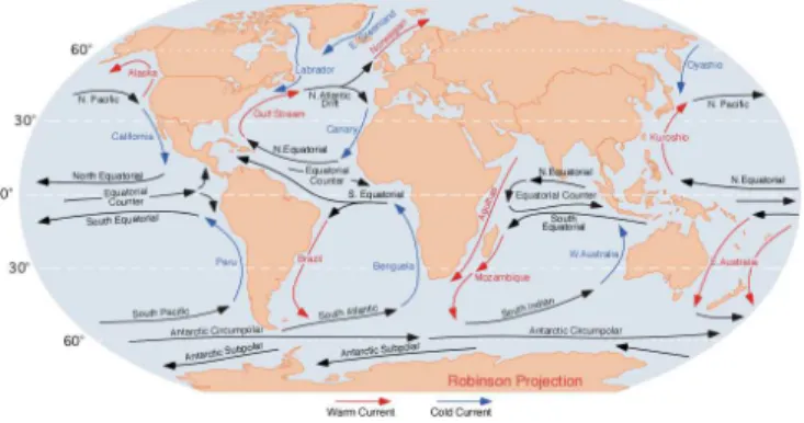
To a first approximation, the main oceanic currents are driven by the mean effect of the winds. The trade winds near the equator blow mainly from east to west and are called also the tropical easterlies. In mid-latitudes, the dominant winds are the prevailing westerlies, and towards the poles the winds are easterly again. Three of the strongest near-surface, mid-and-high-latitude currents are the Antarctic Circumpolar Current, the Gulf Stream in the North Atlantic, and the Kuroshio Extension east off Japan. The Antarctic Circumpolar

Current, sometimes called the Westwind Drift, circles eastward around Antarctica; see Fig. 2.

Figure 2: A map of the main oceanic currents: warm currents in red and cold ones in blue. The Gulf Stream is an oceanic jet with a strong influence on the climate of eastern North America and of western Europe. Actually, the Gulf Stream is part of a larger, gyre-like current system, which includes the North Atlantic Drift, the Canary Current and the North Equatorial Current. It is also coupled with the slow pole-to-pole thermohaline or overturning circulation, with cold denser water masses sinking in the subpolar North Atlantic and lighter water rising over much wider areas of the low and southern latitudes. From Mexico’s Yucatan Peninsula, the Gulf Stream flows north through the Florida Straits and along the East Coast of the United States. Near Cape Hatteras, it detaches from the coast and begins to drift off into the North Atlantic towards the Grand Banks near Newfoundland.

The Coriolis force is responsible for the so-called Ekman transport, which deflects water masses orthogonally to the near-surface wind direction and to the right [17, 18, 19]. In the North Atlantic, this Ekman transport creates a divergence and a convergence of near-surface water masses, respectively, resulting in the formation of two oceanic gyres: a smaller, cyclonic one in subpolar latitudes, the other larger and anticyclonic in the subtropics. This type of double-gyre circulation characterizes all mid-latitude ocean basins, including the South Atlantic, as well as the North and South Pacific.

The double-gyre circulation is intensified as the currents approach the East Coast of North America due to the β-effect. This effect is mainly due to the variation of the Coriolis force with latitude, while the oceans’ bottom topography also contributes to it. The former, planetary β-effect is of crucial importance in geophysical flows and induces free Rossby waves propagating westward [17, 18, 19].

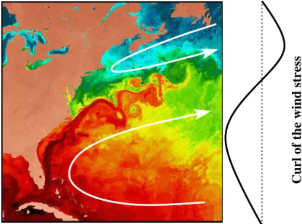
The currents along the western shores of the North Atlantic and of the other mid-latitude ocean basins exhibit boundary-layer characteristics and are commonly called western boundary currents (WBCs). The northward-flowing Gulf Stream and the southward-flowing Labrador Current extension meet near Cape Hatteras and yield a strong eastward jet. The formation of this jet and of the intense recirculation vortices near the western boundary, to either side of the jet, is mostly driven by internal, nonlinear effects. Figure 3 illustrates how these large-scale wind-driven oceanic flows self-organize, as well as the resulting eastward jet. Different spatial and time scales contribute to this self-organization, mesoscales eddies playing the role of the synoptic-scale systems in the atmosphere. Warm and cold rings last for several months up to a year and have a size of about 100 km; two cold rings are clearly visible in Fig. 3. Meanders involve larger spatial scales, up to 1000 km, and are associated with interannual variability. The characteristic scale of the jet and gyres is of several

thou-sand kilometers and they exhibit their own intrinsic dynamics on time scales of several years to possibly several decades.

A striking feature of the wind-driven circulation is the existence of two well-known North-Atlantic oscillations, with a period of about 7 and 14 years, respectively. Data analysis of various climatic variables, such as sea surface temperature (SST) over the North Atlantic or sea level pressure (SLP) over western Europe [20, 21] and local surface air temperatures in Central England [22], as well as of proxy records, such as tree rings in Britain, travertine concretions in southeastern France [23], and Nile floods over the last millennium or so [24], all exhibit strikingly robust oscillatory behavior with a 7-yr period and, to a lesser extent, with a 14-yr period. Variations in the path and intensity of the Gulf Stream are most likely to exert a major influence on the climate in this part of the world [25]. This is why theoretical studies of the low-frequency variability of the double-gyre circulation are important.

Given the complexity of the processes involved, climate studies have been most successful when using not just a single model but a full hierarchy of models, from the simplest “toy” models to the most detailed GCMs [26]. In the following, we describe one of the simplest models of the hierarchy used in studying this problem.

Curl of the wind stress

Figure 3: A satellite image of the sea surface temperature (SST) over the northwestern North Atlantic, together with a sketch of the associated double-gyre circulation. An idealized view of the amount of potential vorticity injected into the ocean circulation by the trade winds, westerlies and polar easterlies is shown to the right.

2.2

A simple model of the double-gyre circulation

The simplest model that includes many of the mechanisms described above is governed by the barotropic quasi-geostrophic (QG) equations. The term geostrophic refers to the fact that large-scale rotating flows tend to run parallel to, rather than perpendicular to constant-pressure contours; in the oceans, these contours are associated with the deviation from rest of the surfaces of equal water mass, due to Ekman pumping. Geostrophic balance implies in particular that the flow is divergence-free. The term barotropic, as opposed to baroclinic, has a slightly different meaning in geophysical fluid dynamics (GFD) than in engineering fluid mechanics: it means that the model describes a single fluid layer of constant density and therefore the solutions do not depend on depth [17, 18, 19].

We consider an idealized, rectangular basin geometry and simplified forcing that mimics the distribution of vorticity contribution by the winds, as sketched to the right of Fig. 3.

In our idealized model, the amounts of subpolar and subtropical vorticity injected into the basin are equal and the rectangular domain Ω = (0, Lx) × (0, Ly) is symmetric about the

axis of zero wind stress curl. The barotropic two-dimensional (2-D) QG equations in this idealized setting are:

qt+ J(ψ, q) − ν∆2ψ + µ∆ψ = −τ sin2πy_L y ,

q = ∆ψ − λ−2_R ψ + βy. (2.1)

Here q and ψ are the potential vorticity and streamfunction, respectively, and the Jacobian J corresponds to the advection of potential vorticity by the flow, J(ψ, q) = ψxqy−ψyqx= u·∇q,

where u = (−ψy, ψx), x points east and y points north. The physical parameters are the

strength of the planetary vorticity gradient β, the Rossby radius of deformation λ−2_R , the eddy-viscosity coefficient ν, the bottom friction coefficient µ, and the wind-stress intensity τ . We use here free-slip boundary conditions ψ = ∆2_{ψ = 0; the qualitative results described}

below do not depend on the particular choice of homogeneous boundary conditions. We consider (2.1) as an infinite-dimensional dynamical system and study its bifurcation sets as the parameters change. Two key parameters are the wind stress intensity τ and the eddy viscosity ν. An important property of (2.1) is its mirror symmetry in the y = Ly/2

axis. This symmetry can be expressed as invariance with respect to the discrete Z2group S:

S [ψ(x, y)] = −ψ(x, Ly− y); (2.2)

any solution of (2.1) is thus accompanied by its mirror-conjugated solution. Hence, in generic terms, the prevailing bifurcations are of either the symmetry-breaking or the saddle-node or the Hopf type.

2.3

Bifurcations in the double-gyre problem

The historical development of a comprehensive nonlinear theory of the double-gyre circula-tion is interesting on its own, having seen substantial progress in the last 15 years. One can distinguish four main steps.

2.3.1 Symmetry-breaking bifurcations

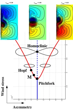
The first step was to realize that the first generic bifurcation of this QG model was a genuine pitchfork bifurcation that breaks the system’s symmetry as the nonlinearity becomes large enough [27, 28, 29]. The situation is shown in Fig. 4. When the forcing is weak or the dissipation is large, there is only one steady solution, which is antisymmetric with respect to the mid-axis of the basin. This solution exhibits two large gyres, along with their typical, β-induced WBCs. Away from the western boundary, such a near-linear solution (not shown) is dominated by Sverdrup balance between wind stress curl and the meridional mass transport [17, 30].

As the wind stress increases, the near-linear Sverdrup solution develops an eastward jet along the mid-axis, which penetrates farther into the domain. This more intense, and hence more nonlinear solution is still antisymmetric about the mid-axis, but loses its stability for some critical value of the wind-stress intensity (indicated by “Pitchfork” in Fig. 4). A pair of mirror-symmetric solutions emerges and is characterized by a rather different vorticity distribution; the streamfunction fields associated with the two stable steady-state branches are plotted to the upper-left and right of Fig. 4. In particular, the jet in such a solution exhibits a large meander, reminiscent of the one seen in Fig. 3 just downstream of Cape Hatteras; note that the colors in Fig. 4 have been chosen to facilitate the comparison with

2.5 3 3.5 4 x 10 −4 −8 −6 −4 −2 0 2 4 6 x 10 −4 wind−stress intensity || subtropical − subpolar || 2 rH = 374 m 2 s −1 , grid = 15 km ✁ ✁ ✁ ✁ ✁ ✁ ✂ ✂ ✂ ✂ ✂ ✂ ✄ ✄ ✄ ✄ ✄ ✄ ☎ ☎ ☎ ☎ ☎ ☎ ✆ ✆ ✆ ✆ ✆ ✆ ✝ ✝ ✝ ✝ ✝ ✝ ✞ ✞ ✞ ✟ ✟ ✟ ✟ ✟ ✟ ✟ ✟ ✟ ✟ ✟ ✟ ✟ ✟ ✟ ✟ ✟ ✟ ✟ ✟ ✟ ✟ ✟ ✟ ✟ ✟ ✟ ✟ ✟ ✟ ✟ ✟ ✟ ✟ ✟ ✟ ✟ ✟ ✟ ✟ ✟ ✟ ✟ ✟ ✟ ✟ ✟ ✟ ✟ ✟ ✟ ✟ ✟ ✟ ✟ ✟ ✟ ✟ ✠ ✠ ✠ ✠ ✠ ✠ ✠ ✠ ✠ ✠ ✠ ✠ ✠ ✠ ✠ ✠ ✠ ✠ ✠ ✠ ✠ ✠ ✠ ✠ ✠ ✠ ✠ ✠ ✠ ✠ ✠ ✠ ✠ ✠ ✠ ✠ ✠ ✠ ✠ ✠ ✠ ✠ ✠ ✠ ✠ ✠ ✠ ✠ ✠ ✠ ✠ ✠ ✠ ✠ ✠ ✠ ✠ ✠ Hopf

M

Homoclinic

Figure 4: Generic bifurcation diagram for the barotropic QG model of the double-gyre problem: the asymmetry of the solution is plotted versus the intensity of the wind stress τ . The streamfunction field is plotted for a steady-state solution associated with each of the three branches; positive values in red and negative ones in blue (after [42]).

Fig. 3. These asymmetric flows are characterized by one gyre being stronger in intensity than the other and therefore the jet is deflected either to the southeast or to the northeast. 2.3.2 Gyre modes

The next step was taken in part concurrently with [27, 28] and in part shortly after [31, 32, 33] the first one. It involved the study of time-periodic instabilities through Hopf bifurcation from either an antisymmetric or an asymmetric steady flow. Some of these studies con-centrated on the wind-driven circulation formulated for the stand-alone, single gyre [33, 34]. The idea was to develop a full generic picture of the time-dependent behavior of the solutions in more turbulent regimes, by classifying the various instabilities in a comprehensive way. However, it quickly appeared that one kind of asymmetric instabilities, called gyre modes [28, 31], was prevalent across the full hierarchy of models of the double-gyre circulation; furthermore, these instabilities trigger the lowest nonzero frequency present in these models. At first, it was puzzling that these modes appear after the first pitchfork bifurcation, never before, and it took several years to really understand their genesis: gyre modes appear by two eigenvalues merging, one associated with a symmetric eigenfunction and responsible for the pitchfork bifurcation, the other associated with an antisymmetric eigenfunction [35]; this merging is referred to as M in Fig. 4. Such a phenomenon is not a bifurcation stricto sensu: one has topological C0_{equivalence before and after the eigenvalue merging, but not from the}

C1 _{point of view. Still, the phenomenon is quite common in small-dimensional dynamical}

systems with symmetry, as exemplified by the unfolding of codimension-2 bifurcations of Bogdanov-Takens type [15]. In particular, the fact that gyre modes trigger the lowest-frequency of the model is due to the lowest-frequency of these modes growing quadratically from zero until nonlinear saturation. Of course, these modes, in turn, become unstable shortly after the merging, through a Hopf bifurcation, indicated by “Hopf” in Fig. 4.

2.3.3 Global bifurcations

The importance of these gyre modes was further confirmed recently through an even more puzzling discovery. Several authors realized, independently of each other, that the low-frequency dynamics of their respective double-gyre models was driven by intense relaxation oscillations of the jet [36, 37, 38, 39, 40, 41, 42]. These relaxation oscillations, already described in [28, 31], were now attributed to homoclinic bifurcations, with a global character in phase space [18, 15]. In effect, the QG model reviewed here undergoes a genuine homoclinic bifurcation (see Fig. 4), which is generic across the full hierarchy of double-gyre models. Moreover, this global bifurcation is associated with chaotic behavior of the flow due to the Shilnikov phenomenon [39, 42], which induces horseshoes in phase space.

The connection between such homoclinic bifurcations and gyre modes was not immedi-ately obvious, but Simonnet et al. [42] emphasized that the two were part of a single, global dynamical phenomenon. The homoclinic bifurcation indeed results from the unfolding of the gyre modes’ limit cycles. This familiar dynamical scenario is again well illustrated by the unfolding of a codimension-2 Bogdanov-Takens bifurcation, where the homoclinic orbits emerge naturally. We deal, once more, with the lowest-frequency modes, since homoclinic orbits have an infinite period. Due to the genericity of this phenomenon, it was natural to hypothesize that the gyre-mode mechanism, in this broader, global-bifurcation context, gave rise to the observed 7-yr and 14-yr North-Atlantic oscillations. Although this hypothesis may appear a little farfetched, in view of the simplicity of the double-gyre models analyzed in detail so far, it poses an interesting question.

2.3.4 Quantization and open questions

The chaotic dynamics observed in the QG models after the homoclinic bifurcation is eventu-ally destroyed as the nonlinearity and the resolution both increase. As one expects the real oceans to be in a far more turbulent regime than those studied so far, some authors proposed different mechanisms for low-frequency variability in fully turbulent flow regimes [43, 44]. It turns out, though, that — just as gyre modes could be reconciled with homoclinic-driven dynamics, — the latter can also be reconciled with eddy-driven dynamics, via the so-called quantizationof the low-frequency dynamics [45].

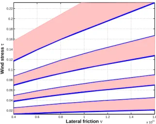
Primeau [46] showed that, in large basins comparable in size with the North Atlantic, there is not only one but a set of successive pitchfork bifurcations. One supercritical pitchfork bifurcation, associated with the destabilization of antisymmetric flows, is followed generically by a subcritical one, associated this time with a stabilization of antisymmetric flows (modulo high-frequency instabilities) [45]. As a matter of fact, this phenomenon appears to be a consequence of the spectral behavior of the 2-D Euler equations [47], and hence of the closely related barotropic QG model in bounded domains.

Remarkably, this scenario repeats itself as the nonlinearity increases, but now higher wavenumbers are involved in physical space. Simonnet [45] showed that this was also the case for gyre modes and the corresponding dynamics induced by global bifurcations: the low-frequency dynamics is quantized as the jet stream extends further eastward into the basin, due to the increased forcing and nonlinearity. Figure 5 illustrates this situation: two

0.4 0.6 0.8 1 1.2 1.4 1.6 x 1011 0.02 0.04 0.06 0.08 0.1 0.12 0.14 0.16 0.18 0.2 0.22 Wind stress τ Lateral friction ν

Figure 5: Two-parameter plane, with the wind-stress intensity τ vs. the eddy-viscosity coefficient ν: the curves indicate the locations of supercritical and subcritical pitchfork bifurcations. Each band is associated with a different wavenumber and timescale (from [45]).

families of regimes can be identified, the colored bands correspond to (supercritical) regimes driven by the gyre modes, the others to (subcritical) regimes driven by the eddies. Note that this scenario is also robust to perturbing the problem’s symmetry.

The theory appears therewith to be fairly complete for barotropic, single-layer models of the double-gyre circulation. In baroclinic models, with two or more active layers of different density, baroclinic instabilities [10, 13, 17, 18, 19, 25, 34, 41, 43, 44] surely play a fundamental role, as they do in the observed dynamics of the oceans. However, it is not known to what extent baroclinic instabilities can destroy gyre-mode dynamics. The difficulty lies in a deeper

understanding of the so-called rectification process [48], which arises from the nonzero mean effect of the baroclinic component of the flow.

Roughly speaking, rectification drives the dynamics far away from any steady states. In this situation, dynamical systems theory cannot be used as an explanation of complex, observed behavior resulting from successive bifurcations that are rooted in a simple steady state. Other tools from statistical mechanics and nonequilibrium thermodynamics should, therefore, be considered [49, 50, 51, 52]. Combining these tools with those of the successive-bifurcation approach may eventually lead to a more general and complete physical charac-terization of gyre modes in realistic models.

3

Climate-change projections and random dynamical

sys-tems

As discussed in Section 1, the climate system’s internal low-frequency variability is not the only cause for the uncertainties in projecting its future evolution. In this section, we address more generally these uncertainties and present a novel approach for treating them. To do so, we start with some simple ideas about deterministic vs. stochastic modeling.

3.1

Motivation

Many physical phenomena can be modeled by deterministic evolution equations. Dynamical systems theory is essentially a geometric approach for studying the asymptotic properties of solutions to such equations in phase space. Pioneered by H. Poincar´e [53], this theory took major strides over the last fifty years. The extent to which a particular dynamical system or class of such systems could adequately reflect those of the natural phenomena of interest is still an open question, though. Some concept of model robustness seems of the essence in lending credence to the physical relevance of a mathematical or numerical result.

In this context, Andronov and Pontryagin [54] took a major step toward classifying dy-namical systems, by introducing the concept of structural stability. This topological concept essentially stipulates that there exist a one-to-one continuous change of variables, called homeomorphism, that transforms the phase portrait of a system into that of another one. Closely related to this concept is the notion of hyperbolicity introduced by Smale [55]. A system is hyperbolic if, (very) loosely speaking, its limit set can be continuously decomposed into contracting and expanding invariant sets; see [56] for more rigorous definitions.

A very simple example is the phase portrait in the neighborhood of a fixed point of saddle type. In this case, the Hartman-Grobman theorem states that the dynamics in this neighborhood is structurally stable. The converse statement, i.e. whether structural stability implies hyperbolicity, is still an open question; it is true in the C1_{setting for diffeomorphisms}

that satisfy Axiom A and the strong transversality condition [57, 58, 59, 60]. The concepts and tools of bifurcation theory are well grounded in the setting of hyperbolic dynamics. Problems with hyperbolicity and bifurcations arise, however, when one deals with much more complicated limit sets.

Hyperbolicity was introduced initially to help pursue the “dream” to find an open and dense set of dynamical systems that are structurally stable: i.e. systems that even when perturbed slightly preserve the same (homeomorphic) dynamics. Smale conjectured that hyperbolic systems form an open and dense set in the space of all C1_{dynamical systems. If}

this conjecture were true then, by density and robustness, hyperbolicity would be typical of dynamics. Unfortunately, though, this conjecture is only true for one-dimensional dynamics and flows on disks and surfaces [61]. Smale himself found several counterexamples to his

conjecture [62]. One famous example is due to Newhouse [63] and another one is given by the Lorenz attractor [64]. Newhouse was able to generate open sets of nonhyperbolic diffeomorphisms using homoclinic tangencies. For the physicist, it is even more striking that the famous Lorenz attractor [65] is structurally unstable. Families of Lorenz attractors, classified by topological type, are not even countable [66].

Nonhyperbolic chaos appears, therefore, to be a severe obstacle to any “easy” classifi-cation of dynamic behavior. As mentioned by Palis [60], Kolmogorov already suggested at the end of the sixties that “the global study of dynamical systems could not go very far without the use of new additional mathematical tools, like probabilistic ones.” Once more, Kolmogorov showed prophetic insight, and nowadays the concept of stochastic stability is an important tool in the study of genericity and robustness for dynamical systems. To replace the failed program of classifying dynamical systems based on structural stability and hy-perbolicity, Palis [60] formulated what is now called the global conjecture: systems having only finitely many attractors (chaotic or periodic sinks) – such that (i) the union of their basins has total Lebesgue probability, and (ii) they are stochastically stable in their basins of attraction – are dense in the Cr_{, r ≥ 1 topology. A system is stochastically stable if its}

Sinai-Ruelle-Bowen (SRB) measure [67] is stable with respect to stochastic perturbations; the SRB measure is given by limn→∞n1

P

iδzi, with zi being the successive iterates of the dynamics, and it corresponds intuitively to allowing the entire phase space to flow onto the attractor [68].

Stochastic stability favors metric approaches and is fundamentally based on ergodic the-ory. We would like to consider a more geometric approach, which can provide a coarser, more robust classification of GCMs and their climate-change projections. We propose, therefore, such a geometric approach, based on concepts from the rapidly growing field of random dynamical systems (RDS), as developed by L. Arnold [16] and his “Bremen group,” among others. RDS in general describe the behavior of dynamical systems subject to external sto-chastic forcing. The tools of RDS theory have been developed to help study the geometric properties of stochastic differential equations (SDEs). In some sense, they are the stochastic counterpart of the geometric theory of ordinary differential equations (ODEs). This approach provides a rigorous mathematical framework for a stochastic form of robustness, while the more traditional, topological concepts do not seem to be appropriate.

3.2

RDS, random attractors, and robust classification

A central idea in developing stochastic parametrizations for GCMs is that these are aimed at compensating for our lack of knowledge in the best way possible [69, 70, 71, 72, 73, 74]. Since such parametrizations deal typically with small space scales, the underlying assumption is that the associated time scales are also much shorter than the scales of interest and therefore the time correlation of the phenomena being parametrized is negligibly small. Bearing this in mind, stochastic parametrizations essentially transform a deterministic autonomous system into a nonautonomous one, subject to random forcing.

The nonautonomous character of a dynamical system immediately raises a technical difficulty. Indeed, the classical notion of attractor is no longer valid since any object in phase space is “moving” with time and the natural concept of forward asymptotics is meaningless. One needs therefore another concept of attractor. In the deterministic nonautonomous framework, this concept corresponds to the pullback attractor [75] that we present below.

3.2.1 Framework and objectives

Before defining the notion of pullback attractor, let us recall some basic important facts about nonautonomous dynamical systems. Consider the nonautonomous ODE ˙x = f (t, x) on a Banach space X. Rigorously speaking, we cannot associate a dynamical system acting on X with a nonautonomous ODE; nevertheless, in the case of unique solvability of the initial-value problem, we can introduce a two-parameter family of operators {S(t, s)}t≥s

acting on X with s, t ∈ R, such that S(t, s)x(t) = x(s), t ≥ s, where x(t) is the solution of the Cauchy problem with initial data x(s). This family of operators satisfies S(s, s) = IdX,

for all s ∈ R and S(t, τ ) ◦ S(τ, s) = S(t, s) for all t ≥ τ ≥ s, s ∈ R. This family of operators is called a “process” by Sell [76]. It extends the classical notion of resolvent from autonomous to nonautonomous linear ODEs.

We can now define the pullback attractor as simply the family of invariant sets {A(t)} that satisfy for every t ∈ R :

lim

s→−∞dist (S(t, s)x0, A(t)) = 0, for all x0∈ X.

The idea of “pullback” attraction does not involve running time backwards; it corresponds instead to the idea that measurements in an experiment performed at present time t, started some time in the past, at a time s < t: the experiment has been running for long enough, and we are thus looking now at an “attracting state.” Note that there exists several ways of defining a pullback attractor — the one retained here is a local one (cf. [75] and references therein); for further information on nonautonomous dynamical systems in general, see [77]. We shall use next the concept of pullback attractor to define a random attractor, but need first to define an RDS. We denote by T one of the following sets: N, Z, R+_{, R. Let}

(X, B) be a measurable phase space, and (Ω, F, P, (θ(t))t∈T) be a metric dynamical system

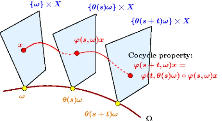
i.e. a flow in the probability space (Ω, F, P), such that (t, ω) 7→ θ(t)ω is measurable and θ(t) : Ω → Ω is measure preserving, θ(t)P = P. Let ϕ : T × Ω × X → X, (t, ω, x) 7→ ϕ(t, ω)x, be a mapping with the following two properties:

(R1): ϕ(0, ω) = IdX, and

(R2) (the cocycle property): For all s, t ∈ T and all ω ∈ Ω,

ϕ(t + s, ω) = ϕ(t, θ(s)ω) ◦ ϕ(s, ω).

If ϕ is measurable, then it is called a measurable RDS over θ. If in addition, X is a topological space (respectively a Banach space), and ϕ satisfies (t, ω) 7→ ϕ(t, ω)x continuous (resp. Ck_{, 1 ≤ k ≤ ∞) for all (t, ω) ∈ T × Ω, then ϕ is called a continuous (resp. C}k_{) RDS}

over the flow θ. If so, then

(ω, x) 7→ Θ(t)(x, ω) := (θ(t)ω, ϕ(t, ω)x),

is a (measurable) flow on Ω × X, the so-called skew-product of θ and ϕ. In the sequel, we shall use the terms “RDS” or “cocycles” synonymously. The choice of a metric dynamical system θ is a crucial step in this set-up and is dictated by external constraints specific to the problem at hand; as far as stochastic classification is concerned, it does play an important role [78].

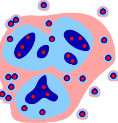
In this stochastic context, the concept of random attractor is a natural and straightfor-ward extension of the definition of pullback attractor, in which Sell’s [76] process is replaced by a cocycle, cf. Fig. 6, and A now depends on the realization ω of the noise, so that we have

a family of random attractors A(ω), cf. Fig. 7. Roughly speaking, for a fixed realization of the noise, one “rewinds” the noise back to t → −∞ and lets the experiment evolve (forward in time) towards a possibly attracting set A(ω); the driving system θ enables one to do this rewinding without changing the statistics, cf. Figs. 6 and 7.

Figure 6: Random dynamical systems (RDS) viewed as a flow on the bundle X × Ω = “dynamical space” × “probability space.” For a given position x and realization ω, the RDS ϕ is such that Θ(t)(x, ω) = (θ(t)ω, ϕ(t, ω)x) is a flow on the bundle.

{θ( )ω}t xX {ω}xX θ( )ωt A( )ω ϕ( ,ω) t A( )=ω A( )θ( )ωt Ω ω Pullback attraction to A( )ω 2 θ(−τ )ω θ(−τ )ω1 θ(−τ )ω) B( θ(−τ )ω) B( ₂ 1

Figure 7: Schematic diagram of a random attractor A(ω), where ω ∈ Ω is a fixed realization of the noise. To be attracting, ∀B ∈ B, with B ⊂ 2X _{being a collection of subsets of X,}

one must have limt→+∞dist(B(θ(−t)ω), A(ω)) = 0 with B(θ(−t)ω) := ϕ(t, θ(−t)ω)B; to be

invariant, one must have ϕ(t, ω)A(ω) = A(θ(t)ω). This definition depends strongly on B; see [80] for more details.

Other notions of attractor can be defined in the stochastic context, in particular based on the original SDE; see [79] or [80] for a discussion on this topic. The present definition, though, will serve us well.

Having defined the concepts of RDS and random attractors, we now introduce the notion of stochastic conjugacy or equivalence. This notion enables one to rigourously compare two distinct RDS and it is defined as follows: two cocycles ϕ1(ω, t) and ϕ2(ω, t) are conjugated

such that h(ω)(0) = 0 and

ϕ1(ω, t) = h(θ(t)ω)−1◦ ϕ2(ω, t) ◦ h(ω). (3.1)

Stochastic equivalence extends classic topological conjugacy to the bundle space X × Ω, where there exists a one-to-one (stochastic) change of variables that transforms one phase portrait into the other.

Returning now to our main objective, suppose for instance that one is presented with results from two distinct GCMs, say two probability distributions functions (PDFs) of the temperature or precipitation in a given area. These two PDFs are generated, typically, by an ensemble of each GCM’s simulations, as described in the introduction, and they are likely to differ in their spatial pattern. To ascertain the physical significance of this discrepancy, one needs to know how each GCM result varies as either a parametrization or a parameter value are changed.

In order to consider the difficult question of why GCM responses might differ, one idea is to investigate the structure of the space of all GCMs. We mean therewith the space of all deterministic GCMs, when their stochastic parametrizations are switched off. We know, by now, from experience with GCM results over several decades – including the four IPCC assessment reports [2, 3, 4] and the climateprediction.net exercise [5, 6, 7] – that there is enormous scatter in this space; see also [81, 82]. Our question, therefore, is: can we achieve a genuine, robust classification of GCMs when stochastic parametrizations are used and for a given level of the noise?

As mentioned in Section 3.1, such a classification is not feasible by restricting ourself to deterministic systems and topological concepts. As one switches on stochastic parametriza-tions [69, 70, 71, 72, 73, 74], the situation might change, and hopefully improve, dramatically. Roughly speaking, as the level of the noise becomes very large, it is expected that the mod-els’ deterministic behavior will be completely destroyed, and all results would cluster into one huge, diffuse clump. We would like, therefore, to investigate how a classification based on stochastic equivalence evolves as the level of the noise or the stochastic parametrizations change. As the noise tends to zero, do we recover the “granularity” of the set of all deter-ministic dynamical systems? This idea is schematically represented in Fig. 8: for a given level of the noise, we expect the space of all GCMs to be decomposed into a possibly finite number of classes. Within one of these classes, all the GCMs are topologically equivalent in the stochastic sense defined above; see Eq. (3.1).

Serious difficulties might arise in this program, due to the presence of nonhyperbolic chaos in climate models. Several researches have pointed out that even the characteristics of noisy hyperbolic chaos may strongly depend on the intensity of the noise and its statistics [84, 85, 86, 87].

Such issues go well beyond the setting of this paper and are left for further investigation. Much more modestly, we will study here whether, in certain very simple cases, the conjectural view of Fig. 8 might be relevant for some dynamical systems that are “metaphors” of climate dynamics. The following subsection is dedicated to the study of such a metaphorical object, namely the Arnol’d circle map.

3.2.2 The stochastically perturbed circle map

To go further than our pictorial view of stochastic classification for GCMs in Fig. 8, we study now the effect of noise on a family of circle diffeomorphisms. This toy model exhibits two interesting features for our purpose. The first one is that the two-parameter family {Fτ,ǫ} defined by Eq. (3.2) below exhibits an infinite number of topological classes (cf. chap

✁ ✁ ✁ ✁ ✁ ✁ ✁ ✁ ✁ ✁ ✁ ✁ ✁ ✁ ✁ ✁ ✁ ✁ ✁ ✁ ✁ ✁ ✁ ✁ ✁ ✁ ✁ ✁ ✁ ✁ ✁ ✁ ✁ ✁ ✁ ✁ ✁ ✁ ✁ ✁ ✁ ✁ ✁ ✁ ✁ ✁ ✁ ✁ ✁ ✁ ✁ ✁ ✁ ✁ ✁ ✁ ✁ ✁ ✁ ✁ ✁ ✁ ✁ ✁ ✁ ✁ ✁ ✁ ✁ ✁ ✁ ✁ ✁ ✁ ✁ ✁ ✁ ✁ ✁ ✁ ✁ ✁ ✁ ✁ ✁ ✁ ✁ ✁ ✁ ✁ ✁ ✁ ✁ ✁ ✁ ✁ ✁ ✁ ✁ ✁ ✁ ✁ ✁ ✁ ✁ ✁ ✁ ✁ ✁ ✁ ✁ ✁ ✁ ✁ ✁ ✁ ✁ ✁ ✁ ✁ ✁ ✁ ✁ ✁ ✁ ✁ ✁ ✁ ✁ ✁ ✁ ✁ ✁ ✁ ✁ ✁ ✁ ✁ ✁ ✁ ✁ ✁ ✁ ✁ ✁ ✁ ✁ ✁ ✁ ✁ ✁ ✁ ✁ ✁ ✁ ✁ ✁ ✁ ✁ ✁ ✁ ✁ ✁ ✁ ✁ ✁ ✁ ✁ ✁ ✁ ✁ ✁ ✁ ✁ ✁ ✁ ✁ ✁ ✁ ✁ ✁ ✁ ✁ ✁ ✁ ✁ ✁ ✁ ✁ ✁ ✁ ✁ ✁ ✁ ✁ ✁ ✁ ✁ ✁ ✁ ✁ ✁ ✁ ✁ ✁ ✁ ✁ ✁ ✁ ✁ ✁ ✁ ✁ ✁ ✁ ✁ ✁ ✁ ✁ ✁ ✁ ✁ ✁ ✁ ✁ ✁ ✁ ✁ ✁ ✁ ✁ ✁ ✁ ✁ ✁ ✁ ✁ ✁ ✁ ✁ ✁ ✁ ✁ ✁ ✁ ✁ ✁ ✁ ✁ ✁ ✁ ✁ ✁ ✁ ✁ ✁ ✁ ✁ ✁ ✁ ✁ ✁ ✁ ✁ ✁ ✁ ✁ ✁ ✁ ✁ ✁ ✁ ✁ ✁ ✁ ✁ ✁ ✁ ✁ ✁ ✁ ✁ ✁ ✁ ✁ ✁ ✁ ✁ ✁ ✁ ✁ ✁ ✁ ✁ ✁ ✁ ✁ ✁ ✁ ✁ ✁ ✁ ✁ ✁ ✁ ✁ ✁ ✁ ✁ ✁ ✁ ✁ ✁ ✁ ✁ ✁ ✁ ✁ ✁ ✁ ✁ ✁ ✁ ✁ ✁ ✁ ✁ ✁ ✁ ✁ ✁ ✁ ✁ ✁ ✁ ✁ ✁ ✁ ✁ ✁ ✁ ✁ ✁ ✁ ✁ ✁ ✁ ✁ ✁ ✁ ✁ ✁ ✁ ✁ ✁ ✁ ✁ ✁ ✁ ✁ ✁ ✁ ✁ ✁ ✁ ✁ ✁ ✁ ✁ ✁ ✁ ✁ ✁ ✁ ✁ ✁ ✁ ✁ ✁ ✁ ✁ ✁ ✁ ✁ ✁ ✁ ✁ ✁ ✁ ✁ ✁ ✁ ✁ ✁ ✁ ✁ ✁ ✁ ✁ ✁ ✁ ✁ ✁ ✁ ✁ ✁ ✁ ✁ ✁ ✁ ✁ ✁ ✁ ✁ ✁ ✁ ✁ ✁ ✁ ✁ ✁ ✁ ✁ ✁ ✁ ✁ ✁ ✁ ✁ ✁ ✁ ✁ ✁ ✁ ✁ ✁ ✁ ✁ ✁ ✁ ✁ ✁ ✁ ✁ ✁ ✁ ✁ ✁ ✁ ✁ ✁ ✁ ✁ ✁ ✁ ✁ ✁ ✁ ✁ ✁ ✁ ✁ ✁ ✁ ✁ ✁ ✁ ✁ ✁ ✁ ✁ ✁ ✁ ✁ ✁ ✁ ✁ ✁ ✁ ✁ ✁ ✁ ✁ ✁ ✁ ✁ ✁ ✁ ✁ ✁ ✁ ✁ ✁ ✁ ✁ ✁ ✁ ✁ ✁ ✁ ✁ ✁ ✁ ✁ ✁ ✁ ✁ ✁ ✁ ✁ ✁ ✁ ✁ ✁ ✁ ✁ ✁ ✁ ✁ ✁ ✁ ✁ ✁ ✁ ✁ ✁ ✁ ✁ ✁ ✁ ✁ ✁ ✁ ✁ ✁ ✁ ✁ ✁ ✁ ✁ ✁ ✁ ✁ ✁ ✁ ✁ ✁ ✁ ✁ ✁ ✁ ✁ ✁ ✁ ✁ ✁ ✁ ✁ ✁ ✁ ✁ ✁ ✁ ✁ ✁ ✁ ✁ ✁ ✁ ✁ ✁ ✁ ✁ ✁ ✁ ✁ ✁ ✁ ✁ ✁ ✁ ✁ ✁ ✁ ✁ ✁ ✁ ✁ ✁ ✁ ✁ ✁ ✁ ✁ ✁ ✁ ✁ ✁ ✁ ✁ ✁ ✁ ✁ ✁ ✁ ✁ ✁ ✁ ✁ ✁ ✁ ✁ ✁ ✁ ✁ ✁ ✁ ✁ ✁ ✁ ✁ ✁ ✁ ✁ ✁ ✁ ✁ ✁ ✁ ✁ ✁ ✁ ✁ ✁ ✁ ✁ ✁ ✁ ✁ ✁ ✁ ✁ ✁ ✁ ✁ ✁ ✁ ✁ ✁ ✁ ✁ ✁ ✁ ✁ ✁ ✁ ✁ ✁ ✁ ✁ ✁ ✁ ✁ ✁ ✁ ✁ ✁ ✁ ✁ ✁ ✁ ✁ ✁ ✁ ✁ ✁ ✁ ✁ ✁ ✁ ✁ ✁ ✁ ✁ ✁ ✁ ✁ ✁ ✁ ✁ ✁ ✁ ✁ ✁ ✁ ✁ ✁ ✁ ✁ ✁ ✁ ✁ ✁ ✁ ✁ ✁ ✁ ✁ ✁ ✁ ✁ ✁ ✁ ✁ ✁ ✁ ✁ ✁ ✁ ✁ ✁ ✁ ✁ ✁ ✁ ✁ ✁ ✁ ✁ ✁ ✁ ✁ ✁ ✁ ✁ ✁ ✁ ✁ ✁ ✁ ✁ ✁ ✁ ✁ ✁ ✁ ✁ ✁ ✁ ✁ ✁ ✁ ✁ ✁ ✁ ✁ ✁ ✁ ✁ ✁ ✁ ✁ ✁ ✁ ✁ ✁ ✁ ✁ ✁ ✁ ✁ ✁ ✁ ✁ ✁ ✁ ✁ ✁ ✁ ✁ ✁ ✁ ✁ ✁ ✁ ✁ ✁ ✁ ✁ ✁ ✁ ✁ ✁ ✁ ✁ ✁ ✁ ✁ ✁ ✁ ✁ ✁ ✁ ✁ ✁ ✁ ✁ ✁ ✁ ✁ ✁ ✁ ✁ ✁ ✁ ✁ ✁ ✁ ✁ ✁ ✁ ✁ ✁ ✁ ✁ ✁ ✁ ✁ ✁ ✁ ✁ ✁ ✁ ✁ ✁ ✁ ✁ ✁ ✁ ✁ ✁ ✁ ✁ ✁ ✁ ✁ ✁ ✁ ✁ ✁ ✁ ✁ ✁ ✁ ✁ ✁ ✁ ✁ ✁ ✁ ✁ ✁ ✁ ✁ ✁ ✁ ✁ ✁ ✁ ✁ ✁ ✁ ✁ ✁ ✁ ✁ ✁ ✁ ✁ ✁ ✁ ✁ ✁ ✁ ✁ ✁ ✁ ✁ ✁ ✁ ✁ ✁ ✁ ✁ ✁ ✁ ✁ ✁ ✁ ✁ ✁ ✁ ✁ ✁ ✁ ✁ ✁ ✁ ✁ ✁ ✁ ✁ ✁ ✁ ✁ ✁ ✁ ✁ ✁ ✁ ✁ ✁ ✁ ✁ ✁ ✁ ✁ ✁ ✁ ✁ ✁ ✁ ✁ ✁ ✁ ✁ ✁ ✁ ✁ ✁ ✁ ✁ ✁ ✁ ✁ ✁ ✁ ✁ ✁ ✁ ✁ ✁ ✁ ✁ ✁ ✁ ✁ ✁ ✁ ✁ ✁ ✁ ✁ ✁ ✁ ✁ ✁ ✁ ✁ ✁ ✁ ✁ ✁ ✁ ✁ ✁ ✁ ✁ ✁ ✁ ✁ ✁ ✁ ✁ ✁ ✁ ✁ ✁ ✁ ✁ ✁ ✁ ✁ ✁ ✁ ✁ ✁ ✁ ✁ ✁ ✁ ✁ ✁ ✁ ✁ ✁ ✁ ✁ ✁ ✁ ✁ ✁ ✁ ✁ ✁ ✁ ✁ ✁ ✁ ✁ ✁ ✁ ✁ ✁ ✁ ✁ ✁ ✁ ✁ ✁ ✁ ✁ ✁ ✁ ✁ ✁ ✁ ✁ ✁ ✁ ✁ ✁ ✁ ✁ ✁ ✁ ✁ ✁ ✁ ✁ ✁ ✁ ✁ ✁ ✁ ✁ ✁ ✁ ✁ ✁ ✁ ✁ ✁ ✁ ✁ ✁ ✁ ✁ ✁ ✁ ✁ ✁ ✁ ✁ ✁ ✁ ✁ ✁ ✁ ✁ ✁ ✁ ✁ ✁ ✁ ✁ ✁ ✁ ✁ ✁ ✁ ✁ ✁ ✁ ✁ ✁ ✁ ✁ ✁ ✁ ✁ ✁ ✁ ✁ ✁ ✁ ✁ ✁ ✁ ✁ ✁ ✁ ✁ ✁ ✁ ✁ ✁ ✁ ✁ ✁ ✁ ✁ ✁ ✁ ✁ ✁ ✁ ✁ ✁ ✁ ✁ ✁ ✁ ✁ ✁ ✁ ✁ ✁ ✁ ✁ ✁ ✁ ✁ ✁ ✁ ✁ ✁ ✁ ✁ ✁ ✁ ✁ ✁ ✁ ✁ ✁ ✁ ✁ ✁ ✁ ✁ ✁ ✁ ✁ ✁ ✁ ✁ ✁ ✁ ✁ ✁ ✁ ✁ ✁ ✁ ✁ ✁ ✁ ✁ ✁ ✁ ✁ ✁ ✁ ✁ ✁ ✁ ✁ ✁ ✁ ✁ ✁ ✁ ✁ ✁ ✁ ✁ ✁ ✁ ✁ ✁ ✁ ✁ ✁ ✁ ✁ ✁ ✁ ✁ ✁ ✁ ✁ ✁ ✁ ✁ ✁ ✁ ✁ ✁ ✁ ✁ ✁ ✁ ✁ ✁ ✁ ✁ ✁ ✁ ✁ ✁ ✁ ✁ ✁ ✁ ✁ ✁ ✁ ✁ ✁ ✁ ✁ ✁ ✁ ✁ ✁ ✁ ✁ ✁ ✁ ✁ ✁ ✁ ✁ ✁ ✁ ✁ ✁ ✁ ✁ ✁ ✁ ✁ ✁ ✁ ✁ ✁ ✁ ✁ ✁ ✁ ✁ ✁ ✁ ✁ ✁ ✁ ✁ ✁ ✁ ✁ ✁ ✁ ✁ ✁ ✁ ✁ ✁ ✁ ✁ ✁ ✁ ✁ ✁ ✁ ✁ ✁ ✁ ✁ ✁ ✁ ✁ ✁ ✁ ✁ ✁ ✁ ✁ ✁ ✁ ✁ ✁ ✁ ✁ ✁ ✁ ✁ ✁ ✁ ✁ ✁ ✁ ✁ ✁ ✁ ✁ ✁ ✁ ✁ ✁ ✁ ✁ ✁ ✁ ✁ ✁ ✁ ✁ ✁ ✁ ✁ ✁ ✁ ✁ ✁ ✁ ✁ ✁ ✁ ✁ ✁ ✁ ✁ ✁ ✁ ✁ ✁ ✁ ✁ ✁ ✁ ✁ ✁ ✁ ✁ ✁ ✁ ✁ ✁ ✁ ✁ ✁ ✁ ✁ ✁ ✁ ✁ ✁ ✁ ✁ ✁ ✁ ✁ ✁ ✁ ✁ ✁ ✁ ✁ ✁ ✁ ✁ ✁ ✁ ✁ ✁ ✁ ✁ ✁ ✁ ✁ ✁ ✁ ✁ ✁ ✁ ✁ ✁ ✁ ✁ ✁ ✁ ✁ ✁ ✁ ✁ ✁ ✁ ✁ ✁ ✁ ✁ ✁ ✁ ✁ ✁ ✁ ✁ ✁ ✁ ✁ ✁ ✁ ✁ ✁ ✁ ✁ ✁ ✁ ✁ ✁ ✁ ✁ ✁ ✁ ✁ ✁ ✁ ✁ ✁ ✁ ✁ ✁ ✁ ✁ ✁ ✁ ✁ ✁ ✁ ✁ ✁ ✁ ✁ ✁ ✁ ✁ ✁ ✁ ✁ ✁ ✁ ✁ ✁ ✁ ✁ ✁ ✁ ✁ ✁ ✁ ✁ ✁ ✁ ✁ ✁ ✁ ✁ ✁ ✁ ✁ ✁ ✁ ✁ ✁ ✁ ✁ ✁ ✁ ✁ ✁ ✁ ✁ ✁ ✁ ✁ ✁ ✁ ✁ ✁ ✁ ✁ ✁ ✁ ✁ ✁ ✁ ✁ ✁ ✁ ✁ ✁ ✁ ✁ ✁ ✁ ✁ ✁ ✁ ✁ ✁ ✁ ✁ ✁ ✁ ✁ ✁ ✁ ✁ ✁ ✁ ✁ ✁ ✁ ✁ ✁ ✁ ✁ ✁ ✁ ✁ ✁ ✁ ✁ ✁ ✁ ✁ ✁ ✁ ✁ ✁ ✁ ✁ ✁ ✁ ✁ ✂ ✂ ✂ ✂ ✂ ✂ ✂ ✂ ✂ ✂ ✂ ✂ ✂ ✂ ✂ ✂ ✂ ✂ ✂ ✂ ✂ ✂ ✂ ✂ ✂ ✂ ✂ ✂ ✂ ✂ ✂ ✂ ✂ ✂ ✂ ✂ ✂ ✂ ✂ ✂ ✂ ✂ ✂ ✂ ✂ ✂ ✂ ✂ ✂ ✂ ✂ ✂ ✂ ✂ ✂ ✂ ✂ ✂ ✂ ✂ ✂ ✂ ✂ ✂ ✂ ✂ ✂ ✂ ✂ ✂ ✂ ✂ ✂ ✂ ✂ ✂ ✂ ✂ ✂ ✂ ✂ ✂ ✂ ✂ ✂ ✂ ✂ ✂ ✂ ✂ ✂ ✂ ✂ ✂ ✂ ✂ ✂ ✂ ✂ ✂ ✂ ✂ ✂ ✂ ✂ ✂ ✂ ✂ ✂ ✂ ✂ ✂ ✂ ✂ ✂ ✂ ✂ ✂ ✂ ✂ ✂ ✂ ✂ ✂ ✂ ✂ ✂ ✂ ✂ ✂ ✂ ✂ ✂ ✂ ✂ ✂ ✂ ✂ ✂ ✂ ✂ ✂ ✂ ✂ ✂ ✂ ✂ ✂ ✂ ✂ ✂ ✂ ✂ ✂ ✂ ✂ ✂ ✂ ✂ ✂ ✂ ✂ ✂ ✂ ✂ ✂ ✂ ✂ ✂ ✂ ✂ ✂ ✂ ✂ ✂ ✂ ✂ ✂ ✂ ✂ ✂ ✂ ✂ ✂ ✂ ✂ ✂ ✂ ✂ ✂ ✂ ✂ ✂ ✂ ✂ ✂ ✂ ✂ ✂ ✂ ✂ ✂ ✂ ✂ ✂ ✂ ✂ ✂ ✂ ✂ ✂ ✂ ✂ ✂ ✂ ✂ ✂ ✂ ✂ ✂ ✂ ✂ ✂ ✂ ✂ ✂ ✂ ✂ ✂ ✂ ✂ ✂ ✂ ✂ ✂ ✂ ✂ ✂ ✂ ✂ ✂ ✂ ✂ ✂ ✂ ✂ ✂ ✂ ✂ ✂ ✂ ✂ ✂ ✂ ✂ ✂ ✂ ✂ ✂ ✂ ✂ ✂ ✂ ✂ ✂ ✂ ✂ ✂ ✂ ✂ ✂ ✂ ✂ ✂ ✂ ✂ ✂ ✂ ✂ ✂ ✂ ✂ ✂ ✂ ✂ ✂ ✂ ✂ ✂ ✂ ✂ ✂ ✂ ✂ ✂ ✂ ✂ ✂ ✂ ✂ ✂ ✂ ✂ ✂ ✂ ✂ ✂ ✂ ✂ ✂ ✂ ✂ ✂ ✂ ✂ ✂ ✂ ✂ ✂ ✂ ✂ ✂ ✂ ✂ ✂ ✂ ✂ ✂ ✂ ✂ ✂ ✂ ✂ ✂ ✂ ✂ ✂ ✂ ✂ ✂ ✂ ✂ ✂ ✂ ✂ ✄ ✄ ✄ ✄ ✄ ✄ ✄ ✄ ✄ ✄ ✄ ✄ ✄ ✄ ✄ ✄ ✄ ✄ ✄ ✄ ✄ ✄ ✄ ✄ ✄ ✄ ✄ ✄ ✄ ✄ ✄ ✄ ✄ ✄ ✄ ✄ ✄ ✄ ✄ ✄ ✄ ✄ ✄ ✄ ✄ ✄ ✄ ✄ ✄ ✄ ✄ ✄ ✄ ✄ ✄ ✄ ✄ ✄ ✄ ✄ ✄ ✄ ✄ ✄ ✄ ✄ ✄ ✄ ✄ ✄ ✄ ✄ ✄ ✄ ✄ ✄ ✄ ✄ ✄ ✄ ✄ ✄ ✄ ✄ ✄ ✄ ✄ ✄ ✄ ✄ ✄ ✄ ✄ ✄ ✄ ✄ ✄ ✄ ✄ ✄ ✄ ✄ ✄ ✄ ✄ ✄ ✄ ✄ ✄ ✄ ✄ ✄ ✄ ✄ ✄ ✄ ✄ ✄ ✄ ✄ ✄ ✄ ✄ ✄ ✄ ✄ ✄ ✄ ✄ ✄ ✄ ✄ ✄ ✄ ✄ ✄ ✄ ✄ ✄ ✄ ✄ ✄ ✄ ✄ ✄ ✄ ✄ ✄ ✄ ✄ ✄ ✄ ✄ ✄ ✄ ✄ ✄ ✄ ✄ ✄ ✄ ✄ ✄ ✄ ✄ ✄ ✄ ✄ ✄ ✄ ✄ ✄ ✄ ✄ ✄ ✄ ✄ ✄ ✄ ✄ ✄ ✄ ✄ ✄ ✄ ✄ ✄ ✄ ✄ ✄ ✄ ✄ ✄ ✄ ✄ ✄ ✄ ✄ ✄ ✄ ✄ ✄ ✄ ✄ ✄ ✄ ✄ ✄ ✄ ✄ ✄ ✄ ✄ ✄ ✄ ✄ ✄ ✄ ✄ ✄ ✄ ✄ ✄ ✄ ✄ ✄ ✄ ✄ ✄ ✄ ✄ ✄ ✄ ✄ ✄ ✄ ✄ ✄ ✄ ✄ ✄ ✄ ✄ ✄ ✄ ✄ ✄ ✄ ✄ ✄ ✄ ✄ ✄ ✄ ✄ ✄ ✄ ✄ ✄ ✄ ✄ ✄ ✄ ✄ ✄ ✄ ✄ ✄ ✄ ✄ ✄ ✄ ✄ ✄ ✄ ✄ ✄ ✄ ✄ ✄ ✄ ✄ ✄ ✄ ✄ ✄ ✄ ✄ ✄ ✄ ✄ ✄ ✄ ✄ ✄ ✄ ✄ ✄ ✄ ✄ ✄ ✄ ✄ ✄ ✄ ✄ ✄ ✄ ✄ ✄ ✄ ✄ ✄ ✄ ✄ ✄ ✄ ✄ ✄ ✄ ✄ ✄ ☎ ☎ ☎ ☎ ☎ ☎ ☎ ☎ ☎ ☎ ☎ ☎ ☎ ☎ ☎ ☎ ☎ ☎ ☎ ☎ ☎ ☎ ☎ ☎ ☎ ☎ ☎ ☎ ☎ ☎ ☎ ☎ ☎ ☎ ☎ ☎ ☎ ☎ ☎ ☎ ☎ ☎ ☎ ☎ ☎ ☎ ☎ ☎ ☎ ☎ ☎ ☎ ☎ ☎ ☎ ☎ ☎ ☎ ☎ ☎ ☎ ☎ ☎ ☎ ☎ ☎ ☎ ☎ ☎ ☎ ☎ ☎ ☎ ☎ ☎ ☎ ☎ ☎ ☎ ☎ ☎ ☎ ☎ ☎ ☎ ☎ ☎ ☎ ☎ ☎ ☎ ☎ ☎ ☎ ☎ ☎ ☎ ☎ ☎ ☎ ☎ ☎ ☎ ☎ ☎ ☎ ☎ ☎ ☎ ☎ ☎ ☎ ☎ ☎ ☎ ☎ ☎ ☎ ☎ ☎ ☎ ☎ ☎ ☎ ☎ ☎ ☎ ☎ ☎ ☎ ☎ ☎ ☎ ☎ ☎ ☎ ☎ ☎ ☎ ☎ ☎ ☎ ☎ ☎ ☎ ☎ ☎ ☎ ☎ ☎ ☎ ☎ ☎ ☎ ☎ ☎ ☎ ☎ ☎ ☎ ☎ ☎ ☎ ☎ ☎ ☎ ☎ ☎ ☎ ☎ ☎ ☎ ☎ ☎ ☎ ☎ ☎ ☎ ☎ ☎ ☎ ☎ ☎ ☎ ☎ ☎ ☎ ☎ ☎ ☎ ☎ ☎ ☎ ☎ ☎ ☎ ☎ ☎ ☎ ☎ ☎ ☎ ☎ ☎ ☎ ☎ ☎ ☎ ☎ ☎ ☎ ☎ ☎ ☎ ☎ ☎ ☎ ☎ ☎ ☎ ☎ ☎ ☎ ☎ ☎ ☎ ☎ ☎ ☎ ☎ ☎ ☎ ☎ ☎ ☎ ☎ ☎ ☎ ☎ ☎ ☎ ☎ ☎ ☎ ☎ ☎ ☎ ☎ ☎ ☎ ☎ ☎ ☎ ☎ ☎ ☎ ☎ ☎ ☎ ☎ ☎ ☎ ☎ ☎ ☎ ☎ ☎ ☎ ☎ ☎ ☎ ☎ ☎ ☎ ☎ ☎ ☎ ☎ ☎ ☎ ☎ ☎ ☎ ☎ ☎ ☎ ☎ ☎ ☎ ☎ ☎ ☎ ☎ ☎ ☎ ☎ ☎ ✆ ✆ ✆ ✆ ✆ ✆ ✆ ✆ ✆ ✆ ✆ ✆ ✆ ✆ ✆ ✆ ✆ ✆ ✆ ✆ ✆ ✆ ✆ ✆ ✆ ✆ ✆ ✆ ✆ ✆ ✆ ✆ ✆ ✆ ✆ ✆ ✆ ✆ ✆ ✆ ✆ ✆ ✆ ✆ ✆ ✆ ✆ ✆ ✆ ✆ ✆ ✆ ✆ ✆ ✆ ✆ ✆ ✆ ✆ ✆ ✆ ✆ ✆ ✆ ✆ ✆ ✆ ✆ ✆ ✆ ✆ ✆ ✆ ✆ ✆ ✆ ✆ ✆ ✆ ✆ ✆ ✆ ✆ ✆ ✆ ✆ ✆ ✆ ✆ ✆ ✆ ✆ ✆ ✆ ✆ ✆ ✆ ✆ ✆ ✆ ✆ ✆ ✆ ✆ ✆ ✆ ✆ ✆ ✆ ✆ ✆ ✆ ✆ ✆ ✆ ✆ ✆ ✆ ✆ ✆ ✆ ✆ ✆ ✆ ✆ ✆ ✆ ✆ ✆ ✆ ✆ ✆ ✆ ✆ ✆ ✆ ✆ ✆ ✆ ✆ ✆ ✆ ✆ ✆ ✆ ✆ ✆ ✆ ✆ ✆ ✆ ✆ ✆ ✆ ✆ ✆ ✆ ✆ ✆ ✆ ✆ ✆ ✆ ✆ ✆ ✆ ✆ ✆ ✆ ✆ ✆ ✆ ✆ ✆ ✆ ✆ ✆ ✆ ✆ ✆ ✆ ✆ ✆ ✆ ✆ ✆ ✆ ✆ ✆ ✆ ✆ ✆ ✆ ✆ ✆ ✆ ✆ ✆ ✆ ✆ ✆ ✆ ✆ ✆ ✆ ✆ ✆ ✆ ✆ ✆ ✆ ✆ ✆ ✆ ✆ ✆ ✆ ✆ ✆ ✆ ✆ ✆ ✆ ✆ ✆ ✆ ✆ ✆ ✆ ✆ ✆ ✆ ✆ ✆ ✆ ✆ ✆ ✆ ✆ ✆ ✆ ✆ ✆ ✆ ✆ ✆ ✆ ✆ ✆ ✆ ✆ ✆ ✆ ✆ ✆ ✆ ✆ ✆ ✆ ✆ ✆ ✆ ✆ ✆ ✆ ✆ ✆ ✆ ✆ ✆ ✆ ✆ ✆ ✆ ✆ ✆ ✆ ✆ ✆ ✆ ✆ ✆ ✆ ✆ ✆ ✆ ✆ ✆ ✆ ✆ ✆ ✆ ✆ ✆ ✆ ✆ ✆ ✝ ✝ ✝ ✝ ✝ ✝ ✝ ✝ ✝ ✝ ✝ ✝ ✝ ✝ ✝ ✝ ✝ ✝ ✝ ✝ ✝ ✝ ✝ ✝ ✝ ✝ ✝ ✝ ✝ ✝ ✝ ✝ ✝ ✝ ✝ ✝ ✝ ✝ ✝ ✝ ✝ ✝ ✝ ✝ ✝ ✝ ✝ ✝ ✝ ✝ ✝ ✝ ✝ ✝ ✝ ✝ ✝ ✝ ✝ ✝ ✝ ✝ ✝ ✝ ✝ ✝ ✝ ✝ ✝ ✝ ✝ ✝ ✝ ✝ ✝ ✝ ✝ ✝ ✝ ✝ ✝ ✝ ✝ ✝ ✝ ✝ ✝ ✝ ✝ ✝ ✝ ✝ ✝ ✝ ✝ ✝ ✝ ✝ ✝ ✝ ✝ ✝ ✝ ✝ ✝ ✝ ✝ ✝ ✝ ✝ ✝ ✝ ✝ ✝ ✝ ✝ ✝ ✝ ✝ ✝ ✝ ✝ ✝ ✝ ✝ ✝ ✝ ✝ ✝ ✝ ✝ ✝ ✝ ✝ ✝ ✝ ✝ ✝ ✝ ✝ ✝ ✝ ✝ ✝ ✝ ✝ ✝ ✝ ✝ ✝ ✝ ✝ ✝ ✝ ✝ ✝ ✝ ✝ ✝ ✝ ✝ ✝ ✝ ✝ ✝ ✝ ✝ ✝ ✝ ✝ ✝ ✝ ✝ ✝ ✝ ✝ ✝ ✝ ✝ ✝ ✝ ✝ ✝ ✝ ✝ ✝ ✝ ✝ ✝ ✝ ✝ ✝ ✝ ✝ ✝ ✝ ✝ ✝ ✝ ✝ ✝ ✝ ✝ ✝ ✝ ✝ ✝ ✝ ✝ ✝ ✝ ✝ ✝ ✝ ✝ ✝ ✝ ✝ ✝ ✝ ✝ ✝ ✝ ✝ ✝ ✝ ✝ ✝ ✝ ✝ ✝ ✝ ✝ ✝ ✝ ✝ ✝ ✝ ✝ ✝ ✝ ✝ ✝ ✝ ✝ ✝ ✝ ✝ ✝ ✝ ✝ ✝ ✝ ✝ ✝ ✝ ✝ ✝ ✝ ✝ ✝ ✝ ✝ ✝ ✝ ✝ ✝ ✝ ✝ ✝ ✝ ✝ ✝ ✝ ✝ ✝ ✝ ✝ ✝ ✝ ✝ ✝ ✝ ✝ ✝ ✝ ✝ ✝ ✝ ✝ ✝ ✝ ✝ ✝ ✝ ✝ ✝ ✝ ✝ ✝ ✝ ✝ ✝ ✝ ✝ ✝ ✝ ✝ ✝ ✝ ✝ ✝ ✝ ✝ ✝ ✝ ✝ ✝ ✝ ✝ ✝ ✝ ✝ ✝ ✝ ✝ ✝ ✝ ✝ ✝ ✝ ✝ ✝ ✝ ✝ ✝ ✝ ✝ ✝ ✝ ✝ ✝ ✝ ✝ ✝ ✞ ✞ ✞ ✞ ✞ ✞ ✞ ✞ ✞ ✞ ✞ ✞ ✞ ✞ ✞ ✞ ✞ ✞ ✞ ✞ ✞ ✞ ✞ ✞ ✞ ✞ ✞ ✞ ✞ ✞ ✞ ✞ ✞ ✞ ✞ ✞ ✞ ✞ ✞ ✞ ✞ ✞ ✞ ✞ ✞ ✞ ✞ ✞ ✞ ✞ ✞ ✞ ✞ ✞ ✞ ✞ ✞ ✞ ✞ ✞ ✞ ✞ ✞ ✞ ✞ ✞ ✞ ✞ ✞ ✞ ✞ ✞ ✞ ✞ ✞ ✞ ✞ ✞ ✞ ✞ ✞ ✞ ✞ ✞ ✞ ✞ ✞ ✞ ✞ ✞ ✞ ✞ ✞ ✞ ✞ ✞ ✞ ✞ ✞ ✞ ✞ ✞ ✞ ✞ ✞ ✞ ✞ ✞ ✞ ✞ ✞ ✞ ✞ ✞ ✞ ✞ ✞ ✞ ✞ ✞ ✞ ✞ ✞ ✞ ✞ ✞ ✞ ✞ ✞ ✞ ✞ ✞ ✞ ✞ ✞ ✞ ✞ ✞ ✞ ✞ ✞ ✞ ✞ ✞ ✞ ✞ ✞ ✞ ✞ ✞ ✞ ✞ ✞ ✞ ✞ ✞ ✞ ✞ ✞ ✞ ✞ ✞ ✞ ✞ ✞ ✞ ✞ ✞ ✞ ✞ ✞ ✞ ✞ ✞ ✞ ✞ ✞ ✞ ✞ ✞ ✞ ✞ ✞ ✞ ✞ ✞ ✞ ✞ ✞ ✞ ✞ ✞ ✞ ✞ ✞ ✞ ✞ ✞ ✞ ✞ ✞ ✞ ✞ ✞ ✞ ✞ ✞ ✞ ✞ ✞ ✞ ✞ ✞ ✞ ✞ ✞ ✞ ✞ ✞ ✞ ✞ ✞ ✞ ✞ ✞ ✞ ✞ ✞ ✞ ✞ ✞ ✞ ✞ ✞ ✞ ✞ ✞ ✞ ✞ ✞ ✞ ✞ ✞ ✞ ✞ ✞ ✞ ✞ ✞ ✞ ✞ ✞ ✞ ✞ ✞ ✞ ✞ ✞ ✞ ✞ ✞ ✞ ✞ ✞ ✞ ✞ ✞ ✞ ✞ ✞ ✞ ✞ ✞ ✞ ✞ ✞ ✞ ✞ ✞ ✞ ✞ ✞ ✞ ✞ ✞ ✞ ✞ ✞ ✞ ✞ ✞ ✞ ✞ ✞ ✞ ✞ ✞ ✞ ✞ ✞ ✞ ✞ ✞ ✞ ✞ ✞ ✞ ✞ ✞ ✞ ✞ ✞ ✞ ✞ ✞ ✞ ✞ ✞ ✞ ✞ ✞ ✞ ✟ ✟ ✟ ✟ ✟ ✟ ✟ ✟ ✟ ✟ ✟ ✟ ✟ ✟ ✟ ✟ ✟ ✟ ✟ ✟ ✟ ✟ ✟ ✟ ✟ ✟ ✟ ✟ ✟ ✟ ✟ ✟ ✟ ✟ ✟ ✟ ✟ ✟ ✟ ✟ ✟ ✟ ✟ ✟ ✟ ✟ ✟ ✟ ✟ ✟ ✟ ✟ ✟ ✟ ✟ ✟ ✟ ✟ ✟ ✟ ✟ ✟ ✟ ✟ ✟ ✟ ✟ ✟ ✟ ✟ ✟ ✟ ✟ ✟ ✟ ✟ ✟ ✟ ✟ ✟ ✟ ✟ ✟ ✟ ✟ ✟ ✟ ✟ ✟ ✟ ✟ ✠ ✠ ✠ ✠ ✠ ✠ ✠ ✠ ✠ ✠ ✠ ✠ ✠ ✠ ✠ ✠ ✠ ✠ ✠ ✠ ✠ ✠ ✠ ✠ ✠ ✠ ✠ ✠ ✠ ✠ ✠ ✠ ✠ ✠ ✠ ✠ ✠ ✠ ✠ ✠ ✠ ✠ ✠ ✠ ✠ ✠ ✠ ✠ ✠ ✠ ✠ ✠ ✠ ✠ ✠ ✠ ✠ ✠ ✠ ✠ ✠ ✠ ✠ ✠ ✠ ✠ ✠ ✠ ✠ ✠ ✠ ✠ ✠ ✠ ✠ ✠ ✠ ✠ ✠ ✠ ✠ ✠ ✠ ✠ ✠ ✠ ✠ ✠ ✠ ✠ ✠ ✡ ✡ ✡ ✡ ✡ ✡ ✡ ✡ ✡ ✡ ✡ ✡ ✡ ✡ ✡ ✡ ✡ ✡ ✡ ✡ ✡ ✡ ✡ ✡ ☛ ☛ ☛ ☛ ☛ ☛ ☛ ☛ ☛ ☛ ☛ ☛ ☛ ☛ ☛ ☛ ☛ ☛ ☛ ☛ ☛ ☛ ☛ ☛ ☞ ☞ ☞ ☞ ☞ ☞ ☞ ☞ ☞ ☞ ☞ ☞ ☞ ☞ ☞ ☞ ☞ ☞ ☞ ☞ ☞ ☞ ☞ ☞ ☞ ☞ ☞ ☞ ☞ ☞ ☞ ☞ ☞ ☞ ☞ ☞ ☞ ☞ ☞ ☞ ☞ ☞ ☞ ☞ ☞ ☞ ☞ ☞ ☞ ☞ ☞ ☞ ☞ ☞ ☞ ☞ ☞ ☞ ☞ ☞ ☞ ☞ ☞ ☞ ☞ ☞ ☞ ☞ ☞ ☞ ☞ ☞ ☞ ☞ ☞ ☞ ☞ ☞ ☞ ☞ ☞ ☞ ☞ ☞ ☞ ☞ ☞ ☞ ☞ ☞ ☞ ☞ ☞ ☞ ☞ ☞ ✌ ✌ ✌ ✌ ✌ ✌ ✌ ✌ ✌ ✌ ✌ ✌ ✌ ✌ ✌ ✌ ✌ ✌ ✌ ✌ ✌ ✌ ✌ ✌ ✌ ✌ ✌ ✌ ✌ ✌ ✌ ✌ ✌ ✌ ✌ ✌ ✌ ✌ ✌ ✌ ✌ ✌ ✌ ✌ ✌ ✌ ✌ ✌ ✌ ✌ ✌ ✌ ✌ ✌ ✌ ✌ ✌ ✌ ✌ ✌ ✌ ✌ ✌ ✌ ✌ ✌ ✌ ✌ ✌ ✌ ✌ ✌ ✌ ✌ ✌ ✌ ✌ ✌ ✌ ✌ ✌ ✌ ✌ ✌ ✌ ✌ ✌ ✌ ✌ ✌ ✌ ✌ ✌ ✌ ✌ ✌ ✍ ✍ ✍ ✍ ✍ ✍ ✍ ✍ ✍ ✍ ✍ ✍ ✍ ✍ ✍ ✍ ✍ ✍ ✍ ✍ ✍ ✍ ✍ ✍ ✎ ✎ ✎ ✎ ✎ ✎ ✎ ✎ ✎ ✎ ✎ ✎ ✎ ✎ ✎ ✎ ✎ ✎ ✎ ✎ ✎ ✎ ✎ ✎ ✏ ✏ ✏ ✏ ✏ ✏ ✏ ✏ ✏ ✏ ✏ ✏ ✏ ✏ ✏ ✏ ✏ ✏ ✏ ✏ ✏ ✏ ✏ ✏ ✏ ✏ ✏ ✏ ✏ ✏ ✏ ✏ ✏ ✏ ✏ ✏ ✏ ✏ ✏ ✏ ✏ ✏ ✏ ✏ ✏ ✏ ✏ ✏ ✏ ✏ ✏ ✏ ✏ ✏ ✏ ✏ ✏ ✏ ✏ ✏ ✏ ✏ ✏ ✏ ✏ ✏ ✏ ✏ ✏ ✏ ✏ ✏ ✏ ✏ ✏ ✏ ✏ ✏ ✏ ✏ ✏ ✏ ✏ ✏ ✏ ✏ ✏ ✏ ✏ ✏ ✏ ✏ ✏ ✏ ✏ ✏ ✏ ✏ ✏ ✏ ✏ ✏ ✏ ✏ ✏ ✏ ✏ ✏ ✏ ✏ ✏ ✏ ✏ ✏ ✏ ✏ ✏ ✏ ✏ ✏ ✏ ✏ ✏ ✏ ✏ ✏ ✑ ✑ ✑ ✑ ✑ ✑ ✑ ✑ ✑ ✑ ✑ ✑ ✑ ✑ ✑ ✑ ✑ ✑ ✑ ✑ ✑ ✑ ✑ ✑ ✑ ✑ ✑ ✑ ✑ ✑ ✑ ✑ ✑ ✑ ✑ ✑ ✑ ✑ ✑ ✑ ✑ ✑ ✑ ✑ ✑ ✑ ✑ ✑ ✑ ✑ ✑ ✑ ✑ ✑ ✑ ✑ ✑ ✑ ✑ ✑ ✑ ✑ ✑ ✑ ✑ ✑ ✑ ✑ ✑ ✑ ✑ ✑ ✑ ✑ ✑ ✑ ✑ ✑ ✑ ✑ ✑ ✑ ✑ ✑ ✑ ✑ ✑ ✑ ✑ ✑ ✑ ✑ ✑ ✑ ✑ ✑ ✑ ✑ ✑ ✑ ✑ ✑ ✑ ✑ ✑ ✑ ✑ ✑ ✑ ✑ ✑ ✑ ✒ ✒ ✓ ✓ ✔ ✔ ✔ ✔ ✕ ✕ ✕ ✕ ✖ ✖ ✖ ✗ ✗ ✗ ✘ ✘ ✘ ✘ ✙ ✙ ✙ ✙ ✚ ✚ ✚ ✚ ✚ ✚ ✛ ✛ ✛ ✛ ✛ ✛ ✜ ✜ ✜ ✜ ✜ ✜ ✢ ✢ ✢ ✢ ✢ ✢ ✣ ✣ ✣ ✣ ✣ ✣ ✤ ✤ ✤ ✤ ✤ ✤ ✥ ✥ ✥ ✥ ✦ ✦ ✦ ✦ ✧ ✧ ★ ★ ✩ ✩ ✩ ✩ ✪ ✪ ✪ ✪ ✫ ✫ ✫ ✫ ✬ ✬ ✬ ✬ ✭ ✭ ✭ ✭ ✭ ✭ ✮ ✮ ✮ ✮ ✮ ✮ ✯ ✯ ✯ ✰ ✰ ✰ ✱ ✱ ✱ ✱ ✱ ✱ ✲ ✲ ✲ ✲ ✲ ✲ ✳ ✳ ✳ ✳ ✴ ✴ ✴ ✴ ✵ ✵ ✵ ✵ ✶ ✶ ✶ ✶ ✷ ✷ ✸ ✸ ✹ ✹ ✹ ✹ ✹ ✹ ✺ ✺ ✺ ✺ ✺ ✺ ✻ ✻ ✻ ✼ ✼ ✼ ✽ ✽ ✽ ✽ ✽ ✽ ✾ ✾ ✾ ✾ ✿ ✿ ✿ ✿ ✿ ✿ ❀ ❀ ❀ ❀ ❀ ❀ ❁ ❁ ❁ ❁ ❁ ❁ ❂ ❂ ❂ ❂ ❂ ❂ ❃ ❃ ❃ ❃ ❃ ❃ ❄ ❄ ❄ ❄ ❅ ❅ ❅ ❆ ❆ ❆ ❇ ❇ ❇ ❇ ❇ ❇ ❈ ❈ ❈ ❈ ❈ ❈ ❉ ❉ ❉ ❉ ❊ ❊ ❊ ❊ ❋ ❋ ❋ ❋ ❋ ❋ ● ● ● ● ● ● ❍ ❍ ❍ ❍ ■ ■ ■ ■ ❏ ❏ ❏ ❏ ❑ ❑ ❑ ❑ ▲ ▲ ▲ ▲ ▲ ▲ ▼ ▼ ▼ ▼ ▼ ▼ ◆ ◆ ◆ ◆ ◆ ◆ ❖ ❖ ❖ ❖ ❖ ❖ P P P P P P ◗ ◗ ◗ ◗ ◗ ◗ ❘ ❘ ❘ ❘ ❙ ❙ ❙ ❙

Figure 8: A conjectural view of stochastic classification for GCMs, using the concept of random attractors. Each point in red represents a GCM in which stochastic parametrizations are switched off, while each colored area represents a cluster of stochastically equivalent GCMs for a given level of the noise.

in many field of physics in general [88, 89, 90] and in some El-Ni˜no/Southern-Oscillation (ENSO) models in particular [91, 92, 93, 94, 95, 96]. Studying the effect of the noise on those two properties has, therefore, physical and mathematical, as well as climatological relevance.

Many physical and biological systems exhibit interference effects due to competing peri-odicities. One such effect is mode locking, which is due to nonlinear interaction between an “internal” frequency ωiof the system and an “external” frequency ωe. In the ENSO case, the

external periodicity is the seasonal cycle. A simple model for systems with two competing periodicities is the well-known Arnol’d family of circle maps

xn+1= Fτ,ǫ(xn) := xn+ τ − ǫ sin(2πxn) mod 1, (3.2)

where basically τ := ωi/ωe and ǫ parameterizes the magnitude of nonlinear effects; the

map (3.2) is often called the standard circle map [14]. These maps also represent frequency locking near a bifurcation of Neimark-Sacker type (e.g. [97], p. 434); here the parameter τ is typically interpreted as the novel (internal) frequency involved in the bifurcation and ǫ corresponds to the nonlinearity near the bifurcation.

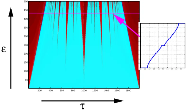
This kind of two-frequency behavior gives rise to a characteristic pattern, in the plane of ǫ vs. τ , called Arnol’d tongues. This pattern is computed numerically and shown in Fig. 9 for the family defined by (3.2), together with a section at a fixed value of ǫ. This cross-section exhibits the so-called Devil’s staircase, with “steps” on which the rotation number [53] is constant within each Arnol’d tongue; the rotation number measures the average rotation per iterate of (3.2).

For zero ǫ, two types of phenomena occur: either τ is rational and in this case the dynamics is periodic with period q, where τ = p/q, or τ is irrational and the iterates {xn}

fill the whole circle densely. As ǫ increases, an Arnol’d tongue of increasing width grows out of each τ = p/q on the abscissa ǫ = 0. It follows that, in this very simple case, such an Arnol’d tongue corresponds to hyperbolic dynamics that is robust to perturbations, as verified by linearizing the map at the periodic point; the rotation number is then rational and equal to p/q.

The set of all these tongues is dense within the whole circle map family, while the Lebesgue measure of this set, at given ǫ, tends to zero as ǫ goes to zero. On the contrary, if a point in the

(τ, ǫ)-plane does not belong to an Arnol’d tongue, the rotation number for those parameter values is irrational and the dynamics is nonhyperbolic; the latter fact follows, for instance, from a theorem of Denjoy [98] showing that such dynamics is smoothly equivalent to an irrational rotation. The probability to observe nonhyperbolic dynamics tends therewith to unity as ǫ goes to zero. One has, therefore, a countably infinite number of distinct topological classes, namely the Arnol’d tongues p/q, and an uncoutably infinite number of maps with irrational rotation numbers.

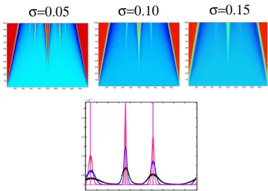
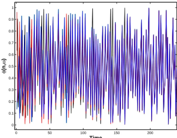
What happens when noise is added in Eq. (3.2)? We consider here the case of additive forcing by a noise process obtained via sampling at each iterate n a random variable with uniform density and intensity σ. Experiments with colored, rather than white noise and multiplicative, rather than additive noise led to the same qualitative results. The results for additive white noise are shown in Fig. 10 for three different levels of noise intensity σ.

As expected, only the largest tongues survive the presence of the noise; in particular, there is only a finite number of surviving tongues, shown in red in Fig. 10. Within such a surviving tongue, the random attractor A(ω) is a random periodic cycle of period q (not shown). In the blue region outside the Arnol’d tongues, the random attractor is a fixed but random point A(ω) = {a(ω)}: if one starts a numerical simulation for a fixed realization of the noise ω0, all initial data x converge to the same fixed point a0, say; see Fig. 11 in the

appendix.

This striking result tells us that noise destroys the irrational character of the dynamics; see the appendix: fractal structures, like the Devil’s staircase in Fig. 9, are likely to disappear in the presence of noise. Of course the generality and scope of such a conclusion need considerable further study, numerical as well as rigorously mathematical.

As shown in the lower panel of Fig. 10, there is also a direct relationship between the random dynamics and the support of the PDF on the circle. For a given noise level, this support can either be the union of a finite number of disjoint intervals (red and blue curves) or it can fill the whole circle (black curve). The random attractor is, accordingly, either a random periodic orbit, with the disjoint intervals being visited in succession, or a random fixed point; this PDF behavior characterizes the level of the noise needed to destroy a given tongue. An exact definition of random fixed point and random periodic orbit with period q is given in the appendix.

200 400 600 800 1000 1200 1400 1600 1800 50 100 150 200 250 300 350 400 450 500 0 0.10.2 0.30.4 0.50.6 0.70.8 0.9 0 0.1 0.2 0.3 0.4 0.5 0.6 0.7 0.8 0.9 1

ε

τ

Figure 9: Arnol’d tongues for the family of diffeomorphisms of the circle; units for τ and ǫ are 5 · 10−4_{and 10}−4_{respectively. Devil’s staircase in the cross-section to the right.}

frame-0 0.1 0.2 0.3 0.4 0.5 0.6 0.7 0.8 0.9 1 0 0.5 1 1.5 2 2.5 3 3.5 4 x 10−3

σ=0.10

σ=0.15

σ=0.05

Effect of the noise on the PDF of the Arnol’d tongue 1/3

Figure 10: Arnol’d tongues in the presence of additive noise with different noise amplitudes σ. Upper panels: Arnol’d tongues for σ = 0.05, 0.10 and 0.15; lower panel: PDF for ǫ = 0.9 and the three σ-values in the upper panels: σ = 0.05 (red curve), σ = 0.10 (blue curve), and σ = 0.15 (black curve).

work of RDS theory and rigorous studies on random circle maps. This theoretical analysis helps clarify the interaction between noise and nonlinear dynamics in the context of the classification problem we are interested in and it is provided in Appendix A.

4

Concluding remarks

We recall that Section 2 dealt with the natural, interannual and interdecadal variability of the ocean’s wind-driven circulation. The oceans’ internal variability is an important source of uncertainty in past-climate reconstructions and future-climate projections [8, 9, 10, 11]. In Section 3 and Appendix A, we dealt more generally with the problem of structural instability as a possible cause for the stubborn tendency of the range of uncertainties in climate change projections to increase, rather than diminish over the last three decades [1, 2, 3, 4]. We summarize here the main results of the two sections in succession, and outline several open problems.

The wind-driven double-gyre circulation dominates the near-surface flow in the oceans’ mid-latitude basins. Particular attention was paid to the North Atlantic and North Pa-cific, traversed by the best-known oceanic jets, namely the Gulf Stream and the Kuroshio Extension (see Fig. 2). The wind-driven circulation exhibits very rich internal dynamics and multiscale behavior associated with turbulent mesoscales (see Fig. 3). Aside from the intrinsic interest of this problem in physical oceanography, these major oceanic currents help regulate the climate of the adjacent continents, while their low-frequency variability affects past, present and furture global climate.

Thanks in part to the systematic use of dynamical systems theory, a comprehensive understanding of simple, barotropic, quasi-geostrophic (QG) models of the double-gyre cir-culation has been achieved over the last two decades, and was reviewed in Section 2 here. In particular, the importance of symmetry-breaking and homoclinic bifurcations (see Fig. 4)

in explaining the observed low-frequency variability has been validated across a wide hierar-chy of models, including models with much more comprehensive physical formulation, more realistic geometry, and greater resolution in the horizontal and vertical [10, 11].

The next challenge in physical oceanography, as well as in fluid mechanics in general, is to reconcile the points of view of dynamical systems theory and statistical mechanics in describing the interaction between the largest scales of motion and geostrophic mesoscale tur-bulence, which is fully captured in baroclinic QG models. We emphasize that the complexity of these models of the double-gyre circulation is intermediate between high-end GCMs and simple “toy” models; these models offer, therefore, an ideal laboratory to test our ideas. In particular, stochastic parametrizations of the rectification process, absent in barotropic QG models, could be studied using some of the concepts and tools from RDS theory presented here. Note that the RDS approach has already been used in the context of stochastic partial differential equations, in particular for showing the existence of random attractors, as well as stable, unstable and inertial manifolds. Thus RDS concepts and tools are not restricted to finite-dimensional systems [99, 100, 101].

In Section 3, we have addressed the range-of-uncertainty problem for IPCC-class GCM simulations (see Fig. 1) by considering them as stochastically perturbed dynamical systems. This approach is consonant with recent interest for stochastic parametrizations in the high-end modeling-and-simulation community [69, 70, 71, 72, 73, 74]. We have emphasized — based on rigorous mathematical results from the dynamical systems literature over the last few decades — that, in the absence of stochastic ingredients, GCMs as well as simpler models, on the lower rungs of the modeling hierarchy [26], are bound to differ from each other in their results.

This sensitivity follows from the fact that deterministic, hyperbolic systems — for which the stable and unstable manifolds are in general position, i.e. roughly speaking satisfy Axiom A plus strong transversality assumptions — are essentially the only structurally stable ones, at least in the C1_{case [57, 58, 59, 60]. Thus, because hyperbolic systems are not dense in the}

set of smooth deterministic ones [62], we are led to conclude that the topological, structural-stability approach does not guarantee deterministic-model robustness, in spite of its many valuable insights so far. Related issues for GCM modeling were emphasized recently by Held [81] and McWilliams [82] in a speculative mode.

We have proposed in this paper to go one step further, by considering the difficult question of model robustness in the presence of stochastic terms; such term could represent either parametrizations of unresolved processes in GCMs or stochastic components of natural or anthropogenic forcing, such as volcanic eruptions or fluctuations in greenhouse gas or aerosol emissions. Despite the obvious gap between idealized models and high-end simulations, we have addressed the problem here in the light of random dynamical systems (RDS) theory [16].

In this framework, we have considered a robustness criterion that could replace structural stability, through the concept of stochastic conjugacy (see Figs. 6 and 7). We have shown, for a stochastically perturbed Arnol’d family of circle maps, that noise can enhance model robustness. More precisely, this circle map family exhibits structurally stable, as well as structurally unstable behavior. When noise is added, the entire family exhibits stochastic structural stability, based on the stochastic-conjugacy concept, even in those regions of parameter space where deterministic structural instability occurs for vanishing noise (see Figs. 9 and 10).

Clearly the hope that noise can smooth the very highly structured pattern of distinct behavior types for climate models, across the full hierarchy, has to be tempered by a number of caveats. First, serious questions remain at the fundamental, mathematical level about the behavior of nonhyperbolic chaotic attractors in the presence of noise [84, 85, 86]. Likewise,