HAL Id: hal-01626468
https://hal.archives-ouvertes.fr/hal-01626468
Submitted on 26 Nov 2020
HAL is a multi-disciplinary open access
archive for the deposit and dissemination of
sci-entific research documents, whether they are
pub-lished or not. The documents may come from
teaching and research institutions in France or
abroad, or from public or private research centers.
L’archive ouverte pluridisciplinaire HAL, est
destinée au dépôt et à la diffusion de documents
scientifiques de niveau recherche, publiés ou non,
émanant des établissements d’enseignement et de
recherche français ou étrangers, des laboratoires
publics ou privés.
Distributed coordination model for smart sensing
applications
Luca Maggiani, Lobna Ben Khelifa, Jean-Charles Quinton, Matteo Petracca,
Paolo Pagano, François Berry
To cite this version:
Luca Maggiani, Lobna Ben Khelifa, Jean-Charles Quinton, Matteo Petracca, Paolo Pagano, et al..
Distributed coordination model for smart sensing applications. 10th International Conference on
Dis-tributed Smart Camera (ICDSC ’16), Sep 2016, Paris, France. pp.110-115, �10.1145/2967413.2967438�.
�hal-01626468�
Distributed coordination model for smart sensing
applications
Luca Maggiani
∗Scuola Superiore Sant’Anna Pisa, Italy
Lobna Ben Khelifa
Clermont University / CNRS Clermont-Ferrand, France
Jean-Charles Quinton
Grenoble Alpes Univ. / CNRS Grenoble, France
Matteo Petracca
Scuola Superiore Sant’Anna Pisa, Italy
Paolo Pagano
CNIT, National Laboratory of Photonic Networks Pisa, Italy
François Berry
Clermont University / CNRS Clermont-Ferrand, FranceABSTRACT
Distributed networks of smart sensors are nowadays rep-resenting the frontier of Machine-to-Machine (M2M) inter-operability. In such a scenario several challenges must be addressed in order to create effective solutions. Coordina-tion among nodes to satisfy monitoring purposes while ad-dressing network constraints is considered of utmost impor-tance. In this respect, the paper proposes a novel coordi-nation model for self-organizing smart monitoring systems. The proposed algorithm is able to autonomously retrieve event correlations from the environment in order to coordi-nate the nodes. By relying on temporal and spatial corre-lations, the proposed system can be particularly suited for Smart Camera Network (SCN) deployments where multiple cameras monitor distributed targets. Along the algorithm definition, the paper presents a performance evaluation of the proposed approach through simulations, thus evaluating the robustness of the proposed model against message losses.
1.
INTRODUCTION
With nowadays improvements in information and com-munications technologies, more and more sensors are de-ployed to monitor our daily life. Traffic control sensors, ac-cess authentication systems and environmental monitoring are already widespread within our cities [1, 2]. Moreover, by overtaking the limits of a classical centralized control, sensor networks are evolving towards complete Cyber-Physical Sys-tems (CPSs), where sensing, processing and communication policies are distributed over the network nodes. The con-struction, processing and transfer of semantic information can then be achieved through node-to-node communication, ∗email: [email protected]
Permission to make digital or hard copies of all or part of this work for personal or classroom use is granted without fee provided that copies are not made or distributed for profit or commercial advantage and that copies bear this notice and the full cita-tion on the first page. Copyrights for components of this work owned by others than ACM must be honored. Abstracting with credit is permitted. To copy otherwise, or re-publish, to post on servers or to redistribute to lists, requires prior specific permission and/or a fee. Request permissions from [email protected].
ICDSC ’16, September 12-15, 2016, Paris, France
c
2016 ACM. ISBN 978-1-4503-4786-0/16/09. . . $15.00
DOI:http://dx.doi.org/10.1145/2967413.2967438
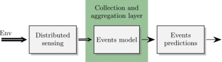
thus following the M2M interaction model. At a higher level, computing architectures are moving away from centralized and static deployment to autonomous entities distributed in the environment. As introduced in [3], distributed comput-ing is challengcomput-ing the computer science academia to describe and understand novel and more complex models of interac-tions [4]. Indeed, in designing distributed systems – and in system of systems applications as well [5] – a multi-layer formalization is needed. In this respect, we refer to the three layers shown in Fig. 1. Since in the environment a dis-tributed sensing is performed by each sensor autonomously, a cloud of local measures – called events – is then generated. These local events are eventually analyzed and classified to recover higher level events according to a system model. The event model can be seen as a correlation map of the environ-ment, based on the measured observations. This represents the cornerstone for higher level data aggregations and the main target of this paper. Once the model has been defined, each local event can be classified by inferring from correla-tions with its neighbor events, thus enabling event prediction properties.
Distributed
sensing Events model Env
Collection and aggregation layer
Events predictions
Figure 1: A distributed sensing environment formalization. As long as the network remains relatively small, the event model can be statically defined as a function of the node calibrations. Consider a Smart City scenario where a set of Smart Cameras (SCs) trigger events in response to ve-hicles movements, and witness a road accident. Based on cameras placement, the event semantics can be empirically estimated due to the well-constrained scenario (e.g., vehicles directions, speed). However, along with the network growth or in case of variability (e.g., roundabout, pedestrian move-ments), retrieving the semantics and relationships between nodes will rapidly become more complex. Moreover, due to the often noisy input and detection glitches (false alarms),
a single sensor measure alone might not be reliable enough to guarantee correct higher level inferences.
Nonetheless, not all interactions are equally important: weighted connections between nodes are indeed common-place in network based real-world problems. The concept of weighted connection topologies is a well-known method to model connection patterns for autonomous agent-based networks. In particular, in [6] the concept has been ap-plied to characterise latent brain activities during functional Magnetic Resonance Imaging (fMRI). This led the authors to a Markov-based linear model – called Dynamic Causal Model (DCM) – to analyse and evaluate the connectivity based on observed neuronal responses. The same principle can be found in [7], where a weighted Markov chain is de-ployed to predict the spreading process of epidemic disease. Closer to the communication network domain, notable ap-plications are the Page Rank algorithm by Google [8] and the consensus and averaging algorithms as in [9]. The for-mer evaluates the web page importance as the capability to connect other high quality nodes in its surrounding. The lat-ter represents instead a state-of-the-art proposal for SCNs, where a combination of measures and distributed agreement algorithms are deployed to enforce the consensus forma-tion [10–14].
Our proposed distributed coordination model addresses the aforementioned issues by leveraging self-organizing node interactions. These interactions are used to: (i) make the system adapt to changing environment conditions and to unpredicted events, (ii) improve the detection reliability by aggregating conform events, (iii) improve the system robust-ness against node malfunction [9] and detection glitches. The proposed distributed coordination model is inserted into the collection and aggregation layer, as in the middle step in Fig. 1. In other words, we made the assumption that the distributed system – e.g., a SCN – is able to generate higher level events from collected local measures. These measures are then collected and semantically aggregated by the Event model which formally defines the interaction patterns. The model produces the most-probable node interactions, ac-cording to spatial and temporal correlations mesured be-tween nodes.
The remainder of the paper is organized as follows. The mathematical notations and the system description are pre-sented in the next section. In Section 3 the proposed model is presented. Section 4 shows the evaluation results. Finally, the conclusion is drawn and future directions are described in Section 5.
2.
SYSTEM DESCRIPTION
In the considered scenario measures are autonomously performed by each node over its well-behaved local sur-roundings. The system environment results then in a man-ifold space composed by aggregating overlapped local mea-surement spaces. Each node is defined with the identifier Cn and its relative state sn. The state sn represents the
node rank within the network and its contribution to the distributed coordination. The node state vector at time k is defined as:
sk= {s1, . . . , sN}k (1)
where N is the number of nodes at time k. Moreover, each node describes its surroundings by defining a visibility range, namely the maximum distance within the target is detected
by the node itself. On first approximation omnidirectional visibility spaces and uniform detection ranges are consid-ered. This limit is initially introduced to simplify the math-ematical formalism where further investigations are consid-ered as future perspectives. The targets are moving entities
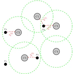
C2 C5 C3 C1 C4 x1 x2 x3 x4 z(1)2 z(3)2 z3(5) z(2)4
Figure 2: An instance of the system environment space, with visibility ranges as dashed circles.
which are defined by their signatures, e.g., visual features, positions, speeds, trajectories. The target vector is defined as:
xk= {x1, . . . , xM}k (2)
where each component represents a target signature and M the number of targets that appear at time k. The causal evolution of xkis described as:
x0= Gk(xk) (3) where Gk(·) is a Markov chain process of the vector xk and x0 represents the target at interval k + 1. In particular, Gk
is a memory-less stochastic process with unobservable states (as known as Markov assumption). As a consequence, the behaviour of the xm with m ∈ M target at time k can
be evaluated as the probability distribution of the previous k − 1 sample rather than the complete set of the target sam-ples x = {xk−1, xk−2, . . . }.
The targets are observed by the nodes through measures (if targets reside in the visibility range). Each measure is an approximation of the target features with respect to a specific node at one specific time interval. The observation vector is therefore defined as follows:
zk= {z1, . . . , zM}k (4)
where M still considers the available targets at time k. Since each node performs its own measures, multiple appearances of xk could exist. In particular, from the node C1 the ob-servation vector is defined as:
z(1,k)= {z11, . . . , z 1 M}
k
as seen from C1 (5) For instance, in Fig. 2 a system environment space is de-picted. Here five nodes are instantiated C1, · · · , C5 with
their states s1, · · · , s5 respectively. With this respect,
tar-gets x1, · · · , x4are arbitrarily placed and are moving
follow-ing a deterministic trajectory. The z(2)4 measure refers to
the x4target being detected inside the visibility area of C2.
Since x2 belongs to the C3 and C1 visibility areas, double
target measures are then retrieved. Due to the noisy envi-ronment and to the different spatial conditions, these mea-sures are only ideally equivalents while they present some degrees of correlation. The distributed coordination model, which is the main contribution of this paper, is then defined as:
s0= Fk(sk, zk) (6) where Fk(·) represents the state transition function. The state vector s0 at time sample k + 1 becomes then a func-tion of the previous state vector sk and of the performed measures zk. Through local observations, the aim of the coordination is to reinforce the nodes interactions by ap-proximating the Gk function with the a-posteriori
evalua-tion Fk. In the next section, the structure of Fkis analysed by proposing a novel methodology.
3.
DISTRIBUTED NETWORK MODEL
According to the Eq. 6, our discrete time model is for-malized as a function of it previous state sk and the input stimuli vector applied to the system zk. Assuming a bi-linear Taylor transformation of F , in Eq. 7 the dependencies in s and z are expressed.
ds dt = ∂F ∂s|zds + ∂F ∂z|sdz + ∂2F ∂s∂zdsdz (7) where A = ∂f ∂s|z and B = ∂f ∂z|s and C = ∂A ∂zdz (8) Finally, in Eq. 9 the system model equations are expressed. The vector notation is derived from the Eq. 6 and makes it suitable to multiple node instances. The scalar values A, B, C as in Eq. 7 become square matrices A, B, C and s0 the state vector s0. The Eq. 9 also expresses the temporal dependence of the A0term as the combination of the A and C of the previous iteration.
s0= As + Bz
A0= A + C (9) The system dynamic s0is driven by the input measures z in two separate contributions: (i) the response to direct stimuli through B matrix or (ii) the induced interactions according to the C matrix (as Eq. 8). The A matrix results from the Bayes assumption, where the next state depends on the a-posteriori probability of interaction. The matrix B instead represents observation space and the source term in the sys-tem. Finally, the dynamic and time-changing term C adds to the state matrix the induced connectivity as results of interaction pattern in the environment (it creates/removes connections coupling). In the following, the A, B, C contri-butions are considered to evaluate their effect on the state transition function Fk.
3.1
Stochastic connectivity
According to Eq. 9, the A matrix represents the next-state transition probability from the vector state s. This is mod-eled as a stochastic adjacency matrix and contains N × N
non-negative entries for every possible state transition. For a given state snrelated to the n − th node, the interactions
with the others can be expressed as a linear combination of the row elements of A. These interactions are described as unidirected graphs, where connections are expressed as edges and nodes as vertex. The existence of interaction is revealed by a non-zero probability pij between the source
node i and the target node j. c1 c2 c3 c4 c5 p21 p23 p13 p34 p45 p54
Figure 3: A connectivity graph example based on Fig. 2. For instance, assume that Fig. 3 represents the connectiv-ity graph of the system in Fig. 2. A connection exists from C3 towards C4 but no interaction is defined between C2 and C5 though. The existence of an interaction is due to the pre-vious measured activities (e.g., events correlation) between nodes. This concept, borrowed from the biology [15] and social network [16] studies, allows to represent distributed networks as functional connectivity between entities. An ac-tive communication is therefore defined by A as a probabil-ity distribution and it is not related to the physical network topology – e.g., Received Signal Strength Indicator (RSSI). For instance, far apart nodes with low RSSI unlikely mea-sures correlated events unless considering complex environ-ment configuration. On the other side, nodes with high signal strengths might not automatically showing correla-tion between their measures. Thus, signal structure features can not be used to assess event correlations but they might rather considered as a complementary information to the model.
According to Eq. 9, A is a right stochastic matrix, with each row summing to 1. This property induces that the state transitions are balanced between the outgoing transitions (pijwith i 6= j) and the steady state pii one. The lower pii,
the higher is the importance of interactions. This results in a trade-off between steady state and transitions which depends on the importance given to communications rather than on the measures available in the node itself. In Eq. 10 the network connections shown in Fig. 3 are described.
A = p11 0 p13 0 0 p21 p22 p23 0 0 0 0 p33 p34 0 0 0 0 p44 p45 0 0 0 p54 p55 (10)
At system initialization, the relevant communication pat-terns between nodes is not usually known. The stochas-tic matrix A is therefore initialized to uniformly distributed probabilities. This means that each interaction is equally important and any distinction between them is to be later
inferred. Thus, according to the Eq. 9 and in absence of the source term, the system is in a steady state (the state vector s is null). Through observations relevant correlations are collected and used to update the stochastic model of A. This event gathering phase (as in Fig. 1) is an on-line process that continuously measures and adapts the system response towards the likelihood expectation.
3.2
Observation matrix
While temporal event correlation drives the stochastic and the induced connectivity matrices, the spatial correlations are considered for measures. According to Eq. 11, the ob-servation matrix B represents the obob-servation space, as com-posed by the multiple measures of the target vector z per-formed by the N nodes.
B = {znm} k
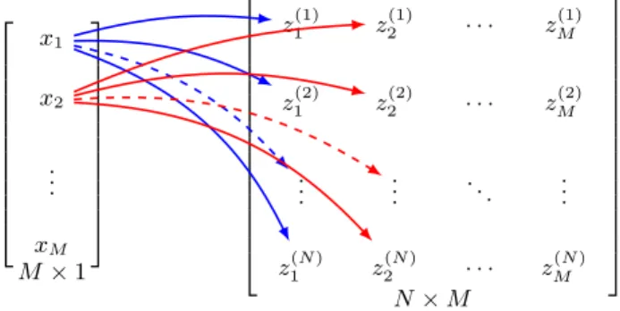
n ∈ {1, N }, m ∈ {1, M } (11) In Fig. 4 the relationship between the observation matrix and the target vectors is shown. Since physical systems are unlikely fully observable, the B is considered as a sparse matrix. A zeroed column i means that the target xi is not
visible from the system therefore the relative measures are not considered. Each element of B represents how much two
x1 x2 . . . xM z(1)1 z2(1) · · · z(1)M z(2)1 z (2) 2 · · · z (2) M . . . ... . .. ... z(N )1 z2(N ) · · · z(N )M N × M M × 1
Figure 4: The relationship between the target vector x and the observation matrix B.
measures are correlated within the same temporal interval k. This usually results in a geometrical evaluation between visibility ranges. The way of deriving it actually depends on the physical phenomenon under measure. For instance, in SCNs the spatial correlations are related the cameras’ field of views intersections and can be evaluated using affine region detectors [17] or the Simultaneous Localization And Map-ping (SLAM) technique [18]. For proprioceptive sensors, e.g. vibration, temperature, spatial correlation is rather evalu-ated with correlation indexes, such as Moran’s I [19].
3.3
Induced connectivity
Given a set of events occurred within the network, nodes that are showing relevant event correlations are establishing active communications among them. Each node is mod-eled as an autonomous agent which tries to learn the opti-mal neighbor selection policy from its history of interaction. Since the environment has been defined as a Markov pro-cess (according to Gk), events correlations are meaningful
information to reveal repetitive patterns of behaviour. In Eq. 12, a simplified version of the Q-Learning algorithm [20] has been used to evaluate the induced connectivity as the C term.
C = α(R − A) (12)
where α ∈ R[0, 1) is the learning rate, R is the reward ob-served after validating the prediction. The elements of C can be computed as follows:
cij= α(rij− pij) (13)
where pijis the likelihood that the event (measure of a
tar-get) evolves from the camera i to the camera j (see Eq. 10). The reward term rij is related to the temporal correlation
analysis between available measures from camera i to j. This factor is evaluated using a Gaussian probability distribution Nij(τm,ij, σ2ij) centred at the delay time expectation τm,ij
between nodes. For instance, if a target x1is detected from
the node C1 and then from the node C2, the delay time as τ12 can be measured. If this target is periodically
de-tected between the nodes, an expected delay time τm,12can
be also estimated. Since then, in order to evaluate whether nodes are temporally correlated or not, the measured τ12
is compared to the τm,12 through the time delay
distribu-tion. The closer is τ12to the model average, the higher
cor-relation probability results. Then higher corcor-relation turns to higher r12 reward. By iteratively updating the τm
av-erages and giving the likelihood probability of correlation, the nodes strengthen their coordination in case of correlated event and vice versa. In Eq. 14 the reward rijcomputation
is expressed as function of the standard deviation σij.
rij= +1 if τij− τm,ij≤ σij −1 if τij− τm,ij≥ 2σij 0 else (14)
Since the probability distributions Nijare on-line computed,
the reward evaluations are continuously updated to meet en-vironmental variations and to detect abnormal events that might occur. The third case in Eq. 14, which brings a neu-tral reward, has been introduced as an hysteresis guard that prevents reward oscillations.
4.
EVALUATION
In this section, a simple smart sensing application is con-sidered to evaluate the methodology presented in Section 3. In the proposed evaluations, we show how the system is autonomously coordinating the nodes interactions as results of specific event patterns. The system is composed of a set of nodes which are able to perform measurements whitin their own visibility range and to communicate with others. For instance, this would be the case of a distributed video-surveillance deployment, where each node is a SC able to detect visual targets. No knowledge about node positions, visibility ranges and neighborhoods are needed during sys-tem setup.
The simulations are performed using the discrete event simulator OMNeT++ [21], installed in a PC workstation. The main goal of these preliminary evaluations is to show the effect of nodes coordination to reach a stable state with-out assumptions on the setup environment. Moreover, the system is also evaluated in term of robustness with respect to message losses (as an uniform density of probability of los-ing messages) and to glitches detection (which causes false alarms).
The state transition probabilities pijare initially setup to
1/N (where N is the number of the available nodes, as in Eq. 1). Assuming this uniform probability results in an ini-tially unbiased state transition policy. Moreover, the target
C1 p12 C2 p23 C3 p34 C4 x1
Figure 5: Aligned nodes configuration.
trajectories are deterministic with constant motion speeds and the observation matrix B is considered equivalent to an identity matrix. In the followings, the state transition probability is then computed according to Eq. 13 as:
p0ij= pij+ α(rij− pij) (15)
where α is fixed to 0.2 and the reward is computed as in Eq. 14. The expected delays time τm,ij are evaluated as
a weighted moving average over the last measures by each node in order to reduce the effect of outliers.
4.1
Aligned nodes
In Fig. 5 the first setup configuration is shown. In par-ticular, the nodes C1, · · · , C4 are aligned to the target x1
trajectory. The target is repeatedly following the same path, from the left to the right side (the dashed line in Fig. 5).
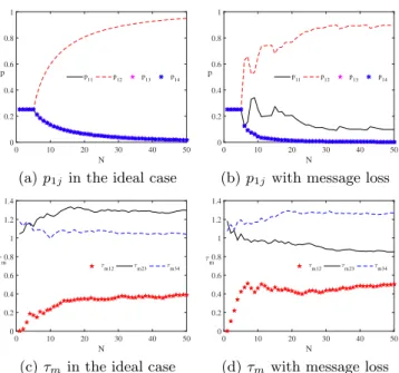
In Fig. 6 the simulation results are shown for 50 time sam-ples. In particular, in Fig. (a) the state transition probabili-ties p1jfrom node C1 are computed. The p1j are computed
according to Eq. 9 and initially setup to 1/4. After the start-up phase, the p12 probability increases while p13, p14
decrease. Also p11decreases as well as p12converges towards
1. In Fig. (b), the expected time τmijare shown. These time
references are continuously updated with new measures. As expected, as long as the system converges towards stable transition probabilities, the τm indexes are stable as well.
In Fig. 6c and 6d the same system configuration is evalu-ated in case of random communication failures. Although the target is still following the same trajectory, the system response is slower than in the ideal case but yet reaches a sta-ble state. It worth noting that the fluctuation of p12due to
the communication noise are absorbed by the steady state s11 through p11. This means that if the node experiences
message losses, its state transition probability decreases in favor of the steady state probability.
4.2
Non-aligned nodes
The second configuration introduces nodes C1, · · · , C4 with a non aligned configuration. In this case, also the target x1
trajectory might change between the two dashed lines in Fig. 7. Once again, the evaluation is presented in the Fig. 8 as function of the stochastic connectivity and the expected delay time τmseen from the node C2. With respect to the
other case, the environment presents more variability thus resulting in more unstable behaviour. Therefore the simula-tion in the ideal case and in case of message loss are extended to 100 and 1000 time samples respectively. Since the trajec-tory path is randomly chosen between the two available, in Fig. 8a both p23 and p24 are varying accordingly with
the current path. These transition probabilities asymptoti-cally converges to the decision rate between trajectories. For these simulations a uniform probability rate has been used, thus both p23and p24asymptotically reaches 0.5. Although
the trajectories are randomly chosen, the target movements are still deterministic. This explains the relative stability
N 0 10 20 30 40 50 p 0 0.2 0.4 0.6 0.8 1 p 11 p12 p13 p14
(a) p1j in the ideal case
N 0 10 20 30 40 50 p 0 0.2 0.4 0.6 0.8 1 p 11 p12 p13 p14
(b) p1jwith message loss
N 0 10 20 30 40 50 τ m 0 0.2 0.4 0.6 0.8 1 1.2 1.4 τm12 τm23 τm34
(c) τmin the ideal case
N 0 10 20 30 40 50 τ m 0 0.2 0.4 0.6 0.8 1 1.2 1.4 τm12 τm23 τm34
(d) τm with message loss
Figure 6: The system dynamic seen from node C1 in the aligned nodes setup.
C3 C2 C4 C1 x1 x1 p12 p23 p24
Figure 7: Non-aligned nodes configuration.
of the time delay expectations τm in Fig. 8b with respect
to the state transition rates. As long as the environment presents event correlation patterns, the system is able to ex-tract stable time delay expectations. In Fig. 8c the message loss impact are shown for the non aligned configuration. As expected, the steady state probability p22 is absorbing the
system fluctuation by reducing the state transition rate. As a result, the system takes more time to converge (the time scale has been extended to 1000 samples) as previously seen in Fig. 6c. No qualitative variations are instead evaluated in Fig. 8d with respect to the ideal case in Fig. 8b.
5.
CONCLUSIONS
In the paper a novel distributed coordination model for smart sensing application has been proposed. The presented methodology is suitable for autonomous smart sensing ap-plication, where the nodes are arbitrarily placed in the en-vironment. With respect to standard sensor deployments, a coordination algorithm simplify the system installation and reduces the maintenance. The preliminary evaluations pro-posed in this paper shows robustness with respect to message losses or detection glitches.
Many are the future perspectives. First of all, we will fur-ther simulate the model with more complex networks with different experimental conditions. Then the algorithm will
N 0 20 40 60 80 100 p 0 0.2 0.4 0.6 0.8 1 p 23 p24 p21 p22
(a) p2j in the ideal case
N 0 200 400 600 800 1000 1200 p 0 0.2 0.4 0.6 0.8 1 p 23 p24 p21 p22
(b) p2j with message loss
N 0 20 40 60 80 100 τ m 0.6 0.7 0.8 0.9 1 1.1 1.2 1.3 1.4 τm12 τm23 τm24
(c) τmin the ideal case
N 0 200 400 600 800 1000 1200 τ m 0.6 0.7 0.8 0.9 1 1.1 1.2 1.3 1.4 τm12 τm23 τm24
(d) τmwith message loss
Figure 8: The system dynamic seen from node C2 in the non-aligned nodes setup.
be evaluated in a physical SCN scenario, where node coor-dination can be used as a distributed target tracking appli-cation.
Acknowledgment
This work has been partially sponsored by the French gov-ernment research program “Investissements d’avenir” through the IMobS3 Laboratory of Excellence and by the the Eu-ropean Union under the EuEu-ropean Regional Development Fund (ERDF).
6.
REFERENCES
[1] Daniele Miorandi, Sabrina Sicari, Francesco De Pellegrini, and Imrich Chlamtac, “Internet of things: Vision, applications and research challenges,” Ad Hoc Networks, vol. 10, no. 7, pp. 1497 – 1516, 2012. [2] Charith Perera, Chi Harold Liu, Srimal Jayawardena,
and Min Chen, “A survey on internet of things from industrial market perspective,” IEEE Access, vol. 2, pp. 1660–1679, 2014.
[3] Dan Chalmers, Matthew Chalmers, Jon Crowcroft, Marta Kwiatkowska, Robin Milner, Eamonn O’Neill, Tom Rodden, Vladimiro Sassone, and Morris Sloman, “Ubiquitous computing: experience, design and
science,” in Ubiquitous Computing: 8th International Conference, 2006.
[4] Morris Sloman, Martyn Thomas, Karen Sparck-Jones, Jon Crowcroft, Marta Kwiatkowska, Paul Garner, Nicholas R Jennings, Vladimiro Sassone, Eamonn O’Neill, Michael Wooldridge, et al., “Discussion on robin milner’s first computer journal lecture: ubiquitous computing: shall we understand it?,” The Computer Journal, 2006.
[5] Dominik Wachholder and Chris Stary, “Enabling emergent behavior in systems-of-systems through bigraph-based modeling,” in System of Systems
Engineering Conference (SoSE), 2015 10th. IEEE, 2015, pp. 334–339.
[6] Karl J Friston, Joshua Kahan, Bharat Biswal, and Adeel Razi, “A dcm for resting state fmri,” Neuroimage, vol. 94, pp. 396–407, 2014.
[7] Eugenio Valdano, Luca Ferreri, Chiara Poletto, and Vittoria Colizza, “Analytical computation of the epidemic threshold on temporal networks,” Physical Review X, vol. 5, no. 2, pp. 021005, 2015.
[8] Lawrence Page, Sergey Brin, Rajeev Motwani, and Terry Winograd, “The pagerank citation ranking: bringing order to the web.,” 1999.
[9] Reza Olfati-Saber, J Alex Fax, and Richard M Murray, “Consensus and cooperation in networked multi-agent systems,” Proceedings of the IEEE, vol. 95, no. 1, pp. 215–233, 2007.
[10] Uˆgur Murat Erdem and Stan Sclaroff, “Event prediction in a hybrid camera network,” ACM Trans. Sen. Netw., vol. 8, no. 2, pp. 16:1–16:27, Mar. 2012. [11] Dragana Bajovic, Joao Xavier, Jos´e MF Moura, and
Bruno Sinopoli, “Consensus and products of random stochastic matrices: Exact rate for convergence in probability,” Signal Processing, IEEE Transactions on, vol. 61, no. 10, pp. 2557–2571, 2013.
[12] Prabhu Natarajan, Pradeep K Atrey, and Mohan Kankanhalli, “Multi-camera coordination and control in surveillance systems: a survey,” ACM Transactions on Multimedia Computing, Communications, and Applications (TOMM), vol. 11, no. 4, pp. 57, 2015. [13] Aiping Wang, “Event-based consensus control for
single-integrator networks with communication time delays,” Neurocomputing, 2016.
[14] Guillem Mart´ınez-C´anovas, Elena Del Val, Vicente Botti, Pen´elope Hern´andez, and Miguel Rebollo, “A formal model based on game theory for the analysis of cooperation in distributed service discovery,”
Information Sciences, vol. 326, pp. 59–70, 2016. [15] Klaas Enno Stephan and Karl J Friston, “Models of
effective connectivity in neural systems,” in Handbook of Brain Connectivity, pp. 303–327. Springer, 2007. [16] Mehmet C Vuran, ¨Ozg¨ur B Akan, and Ian F Akyildiz,
“Spatio-temporal correlation: theory and applications for wireless sensor networks,” Computer Networks, vol. 45, no. 3, pp. 245–259, 2004.
[17] Krystian Mikolajczyk, Tinne Tuytelaars, Cordelia Schmid, Andrew Zisserman, Jiri Matas, Frederik Schaffalitzky, Timor Kadir, and Luc Van Gool, “A comparison of affine region detectors,” International journal of computer vision, vol. 65, pp. 43–72, 2005. [18] Randall Smith, Matthew Self, and Peter Cheeseman,
“Estimating uncertain spatial relationships in robotics,” in Autonomous robot vehicles, pp. 167–193. Springer, 1990.
[19] Patrick AP Moran, “Notes on continuous stochastic phenomena,” Biometrika, vol. 37, no. 1, pp. 17–23, 1950.
[20] Christopher John Cornish Hellaby Watkins, Learning from delayed rewards, Ph.D. thesis, University of Cambridge England, 1989.
[21] Andr´as Varga, “Omnet++ discrete event simulation system,” 2008.