HAL Id: hal-02168804
https://hal.archives-ouvertes.fr/hal-02168804
Submitted on 11 May 2020
HAL is a multi-disciplinary open access
archive for the deposit and dissemination of
sci-entific research documents, whether they are
pub-lished or not. The documents may come from
teaching and research institutions in France or
abroad, or from public or private research centers.
L’archive ouverte pluridisciplinaire HAL, est
destinée au dépôt et à la diffusion de documents
scientifiques de niveau recherche, publiés ou non,
émanant des établissements d’enseignement et de
recherche français ou étrangers, des laboratoires
publics ou privés.
microscopy
Laurent Moreaux, Olivier Sandre, Jerome Mertz
To cite this version:
Laurent Moreaux, Olivier Sandre, Jerome Mertz. Membrane imaging by second-harmonic generation
microscopy. Journal of the Optical Society of America B, Optical Society of America, 2000, 17 (10),
pp.1685. �10.1364/JOSAB.17.001685�. �hal-02168804�
Membrane imaging by second-harmonic
generation microscopy
L. Moreaux
Laboratoire de Neurophysiologie, Ecole Supe´rieure de Physique et Chimie Industrielles, Institut National de la Sante´ et de la Recherche Me´dicale EP00-02, 10 rue Vauquelin, 75005 Paris, France
O. Sandre
Laboratoire Physico-Chimie, Institut Curie, Centre National de la Recherche Scientifique, Unite´ Mixte de Recherche 168, 11 rue Pierre et Marie Curie, 75005 Paris, France
J. Mertz
Laboratoire de Neurophysiologie, Ecole Supe´rieure de Physique et Chimie Industrielles, Institut National de la Sante´ et de la Recherche Me´dicale EP00-02, 10 rue Vauquelin, 75005 Paris, France
Received February 24, 2000; revised manuscript received May 22, 2000
We present a detailed analysis of the generation of second-harmonic radiation from biological membranes la-beled with a styryl dye. In particular, we consider the numerical-aperture limit appropriate to high-resolution microscopy in which an excitation beam is tightly focused from the side onto a membrane surface. In this limit the active surface area that contributes to second-harmonic generation (SHG) depends only on the tightness of the beam focus and the SHG radiation is confined by phase matching into two well-defined off-axis lobes. We derive expressions for the SHG radiation power, angular distribution, and polarization dependence in the cases of ideal or nonideal molecular alignment in the membrane and uniaxiality of the molecular hy-perpolarizability. We define an SHG cross section similar to that used in two-photon-excited fluorescence (TPEF) to permit direct comparison of the two imaging modalities. Finally, we corroborate our results with experiments based on the excitation of a styryl dye in giant unilamellar vesicles with a mode-locked Ti:sap-phire laser.
OCIS codes: 190.416, 190.4180, 180.5810, 190.4350, 190.4710.
1. INTRODUCTION
Nonlinear optics is proving to be a powerful tool for bio-logical imaging. Fluorescence microscopy by two-photon excitation1–3 has become a laboratory standard, and three-photon excitation has demonstrated its feasibility.4,5 More recently, nonlinear microscopies based on radiative harmonic generation have also been applied to the imaging of surfaces6,7 and biological samples. Second-harmonic generation (SHG) has been used to image the intrinsic nonlinear susceptibility of muscle tissues8 and to image living cells labeled with styryl dyes.9,10 Third-harmonic generation has also been
used to provide microscopic images of cells and plant samples.11,12 Harmonic generation is an optical
phenom-enon involving coherent radiative scattering, whereas fluorescence generation involves incoherent radiative ab-sorption and reemission. As such, fluorescence and har-monic images are derived from fundamentally different contrast mechanisms. Moreover, because of its coherent nature, harmonic radiation is usually highly directional and depends critically on the spatial extent of the emis-sion source, making a full description of harmonic genera-tion more complicated than fluorescence generagenera-tion. We limit our discussions here to the description of molecular SHG only, with the understanding that many of our tech-niques may be generalized to higher-order harmonics.
It is well known that SHG of dipolar origin cannot arise from a medium that possesses an inversion symmetry. Therefore molecular SHG is usually studied in geometries in which the radiating molecules are spatially ordered. A common geometry is that of a planar interface or a sur-face that imparts a preferential orientation to a thin layer of molecules.13 Typically, the layer is illuminated at an oblique angle by a laser beam, resulting in the emission of SHG beams in well-defined reflection and transmission directions.14,15 Because the laser beam is usually unfo-cused or weakly founfo-cused, both the driving laser field and the resultant SHG fields can be treated as simple colli-mated beams with well-defined wave vectors, and the layer of molecules is most appropriately described in this geometry by a macroscopic surface susceptibility that is independent of the illuminated surface area.
In contrast, if SHG is intended to provide microscopic image resolution, the driving laser beam must be focused to a small spot size. The driving field can no longer be considered a simple plane wave as above, and the struc-ture of the resultant SHG radiation becomes critically de-pendent on the particular geometry of the driving field near the focal center. The use of a macroscopic surface susceptibility to quantify the SHG emission becomes in-appropriate in this case, and one must resort to a more refined description of the surface nonlinearity for length
scales much smaller than the radiation wavelength. In particular, it becomes necessary to redefine a surface non-linearity starting from the level of individual molecular hyperpolarizabilities (or nonlinear molecular cross sec-tions).
In this paper we provide a detailed theoretical descrip-tion of SHG emission appropriate to a high-resoludescrip-tion scanning microscope configuration that uses a tightly fo-cused excitation beam. The sensitivity of SHG emission to tight focusing has already been recognized for bulk nonlinear crystals.16 Because our attention is directed to biological imaging we consider here the different geom-etry of molecular SHG from membrane surfaces, as has been demonstrated experimentally in the imaging of cells and vesicles.10,17,18 We begin by characterizing the SHG emission from a single hyperpolarizable molecule in terms of a nonlinear scattering cross section. We then extend our discussion to the characterization of SHG emission from a planar distribution of molecules. In par-ticular, we adopt a formalism that specifically permits a direct comparison between the radiated powers in the case of SHG and in the corresponding case of two-photon-excited fluorescence (TPEF); the latter is already well es-tablished in biological microscopy. Indeed, recent results show that simultaneous SHG and TPEF can be obtained from the same collections of molecules. Finally we cor-roborate our theoretical formalism with experiments based on a full characterization, in terms of power, angu-lar distribution, and poangu-larization, of the SHG radiation obtained from giant unilamellar vesicles labeled with styryl dye. Our research here serves as a follow-up to provide complete theoretical and experimental support for the results presented in Ref. 18.
2. THEORY OF SHG MICROSCOPY
A. Single Molecule
We begin by defining the SHG cross section of a single molecule. The most straightforward definition entails calculating the total radiated SHG power and dividing this by the square of the incident driving field intensity. In particular, a molecule is considered an elemental di-pole radiator driven by the excitation light according to its first hyperpolarizability. For simplicity we assume that the excitation field is linearly polarized in the zˆ di-rection and begin by examining only the zzz component
of this hyperpolarizability, denoted . If the excitation light has frequency, the induced dipole moment at fre-quency 2 will be given by
2⫽1/2E2zˆ, (1)
where E is the excitation field amplitude and we have
used the Taylor convention.19 The radiated second-harmonic far field at an inclination from the z axis is
E2共兲 ⫽ ⫺
22
0c2r
sin共兲exp共⫺2i关t兴兲ˆ, (2) where 0 is the free-space permittivity, c is the speed of
light, r is the observation distance from the dipole, and [t] is the corresponding retarded time. The resultant power
per differential solid angle at an inclination, in units of photons/second, may be expressed as
P2共兲 ⫽ 163 SHGsin2共兲I2, (3)
where I is the excitation intensity in units of (photons/
second)/area and SHG⫽
4n2ប5
3n203c5
兩兩2 (4)
(nand n2are the indices of refraction at and 2; ប is Planck’s constant). We have definedSHGsuch that the
total SHG power, obtained by integration of Eq. (3) over all solid angles, reduces to the simple expression
PSHG⫽ 1/2SHGI2 (5)
(the extra factor of 1/2 stems from our description of pow-ers in units of photons/second rather than in watts).
We recall that the fluorescence power emitted by a di-pole undergoing two-photon excitation can be expressed similarly as
PTPEF⫽ 1/2TPEFI2, (6)
where TPEF is the two-photon fluorescence (or action)
cross section, defined by the two-photon absorption cross section multiplied by the fluorescence quantum yield.20
In view of the similarity between Eqs. (5) and (6), we may regardSHGas the cross section for SHG of an individual
dipole. In particular,TPEFand SHGmay be expressed
in the same units for direct comparison. We note here thatSHGdepends on the square of the magnitude of the
molecular first hyperpolarizability, whereas TPEF
de-pends on the imaginary part of the second hyperpolarizability.21 As such, SHG tends to be much
smaller thanTPEFin practice.
B. Coherent Summation
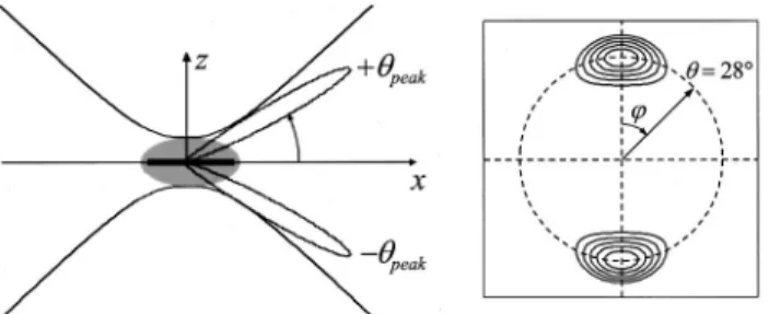
We now turn to the case of a collection of molecules driven by a field E and generalize the procedure described above to evaluate the resultant SHG radiation angular distribution and power. We restrict ourselves to the ge-ometry shown in Fig. 1, in which the dipoles are assumed to be uniformly distributed in a two-dimensional x – y plane (membrane plane) and illuminated by a highly fo-cused excitation beam propagating side-on in the xˆ direc-tion and polarized in the y – z plane (the fact that we use a side-on geometry rather than a head-on geometry will be-come evident). Our basic strategy consists in coarse-grain averaging the molecular dipole moments over mem-brane surface areas whose dimensions are small compared with the radiation wavelength but large enough to encompass large numbers of molecules. In this way we may define a local induced macroscopic dipole moment per unit molecular surface density:
2,i共x, y兲 ⫽1/2E2共x, y兲
兺
j,k 具
ijk典ˆjˆk, (7)
where E(x, y) is the complex amplitude of the driving
field at the position (x, y) on the membrane,⑀ˆ is its polar-ization direction,具典 symbolizes a local ensemble average of the molecular hyperpolarizabilities (we shall describe
this average in more detail below), and we have neglected local field effects. We emphasize that our term ‘‘macro-scopic’’ here is still microscopic relative to wavelength scales. Thus all the molecules taken in the coarse-grain average at a given position (x, y) are driven in phase with one another, and the net local dipole moment per unit area generated at this position is simply Ns2(x, y),
where Nsis the molecular surface density. The phase of
2(x, y) at different positions is determined by the phase
of the driving field E(x, y). To calculate the radiation generated by a global membrane surface, we then treat the local dipole moments at each position on the mem-brane plane as elemental radiators and coherently sum their radiated electric fields while taking their relative phases and amplitudes into account.
As we emphasized in Section 1, the excitation field can-not be regarded as a simple collimated beam here, and in-deed a full calculation that takes diffraction and polariza-tion into account shows that the field’s amplitude and phase cannot even be expressed analytically in the case of tight focusing.22 It has been shown, however, that as far
as nonlinear interactions are concerned one may closely approximate a tightly focused field by assuming that its amplitude is Gaussian in both the axial and the lateral di-rections about the focal center and that its phase near the focal center progresses linearly. That is, we can write
E共x, y兲 ⫽ ⫺iEexp
冉
⫺x2
wx2⫺ y2
wy2 ⫹ ikx
冊
, (8)where wx and wy are the axial and the lateral field
waists, respectively (explicit expressions for these may be found in App. B of Ref. 23), k⫽ n/c is the local wave vector, and is a parameter that characterizes the phase shift experienced by a Gaussian beam in the vicinity of a focal center. This phase shift is commonly referred to as a Gouy shift or a phase anomaly.22 In the case of weak focusing, may be approximated by (1 ⫺ 2/k2wy2),
whereas for tight focusing this expression tends to be a slight overestimate (see Appendix A). We emphasize
again that the field in Eq. (8) differs from a collimated beam in two respects: It experiences a local axial ampli-tude variation about the focal center as well as a phase shift. Both of these effects play a considerable role in the structure of the resultant SHG.
By adopting the coordinate system illustrated in Fig. 1, we proceed to calculate the second-harmonic far field ra-diated in the direction (, ). We begin by writing the contribution to the radiated electric field from the local in-duced polarization per unit molecular surface density and at the focal center only [indicated by the superscript (0);
2(0)⫽2(0, 0)]. This is given by E2共0兲共, 兲 ⫽
冉
E2 共0兲p共, 兲 E2共0兲s共, 兲冊
⫽ rM • 2 共0兲, (9) where ⫽2/0c2 and M is the projection matrix,
de-fined by M
冋
ˆˆ
册
⫽冋
⫺sin cos sin cos cos
0 cos ⫺sin
册
. (10) That is, E2p is the amplitude of E2in theˆ direction andE2s is the amplitude of E2in theˆ direction. The total
radiated field in the propagation direction (, ) is then given by the coherent summation of the contributions from the local induced polarization at all points x and y, with their associated spatially dependent phase shifts taken into account. We find then that
E2共, 兲 ⫽ Ns
r
冕 冕
M • 2共x, y兲⫻ exp关⫺ik2共x cos ⫹ y sin sin 兲兴dx dy, (11)
where k2⫽ 2n2/c. On integration, Eq. (11) yields E2共, 兲 ⫽ NA共, 兲E2共0兲共, 兲, (12)
where we have introduced the parameters
N⫽ 2wxwyNs, (13) A共, 兲 ⫽ exp
再
⫺k2 2 8 关wx 2共cos ⫺ ⬘兲2⫹ w y 2共sin sin 兲2兴冎
(14) and ⬘⫽ n/n2. The physical meanings of N andA(, ) are as follows: N defines the effective total
num-ber of molecules that contribute to the generation of second-harmonic light. This definition is identical to that detailed in Ref. 23 for two-photon excitation, though here it applies to a two-dimensional geometry. Accord-ingly, the effective total surface area that produces second-harmonic light is simply N/Ns. Because the
mol-ecules involved in SHG are spatially distributed on this surface area, the resultant angular profile of the SHG ra-diation is much more complicated in structure than that of a simple elemental radiator. In particular, we observe from Eq. (12) that the emission pattern of the SHG is the product of two terms: The first is the pattern that arises from an elemental dipole radiator E2(0)(, ) at the focal
Fig. 1. Coordinate system defining the SHG emission direction. The membrane surface (shaded; z⫽ 0) is approximated to be planar at the length scales considered. The focused excitation beam propagates in the ⫹x direction. The resultant SHG is mostly confined to an interaction area schematically depicted as a dotted ellipsoid and is radiated in the directions defined by and (thick arrow), with polarization components parallel to (E2p ) and perpendicular to (E
2
s ) the emission plane (shown
center, and the second is an angular modulation term de-fined by the scalar function A(, ). As we shall see be-low, the effect of the latter modulation term on the radiation structure is quite dramatic.
Finally, the radiated second-harmonic powers in the p and s polarization and in the solid angle defined by (, ) are given by
P2p,s共, 兲 ⫽ 1/2n
20cr2兩E2p,s共, 兲兩2, (15)
and the total radiated power obtained by integration over all angles becomes
PSHG⫽ PSHG p ⫹ P SHG s ⫽43n20c2N2 ⫻ 关⌰x2,x共0兲2 ⫹ ⌰y2,y共0兲2 ⫹ ⌰z2,z共0兲2兴, (16)
where we have introduced the angular structure param-eters ⌰x⫽ 3 8
冕
A 2共, 兲sin3dd, ⌰y⫽ 3 8冕
A2共, 兲关1 ⫺ sin2 sin2兴sindd,
(17) ⌰z⫽
3 8
冕
A2共, 兲关1 ⫺ sin2 cos2兴sindd.
The contributions to the total power from the various directional components of the induced second-harmonic dipoles are therefore readily identified. We note that if
A(, ) ⫽ 1, as is the case for a single elemental dipole
radiator, then⌰x⫽ ⌰y⫽ ⌰z⫽ 1.
C. Membrane Hyperpolarizability
In the derivation of Eqs. (15) and (16), no assumptions have been made about the dipole vector2(0), which may be taken as arbitrary. For our considerations, however, we shall assume that2(0)is generated by molecules that are quasi-uniaxial. That is, if we define a coordinate sys-tem (X, Y, Z) that is proper to a molecule, then the mo-lecular first hyperpolarizability is dominated largely by the single component zzz. Moreover, we assume that
the molecules are preferentially aligned in the lipid mem-brane such that, on average, the molecular Z axis is in the same direction as the z axis defined by the membrane, though we do not otherwise specify the distribution that governs tilt angles␣.
The molecular X and Y axes, in turn, are assumed to be uniformly randomly oriented. In particular, we discount any possible correlation between the X and Y orientations and tilt angle ␣. With the above assumptions in mind, we may derive a coarse-grained local ensemble average for the hyperpolarizability that is valid over regions whose dimensions are small compared with the optical wavelength but large enough to encompass a large num-ber of molecules. Expressed in the membrane coordinate system (x, y, z), the nonzero components of this first hy-perpolarizability are given by
xxz⫽xzx⫽yyz⫽ yzy⬅⫹,
xyz⫽xzy⫽ ⫺yxz⫽ ⫺yzx⬅ ⫺,
zxx⫽zyy⬅t,
zzz⬅z, (18)
where we have used the definitions
⫹⫽具cos3␣典B⫹⫹ 1/2具sin2␣ cos ␣典共BZ⫺ BT兲,
⫺⫽1/2具3 cos2␣ ⫺ 1典B⫺,
t⫽具cos3␣典BT⫹ 1/2具sin2␣ cos ␣典共BZ⫹ BT ⫺ 2B⫹兲,
z⫽具cos3␣典BZ⫹ 具sin2␣ cos ␣典共BT ⫹ 2B⫹兲, (19)
where具 典 signifies an ensemble average and
B⫹⫽1/2共 XXZ⫹ YYZ兲, B⫺⫽1/2共 XYZ⫺YXZ兲, BT⫽1/2共ZXX⫹ ZYY兲, BZ⫽ZZZ. (20)
Having derived the effective molecular hyperpolariz-ability in the membrane frame, we may now derive the induced second-harmonic dipole at the focal center 2(0) from Eq. (7). We consider the case when the driving field is polarized in the y – z plane and write ˆ ⫽ (0, sin, cos ), where represents the inclination of the polarization direction from the z axis. A straightfor-ward application of Eqs. (7) and (18) then yields
2共0兲⫽1/2E2共⫺sin 2, ⫹sin 2, zcos2 ⫹ tsin2兲.
(21) Finally, by inserting Eq. (21) into Eqs. (9), (12), and (15), we obtain the p and s polarization components of the radiated second-harmonic power.
D. Uniaxial Hyperpolarizability
To distill the basic features of our results, we restrict our-selves here to the simplifying case in which the molecules in the membrane are perfectly oriented in the zˆ direction (i.e.,␣ ⫽ 0) and strictly uniaxial, such that the only non-zero component to the molecular first hyperpolarizability is ZZZ (i.e., ⫹⫽⫺⫽ t⫽ 0; z⫽ZZZ). We also
begin by considering the case in which the driving field is polarized in the zˆ direction (i.e., ⫽ 0). This is the same case as examined in subsection 2.A for a single mol-ecule, with the only difference being that here we consider the effects of a planar distribution of molecules. As be-fore, we find at the focal center
2共0兲⫽ 1/2zE2zˆ, (22)
which again is the induced dipole moment per unit mo-lecular surface density. The radiated power from the dis-tribution of induced dipole moments about the focal cen-ter, expressed in photons/second, is then given by
P2p 共, 兲 ⫽ 163 SHGN2A2共, 兲cos2 cos2I2, (23) P2s 共, 兲 ⫽ 3 16 SHGN 2A2共, 兲sin2I 2, (24)
and the integrated total power is
PSHG⫽1/2⌰zN2SHGI2. (25)
For a single radiating dipole, ⌰z⫽ 1; however, for a
distribution of many dipoles,⌰z⬍ 1 in general. The
an-gular pattern of the radiated SHG light is governed mainly by the function A(, ). The structure of A(, ) critically depends on the interaction area and on⬘ and exhibits two symmetric peaks, atpeak⫽ ⫾cos⫺1(⬘) (Fig.
2). This bidirectional nature of the SHG stems from the fact that the excitation light is subject to an effective in-crease in wavelength owing to the phase anomaly near the focal center. As a result, the SHG radiation must be emitted at an angle ⫾peak relative to the excitation
propagation direction to be properly phase matched. We assume throughout this paper that is roughly constant within the SHG excitation area. This approximation is justified in Appendix A. We emphasize here that is in-timately linked to the interaction area and may not be re-garded as an independent parameter. When the interac-tion area is reduced, then so too is , which leads to a widening of the angular separation between the two lobes as well as a broadening of the lobes themselves. In par-ticular, a reduction in the axial and lateral waists of the excitation beam leads to a broadening of the lobe profiles along the and directions, roughly respectively.
A direct comparison can be made between the total powers emitted in the cases of SHG and TPEF. Noting that the total TPEF power scales with N, we find that
PSHG PTPEF ⫽ 2
冑
2⌰zN SHG TPEF , (26)where the factor 2
冑
2 stems from the volume contrast of a three-dimensionally Gaussian fluorescence excitation volume.23Because the SHG radiation is emitted into two well-defined lobes, small-angle approximations about ⬇ ⫾peakand ⬇ 0 may be used to provide an estimate
of the structure parameter⌰z. A straightforward
evalu-ation of Eqs. (17) with these approximevalu-ations yields
⌰z⬇
3⬘2
k22 wxwy
冑
1⫺⬘2. (27)
Bearing in mind the approximate dependence of the focal area on the numerical aperture (NA) of the excitation beam (wx⬃ NA⫺2; wy⬃ NA⫺1), we can infer the
follow-ing relations: N⬃ NA⫺3, I⬃ NA2, and for low NA we
can approximate ⌰z⬃ NA2 (see Appendix A). We find
then that the total emitted SHG power is roughly inde-pendent of NA for NA⬍ 0.8. For higher NA’s, the SHG power diminishes. In comparison, the total emitted TPEF power scales as NA in a two-dimensional geometry.
E. Polarization Anisotropy
In our discussions so far we have assumed that the mem-brane geometry was planar. In our experiments, how-ever, the membranes are in fact spherical, with diameters typically in the 20–50-m range. The excitation beam waist at the focal center is typically of submicrometer size; hence the assumption that the membrane is planar over this dimension is entirely valid. We note, however, that the membrane coordinate frame as defined above is not the same as the laboratory coordinate frame. In par-ticular, if the excitation beam polarization is linear and fixed in the laboratory frame, it will appear to tilt in the membrane frame, depending on which portion of the membrane surface is illuminated. If we scan only along an equatorial cross section of the membrane, the polariza-tion direcpolariza-tion will rotate relative to the membrane’s z axis with an angle, which spans 0 to 2. In the case of per-fectly aligned uniaxial molecules (⫹⫽ ⫺⫽t⫽ 0),
the induced local dipole moment for an angle as ob-tained from Eq. (21) is simply
2共0兲⫽ 1/2E2共0, 0,zcos2兲. (28)
The resultant p and s polarizations of the radiated field in the local membrane coordinate frame are then obtained from Eq. (9), and the total radiation power generated lo-cally along the membrane equator is found to vary as cos4.
Experimentally it is difficult to isolate the p and s com-ponents of the radiated field because these are not fixed in the laboratory frame. We can transform them, however, into orthogonal polarization components, which are fixed in the laboratory frame through the relation
冉
E2储 E⬜2冊
⫽冋
cos共 ⫺兲 ⫺sin共 ⫺ 兲 sin共 ⫺兲 cos共 ⫺ 兲册
冉
E2p E2s冊
. (29)Here E2储 and E⬜2 represent the radiated electric field components parallel and perpendicular, respectively, to the excitation beam’s polarization direction. These latter polarization components can be isolated quite simply, as is shown below.
Following steps similar to those used in deriving Eq. (16), we can derive the total radiated SHG powers along the储and⬜ polarizations. These are given by
Fig. 2. Left, an excitation beam propagating in the x direction and polarized along the z axis is focused (side-on) onto the mem-brane of a labeled lipid vesicle. Only a small surface area (thick segment; side view) of this much larger vesicle contributes to SHG. Phase matching between the SHG and excitation fields causes the SHG radiation to be double peaked in the forward di-rection. Right, far-field power distribution of the SHG radia-tion.
PSHG储 ⫽ 4 3 n20c 2N2 2,z 共0兲2关共⌰ z ⫺ 2⌰z⬘兲cos2 ⫹ ⌰z⬘兴, (30) P⬜SHG⫽ 4 3 n20c 2N2 2,z 共0兲2关共⌰ z⫺ 2⌰z⬘兲sin2 ⫹ ⌰z⬘兴, (31) where we have introduced the auxiliary angular structure parameter
⌰z⬘⫽
3 8
冕
A2共, 兲
⫻ 关共1 ⫺ cos兲2sin2 cos2兴sindd. (32)
Although the above relations are exact, in most cases of interest⌰z⬘is considerably smaller than⌰zand can safely
be neglected. We then find that the powers emitted into the orthogonal polarization components PSHG储 and P⬜SHG
vary, respectively, as cos6 and cos4 sin2 along the
membrane equator. We emphasize that the above re-sults apply to rigorously uniaxial and well-oriented mol-ecules only. In practice, not all molmol-ecules have these at-tributes, as will be seen below.
3. SHG CROSS SECTION
The molecule used in our experimental investigation is the lipophilic styryl dye N-(4-sulfobutyl)-4-(4-(dihexyl-amino)styryl)pyridinium (Di-6-ASPBS). The donor–( -bridge)–acceptor structure of this molecule permits sig-nificant charge transfer along its major Z axis, resulting in a large first hyperpolarizability component ZZZ.24–26
Donor–(-bridge)–acceptor molecules have been found to be well described by a two-state model.15,27 When driven
near resonance,ZZZ may be approximated by
ZZZ共⫺2, , 兲 ⫽ 2 ប2eg2 ⌬
冋
1 共eg⫺ 2 ⫹ i⌫兲共eg⫺ ⫹ i⌫兲 ⫹ 1 共eg⫺ ⫹ i⌫兲共eg⫹ ⫺ i⌫兲 ⫹ 1 共eg⫹ 2 ⫺ i⌫兲共eg⫹ ⫺ i⌫兲册
, (33) where eg and eg are, respectively, the transitionfre-quency and the dipole transition moment, ⌬ is the dif-ference between excited-state and ground-state dipole moments and⌫ is a phenomenological damping constant. Although no direct experimental measurements of ZZZ
in membrane are available, the absorption spectrum of Di-6-ASPBS in membrane allows us to infer a charge transfer energy បeg⫽ 2.56 eV, a transition moment
eg⬇ 10 D, and a damping factor ⌫ ⬇ 0.19 eV, all
spe-cific to a membrane environment. In addition, previous electrochromism measurements of similar dyes in membrane28 allow us to estimate that ⌬ ⬇ 16 D for Di-6-ASPBS. We may therefore predict a large static first hyperpolarizability of roughly (0) ⬇ 2 ⫻ 10⫺48C m3V⫺2. This value is enhanced when the
molecule is excited near resonance. In particular, for an
excitation wavelength of 880 nm, we find that  ⬇ 1 ⫻ 10⫺47C m3V⫺2, or, equivalently,
SHG⬇ 1
⫻ 10⫺3GM (1 GM ⫽ 10⫺50cm4/photon s⫺1). For
com-parison, the TPEF cross section of Di-6-ASPBS in mem-brane at the same excitation wavelength has been esti-mated to be TPEF⬇ 30 GM, based on TPEF
measurements in ethanol. We note that, despite the fact that SHGis⬃4 orders of magnitude smaller thanTPEF
for a single molecule, we may benefit from the fact that SHG field amplitudes add coherently in the case of a large number of molecules, as shown in Eq. (26). In practice and for standard dye labeling densities, we can easily ob-tain SHG and TPEF powers that are comparable, as we show below.
4. EXPERIMENTAL ANALYSIS
A. SHG and TPEF Imaging of Membranes
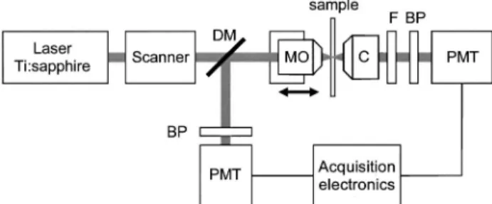
Our experimental apparatus is a home-built scanning SHG TPEF microscope, the basics of which are shown in Fig. 3. The excitation source is a mode-locked Ti:sap-phire laser (Spectra-Physics), which delivers ⬃80-fs pulses at an 81-MHz repetition rate. The laser light is focused into the sample with a water-immersion micro-scope objective (Olympus, LUMPlanFL60⫻W/IR) and the resultant SHG is collected in the forward direction, while the TPEF is collected in the backward direction. Our sample consists of giant unilamellar vesicles (GUV’s) made from a pure lipid in water. These serve as model systems for the study of SHG radiation from membrane surfaces. The lipid type is 1,2-dioleoyl-sn-glycero-3-phosphocholine (Avanti, DOPC), which is in the fluid phase L␣at room temperature. The vesicles are labeled at 1 mol. % with Di-6-ASPBS; preparation and labeling are described elsewhere.29 Calcium ions are added to promote adhesion between adjacent vesicles, and the glass slide is coated with poly-L-lysine (Sigma P8920) to prevent sticking and bursting.
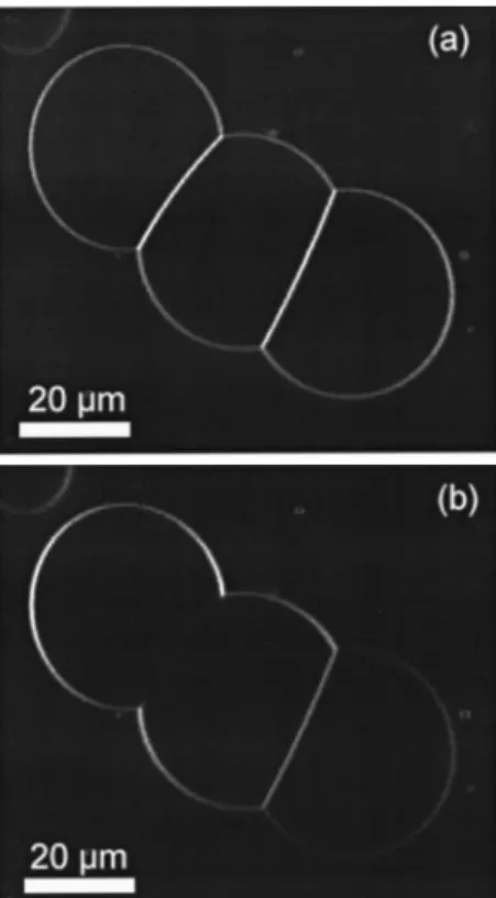
Figure 4 shows SHG and TPEF images of three GUV’s of nearly equal radii that have adhered to form a foam. The GUV’s are labeled with Di-6-ASPBS and acquired un-der the conditions described above. SHG scales with the
Fig. 3. Experimental layout: a Ti:sapphire laser beam is fo-cused into a sample with a microscope objective (MO). The transmitted SHG is collected with a condenser (C), bandpass (BP) filtered, and detected with a photomultiplier tube (PMT). The transmitted laser light is blocked with a colored glass filter (F). The TPEF from the sample is epicollected, discriminated with a dichroic mirror (DM), bandpass (BP) filtered, and detected with a PMT. Three-dimensional images are formed by scanning the laser focal spot in the lateral directions with galvanometer-mounted mirrors, and in the axial direction by translating the MO.
square of the excitation intensity and hence leads to the same intrinsic three-dimensional resolution as TPEF, here 510 nm lateral and 1.9 m axial. An excitation power of less than 1 mW at the sample provides approxi-mately equal measured powers for both SHG and TPEF, allowing the images to be acquired simultaneously with integration times of ⬃10 s/pixel. The measured radi-ated powers are in good agreement with those predicted by the model developed in Section 3. In particular, if we estimate our dye surface density to be Ns⫽ 1.5
⫻ 1016m⫺2, and take into account the fact that
essen-tially all the SHG light is collected because it is highly di-rectional whereas only⬃20% of the radiated fluorescence is epicollected, we find that PSHG/PTPEF⬇ 0.5. To
con-firm that the light collected in the forward direction is in-deed SHG in origin, we routed both the forward and the backward signals into a spectrograph. The SHG spec-trum revealed a sharp peak at 440 nm, whereas the TPEF spectrum was broadly distributed about 580 nm.18 The leftmost two vesicles in Fig. 4(a) have nearly equal TPEF brightness; the third vesicle is less bright, presumably owing to reduced labeling. Because SHG scales with the square of the label surface density, the contrast between the two bright vesicles and the third, dimmer, vesicle is enhanced in Fig. 4(b). We also clearly illustrate here the coherent nature of SHG radiation, as opposed to the inco-herent nature of TPEF. In regions where the dipole dis-tributions are symmetric, such as in the adhesion zones
between the adjacent vesicles, the SHG vanishes, whereas the TPEF does not. We note that the cancella-tion of SHG is almost perfect in the left zone. It is less perfect in the right zone owing to the disparity in the sur-face labeling density.
B. SHG Radiation Pattern
To characterize the angular pattern of the SHG radiation we removed the condenser from our collection optics and replaced it with an oil-immersion microscope objective (Olympus, UPlanFL60⫻1.25 Oil Iris). We then imaged the back aperture of this objective onto a CCD camera (Cohu 4912/Scion Corporation LG-3 frame grabber). This allowed us to visualize directly the emission angle. Figure 5 illustrates the SHG radiation pattern obtained when the laser scanning was restricted to a small patch of membrane on the equatorial slice of a vesicle. The aver-age power at the focus was maintained below 5 mW, per-mitting a CCD integration time of⬃5 ms/pixel. The two lobes that occur at ⫾peakare manifest. These are the
emission directions that correspond to phase matching of the SHG and excitation fields, as predicted by theory. As shown, however, the two lobes are not perfectly cylindri-cally symmetric about ⫽ 0. In particular, the left lobe curves outward rather than inward. This may be the re-sult of the local membrane curvature, which is not taken into account in our theory. In particular, when the mem-brane curvature was reversed, the lobe symmetry also be-came reversed. We also point out that there was a slight index-of-refraction mismatch between the insides and the outsides of our vesicles. As a result, the lobe that is di-rected toward the inside of a vesicle experiences a slight distortion owing to the lensing effect when it exits the vesicle, which may further contribute to the observed asymmetry in the lobes.
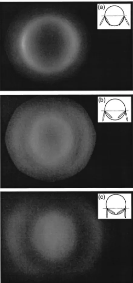
When the laser was allowed to scan over an entire vesicle cross section, the angular radiation pattern be-came annular, as shown in Fig. 6. The radiation pattern was observed to be highly sensitive to the inclination of the local membrane plane relative to the propagation axis. For example, in images generated from cross
sec-Fig. 4. Simultaneous (a) TPEF and (b) SHG images of three vesicles labeled with Di-6-ASPBS that have adhered to form a foam. The radiating Di-6-ASPBS molecules are more-or-less symmetrically distributed in the adherence regions between the vesicles. In the left region, a symmetric distribution results in a nearly perfect cancellation of SHG. In the right region, the can-cellation is imperfect because of a disparity in labeling density. As opposed to SHG radiation, TPEF is independent of molecular distribution because it is incoherent.
Fig. 5. CCD image of the back aperture of the SHG collection objective. The excitation beam is scanned only over a small por-tion of an equatorial slice of a GUV membrane. The double-peaked angular distribution of the SHG radiation is apparent.
tions below the equatorial plane, two annular rings be-came apparent. The origin of these rings is made clear in Fig. 6. We note that the radius of the annular ring ob-tained from the equatorial plane provides a precise deter-mination ofpeak. In our case, from Fig. 6(a) and
correct-ing for the index mismatch that is caused by the condenser glass, we find experimentallypeak⬇ 24°,
cor-responding to ⬘⬇ 0.91. This value of
⬘
is somewhat larger than that predicted from numerical calculations (see Appendix A). A possible reason for this discrepancy is that, as mentioned above, one lobe experiences a slight deviation on transit through the vesicle while the other does not. Furthermore, we assumed in our calculations that the back aperture of the excitation objective was completely and uniformly filled. Such was not the case in practice, meaning that our focal spot was probably somewhat larger than specified.C. SHG Polarization Analysis
To conclude our experimental analysis, we briefly exam-ine some polarization anisotropy properties of the SHG radiation obtained from vesicle membranes. In particu-lar, we consider the case in which the excitation light is linearly polarized and we can select the corresponding parallel and cross-polarized components of the detected
SHG radiation. We perform this selection simply by in-serting a linear polarizer between the condenser and the SHG detection photomultiplier tube in Fig. 2. Depend-ing on the orientation of this polarizer relative to the ex-citation polarization detection, we can effectively isolate the PSHG储 and P⬜SHGcomponents of the SHG radiation, as
described in Subsection 2.E. Our results, for example, for Di-6-ASPBS labeling of GUV’s are presented in Fig. 7. We note that we do not fully recover the respective cos6
and cos4 sin2 angular dependencies for PSHG储 and
P⬜SHG, as predicted from our simplified model. Though
there may be several explanations for this, the most prob-able is that the assumptions that Di-6-ASPBS is strictly uniaxial and that it is perfectly aligned in the zˆ direction when it is inserted into a membrane are overly simplistic. For example, it has been suggested30 that a molecule closely related to Di-6-ASPBS may possess a significant transverse polarizability component BT in the molecule
frame [and hence t in the membrane frame; see Eqs.
(18)–(20)]. Such a transverse component would add a sin2 component to
2,z
(0) and hence would significantly
modify the expected angular dependencies of PSHG储 and
P⬜SHG, yielding a closer fit to experiment. Moreover, even in the case of a rigorously uniaxial polarizability, any de-viations from perfect alignment would further complicate matters by introducing a nonzero 2,y(0) component. Fi-nally, we assumed in Subsection 2.E that the active SHG surface area remained constant everywhere along the membrane equator; that is, we assumed that wz⫽ wyin
the focal plane and that the two waist dimensions could be freely interchanged. This is not strictly true in the case of a linearly polarized excitation beam.
Suffice it to say that a full polarization analysis of the SHG radiation from membranes remains rather complex owing to the many possible hyperpolarizability compo-nents that may be involved, as evidenced by Eqs. (18)– (20). Such a comprehensive analysis is beyond the scope of this paper.
Fig. 6. Stack of CCD images of the back aperture of the SHG collection objective. The excitation beam, incident from above in the insets, is scanned through full cross sections of a GUV at various latitudes. The equatorial cross section is scanned for image (a), leading to a single annular ring atpeak, whereas lati-tudes below the equator are scanned for images (b) and (c). The CCD images were integrated over times long enough to permit multiple scans. From image (a) we deduce thatpeak ⬇ 24°.
Fig. 7. Variation of SHG power along the equator of a GUV la-beled with Di-6-ASPBS. Excitation is linearly polarized. A po-larizer is inserted in the detection path and is oriented parallel (PSHG储 ) or perpendicular (P⬜SHG) to the excitation polarization. Plots are shown as a function of anglebetween the normal to the membrane plane (z axis) and the excitation polarization di-rection. The dashed trace corresponds to the cos6dependence
5. CONCLUSION
Our purpose in this paper was to lay some theoretical foundations for high-resolution SHG imaging of mem-branes. Inasmuch as SHG imaging may be performed si-multaneously with TPEF imaging, we have taken par-ticular care to establish a formalism that permits direct comparison between the two modalities. Similarities be-tween SHG and TPEF emission powers are that both scale with the square of the excitation intensity, that they may both be defined in terms of commensurate molecular cross sections, and that their active focal areas (or vol-umes) are independent of the sample size and depend only on the focus tightness. Differences lie in the fact that SHG power scales with the square of the number of molecules, whereas TPEF power scales only linearly with number. Moreover, a structure parameter is necessary for proper quantification of SHG power, which depends on the extent of the active focal area. We note finally that our formalism, which is essentially derived from regard-ing a distribution of hyperpolarizable molecules as a phased-array antenna, is readily extendible to the gen-eration of harmonics of higher order. In all these cases, effective molecular cross sections may be rigorously de-fined, and an active focal area (or volume, as in the case of third-harmonic generation in bulk) may be readily identi-fied.
APPENDIX A
A general theoretical framework for describing the elec-tromagnetic field near the focus of a tightly focused beam has been proposed by Richard and Wolf.31 This
frame-work, based on diffraction theory, may be applied to lin-ear or nonlinlin-ear optical microscopy. In the case of TPEF microscopy, the signals are incoherent, and only the local field intensity, or correspondingly the field amplitude, need be calculated about the focal center. In the case of SHG microscopy, however, the signals are coherent, and the situation becomes more complicated. Both the local field amplitude and phase must be calculated about the focal center.
It is well known that any focused beam incurs a net phase shift after it passes through its focus. This phe-nomenon, commonly referred to as a phase anomaly, has a profound influence on the spatial structure of SHG ra-diation from a membrane. On closer inspection the phase shift, which is /2 exactly at the focal center, is found to vary approximately linearly with distance along the propagation axis near the focal center. As such, a fo-cused beam behaves much as a plane wave near the focal center, though with an effective wave vector that has been modified relative to that of an unfocused beam. The effective wave vector of a focused beam near its focal cen-ter may be written ask, where kis the wave vector of
a corresponding unfocused beam and in general is less than 1. Because the phase of the induced second-harmonic polarizability is governed by the phase of the excitation field, and because appreciable SHG power is produced only in directions that permit proper phase matching between this induced polarizability and the re-sultant SHG field, we find that, because ⬍ 1, the
radi-ated SHG power in the forward ( ⫽ 0) direction is weak. The radiated SHG power along ⫽ ⫾peak, however, is
appreciable because the fields in these directions are in phase and add coherently. Bothpeakand the total
radi-ated SHG power depend critically on ; hence a detailed evaluation of this parameter is warranted.
We use the integral formulas derived in Ref. 22 to ex-amine how varies with the NA of the focusing objective of the excitation beam. To begin, we evaluate only at the focal center and consider the case n2⬇ n. We may define a focusing angleNA⫽ sin⫺1(NA/n) to
char-acterize the angular range of the excitation light. A com-parison of peak⫽ cos⫺1() and NA for several NA’s is
shown in Fig. 8. We observe that peak/NA is roughly
constant and less than 1, from which we obtain the gen-eral rule of thumb that a collection NA equal to the exci-tation NA is sufficient for essentially all the SHG light to be collected. In particular, for low NA’s we find that
Fig. 8. Variations of the ratio peak/NA [where NA ⫽ sin⫺1(NA/n)] and of the parameter (1⫺2)1/2/2as a
func-tion of the NA of a water-immersion microscope objective, assum-ing a uniformly backfilled aperture and linear polarization. The plots are obtained from full numerical evaluations valid for arbi-trary NA. For low NA,peak→NA/冑2.
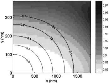
Fig. 9. Spatial profile of the phase-anomaly parameter (shades) and of the normalized intensity-squared distribution (contours) about the focal center (0, 0) of an 880-nm-wavelength laser beam focused by water-immersion objective with a NA of 0.9. The axial propagation direction is x; the lateral direction is y. Profiles were calculated assuming a uniformly backfilled ap-erture and linear polarization. is relatively constant within the major portion of the intensity-squared profile.
peak⫽NA/
冑
2. We also provide a plot of the parameter(1⫺ 2)1/2/2 as found in expression (27). This
param-eter is found to vary linearly with NA for low to modest NA’s.
Finally, throughout this paper we have assumed that is roughly constant over the entire membrane surface area that contributes to SHG radiation. To justify this assumption we illustrate the numerical evaluation of the (x, y) near the focal center and compare this with the corresponding intensity distribution of the excitation beam (Fig. 9) for our experimental case of interest (NA of 0.9). We observe that varies only slightly within the major portion of the intensity-squared distribution, and hence the approximation that is constant over the active surface area in which SHG is produced is quite reason-able. In our case, we find numerically that ⬇ 0.88.
ACKNOWLEDGMENTS
The authors gratefully acknowledge financial support by the Insitut Curie and by the Centre National de Recher-che Scientifique. We thank M. Blanchard-Desce for pro-viding the dye molecules and S. Charpak and C. Boccara for helpful assistance. L. Moreaux was supported by a
Bourse Docteur Inge´nieur.
J. Mertz’s e-mail address is [email protected].
REFERENCES
1. W. Denk, J. H. Strickler, and W. W. Webb, ‘‘Two-photon la-ser scanning fluorescence microscopy,’’ Science 248, 73–76 (1990).
2. J. R. Lakowicz and I. Gryczynski, ‘‘Multiphoton excitation of biochemical fluorophores,’’ in Topics in Fluorescence Spectroscopy, J. R. Lakowicz, ed. (Plenum, New York, 1997), Vol. 5, p. 87.
3. C. Xu and W. W. Webb, ‘‘Multiphoton excitation of molecu-lar fluorophores and nonlinear laser microscopy,’’ in Topics in Fluorescence Spectroscopy, J. R. Lakowicz, ed. (Plenum, New York, 1997), Vol. 5, p. 471.
4. S. Maiti, J. B. Shear, R. M. Williams, W. R. Zipfel, and W. W. Webb, ‘‘Measuring serotonin distribution in live cells with three-photon excitation,’’ Science 24, 530–532 (1997). 5. C. Xu, W. Zipfel, J. B. Shear, R. M. Williams, and W. W. Webb, ‘‘Multiphoton fluorescence excitation: new spectral windows for biological nonlinear microscopy,’’ Proc. Natl. Acad. Sci. USA 93, 10,763–10,768 (1996).
6. J. I. Dadap, J. Shan, A. S. Weling, J. A. Misewich, A. Na-hata, and T. F. Heinz, ‘‘Measurement of the vector charac-ter of electric fields by optical second-harmonic generation,’’ Opt. Lett. 24, 1059–1061 (1999).
7. R. Gauderon, P. B. Lukins, and C. J. R. Sheppard, ‘‘Three-dimensional second-harmonic generation imaging with femtosecond laser pulses,’’ Opt. Lett. 23, 1209–1211 (1998). 8. Y. Guo, P. P. Ho, H. Savage, D. Harris, P. Sacks, S. Schantz, F. Liu, N. Zhadin, and R. R. Alfano, ‘‘Second-harmonic tomography of tissues,’’ Opt. Lett. 22, 1323–1325 (1997).
9. G. Peleg, A. Lewis, M. Linial, and L. M. Loew, ‘‘Non-linear optical measurement of membrane potential around single molecules at selected cellular sites,’’ Proc. Natl. Acad. Sci. USA 96, 6700–6704 (1999).
10. P. J. Campagnola, M. Wei, A. Lewis, and L. M. Loew,
‘‘High-resolution nonlinear optical imaging of live cells by second harmonic generation,’’ Biophys. J. 77, 3341–3349 (1999).
11. D. Yelin and Y. Silberberg, ‘‘Laser scanning third-harmonic-generation microscopy in biology,’’ Opt. Express
5, 169–175 (1999).
12. M. Muller, J. Squier, K. R. Wilson, and G. J. Brakenhoff, ‘‘3D-microscopy of transparent objects using third-harmonic generation,’’ J. Microsc. 191, 266–269 (1998). 13. T. F. Heinz, H. W. K. Tom, and Y. R. Shen, ‘‘Determination
of molecular orientation of monolayer adsorbates by optical second-harmonic generation,’’ Phys. Rev. A 28, 1883–1885 (1983).
14. N. Bloembergen, ‘‘Second harmonic reflected light,’’ Opt. Acta 13, 311–322 (1966).
15. Y. R. Shen, The Principles of Nonlinear Optics (Wiley, New York, 1984).
16. R. Boyd, Nonlinear Optics (Academic, London, 1992). 17. A. Lewis, A. Khatchatouriants, M. Treinin, Z. Chen, G.
Pe-leg, N. Friedman, O. Bouetvich, Z. Rothman, L. Loew, and M. Sheres, ‘‘Second-harmonic generation of biological inter-faces: probing the membrane protein bacteriorhodopsin and imaging membrane potential around GFP molecules at specific sites in neuronal cells of C. elegans,’’ Chem. Phys.
245, 133–144 (1999).
18. L. Moreaux, O. Sandre, M. Blanchard-Desce, and J. Mertz, ‘‘Membrane imaging by simultaneous second-harmonic gen-eration and two photon microscopy,’’ Opt. Lett. 25, 320–322 (2000).
19. A. Willets, J. E. Rice, D. Burland, and D. P. Shelton, ‘‘Prob-lems in the comparison of theoretical and experimental hy-perpolarizabilities,’’ J. Chem. Phys. 97, 7590–7599 (1992). 20. C. Xu and W. W. Webb, ‘‘Measurement of two-photon
exci-tation cross section of molecular fluorophores with data from 690 nm to 1050 nm,’’ J. Opt. Soc. Am. B 13, 481–491 (1996).
21. N. Bloembergen, Nonlinear Optics, 4th ed. (World Scien-tific, Singapore, 1965).
22. M. Born and E. Wolf, Principles of Optics, 6th ed. (Perga-mon, Oxford, 1993).
23. J. Mertz, ‘‘Molecular photodynamics involved in multi-photon excitation fluorescence microscopy,’’ Eur. Phys. J. D
3, 53–66 (1998).
24. S. R. Marder, D. N. Beratan, and L.-T. Cheng, ‘‘Approaches for optimizing the first hyperpolarizability of conjugated or-ganic molecules,’’ Science 252, 103–106 (1991).
25. T. Kogej, D. Beljonne, F. Meyers, J. W. Perry, S. R. Marder, and J. L. Bre´das, ‘‘Mechanisms for enhancement of two-photon absorption in donor–acceptor conjugated chro-mophores,’’ Chem. Phys. Lett. 298, 1–6 (1998).
26. D. S. Chemla and J. Zyss, Nonlinear Optical Properties of Organic Molecules and Crystals (Academic, New York, 1984).
27. J. L. Oudar, ‘‘Optical nonlinearities of conjugated mol-ecules. Stilbene derivatives and highly polar aromatic compounds,’’ J. Chem. Phys. 67, 446–457 (1977).
28. L. M. Loew and L. L. Simpson, ‘‘Charge shift probes of membrane potential. A probable electrochromic mecha-nism for ASP probes on a hemispherical lipid bilayer,’’ Bio-phys. J. 34, 353–365 (1981).
29. O. Sandre, L. Moreaux, and F. Brochard, ‘‘Dynamics of transient pores in stretched vesicles,’’ Proc. Natl. Acad. Sci. USA 96, 10,588–10,596 (1999).
30. C. W. Dirk, R. J. Twieg, and G. Wagnie´re, ‘‘The contribution of electrons to second harmonic generation in organic molecules,’’ J. Am. Chem. Soc. 108, 5387–5395 (1986). 31. B. Richards and E. Wolf, ‘‘Electromagnetic diffraction in
op-tical systems. II. Structure of the image field in aplanetic system,’’ Proc. R. Soc. London, Ser. A 253, 358–379 (1959).