HAL Id: hal-01096296
https://hal.archives-ouvertes.fr/hal-01096296
Submitted on 27 Dec 2014
HAL is a multi-disciplinary open access
archive for the deposit and dissemination of
sci-entific research documents, whether they are
pub-lished or not. The documents may come from
teaching and research institutions in France or
abroad, or from public or private research centers.
L’archive ouverte pluridisciplinaire HAL, est
destinée au dépôt et à la diffusion de documents
scientifiques de niveau recherche, publiés ou non,
émanant des établissements d’enseignement et de
recherche français ou étrangers, des laboratoires
publics ou privés.
Impact of the LMDZ atmospheric grid configuration on
the climate and sensitivity of the IPSL-CM5A coupled
model
Frédéric Hourdin, Marie-Alice Foujols, Francis Codron, Virginie Guemas,
Jean-Louis Dufresne, Sandrine Bony, Sébastien Denvil, Lionel Guez, François
Lott, Josefine Ghattas, et al.
To cite this version:
Frédéric Hourdin, Marie-Alice Foujols, Francis Codron, Virginie Guemas, Jean-Louis Dufresne, et al..
Impact of the LMDZ atmospheric grid configuration on the climate and sensitivity of the IPSL-CM5A
coupled model. Climate Dynamics, Springer Verlag, 2013, 40 (9-10), pp.2167-2192.
�10.1007/s00382-012-1411-3�. �hal-01096296�
(will be inserted by the editor)
Impact of the LMDZ atmospheric grid configuration
on the climate and sensitivity of the IPSL-CM5A
coupled model
Fr´ed´eric Hourdin · Marie-Alice Foujols · Francis Codron · Virginie Guemas · Jean-Louis Dufresne · Sandrine Bony · S´ebastien Denvil · Lionel Guez · Franccois Lott · Josefine Ghattas · Pascale
Braconnot · Olivier Marti · Yann Meurdesoif · Laurent Bopp
Received: date / Accepted: 26/05/2012
Abstract The IPSL-CM5A climate model was used to perform a large number
1
of control, historical and climate change simulations in the frame of CMIP5. The
2
refined horizontal and vertical grid of the atmospheric component, LMDZ,
con-3
stitutes a major difference compared to the previous IPSL-CM4 version used for
4
CMIP3. From imposed-SST (Sea Surface Temperature) and coupled numerical
ex-5
periments, we systematically analyze the impact of the horizontal and vertical grid
6
resolution on the simulated climate. The refinement of the horizontal grid results
7
in a systematic reduction of major biases in the mean tropospheric structures and
8
SST. The mid-latitude jets, located too close to the equator with the coarsest grids,
9
move poleward. This robust feature is accompanied by a drying at mid-latitudes
10
and a reduction of cold biases in mid-latitudes relative to the equator. The model
11
was also extended to the stratosphere by increasing the number of layers on the
ver-12
tical from 19 to 39 (15 in the stratosphere) and adding relevant parameterizations.
13
The 39-layer version captures the dominant modes of the stratospheric variability
14
and exhibits stratospheric sudden warmings. Changing either the vertical or
hor-15
izontal resolution modifies the global energy balance in imposed-SST simulations
16
by typically several W/m2which translates in the coupled atmosphere-ocean
sim-17
ulations into a different global-mean SST. The sensitivity is of about 1.2 K per
18
1 W/m2 when varying the horizontal grid. A re-tuning of model parameters was
19
F. Author
Laboratoire de M´et´eorologie Dynamique, IPSL UPMC, Tr 45-55, 3e et, B99
Jussieu, 75005 Paris
E-mail: hourdin@lmd.jussieu.fr
F. Codron, V. Guemas, J.-L. Dufresne, S. Bony, L. Guez, F. Lott LMD
M.-A. Foujols, S. Denvil, J. Gatthas IPSL
P. Braconnot, O. Marti, Y. Meudesoif, L. Bopp LSCE
thus required to restore this energy balance in the imposed-SST simulations and
20
reduce the biases in the simulated mean surface temperature and, to some extent,
21
latitudinal SST variations in the coupled experiments for the modern climate. The
22
tuning hardly compensates, however, for robust biases of the coupled model.
De-23
spite the wide range of grid configurations explored and their significant impact
24
on the present-day climate, the climate sensitivity remains essentially unchanged.
25
Keywords Climate modeling· grid resolution · climate change projections
26
1 Introduction
27
Numerical simulations with general circulation models are at the heart of climate
28
change studies. They are used to quantify the impact of greenhouse gas increase
29
on the evolution of the global climate, to unravel the physical mechanisms that
30
control climate sensitivity, and to verify theoretical hypotheses or mechanisms
31
while taking into account the complexity of the climate system. Those numerical
32
models however still provide only an approximate representation of the real climate
33
system, which constitutes a major source of uncertainty for assessing future climate
34
changes. Improving the models should therefore be one of the main drivers of
35
climate research.
36
Among the limitations often emphasized is the rather coarse spatial resolution
37
of the models used for long-term climate change simulations, such as those
co-38
ordinated by the Coupled Model Intercomparison Project (CMIP, Meehl et al,
39
2007; Taylor et al, 2012). It is partly because of this coarse resolution that key
40
processes such as convection or clouds have to be parameterized. Systematic
cen-41
tennial global simulations with meshes of the order of 50 m, which would be
re-42
quired to explicitly represent boundary layer clouds, will not be reachable before
43
at least a couple of decades. It is however expected that significant improvements
44
can already be achieved by increasing the spatial resolution of current climate
45
models from a few hundreds to a few tens of kilometers, both because it allows a
46
better resolution of the dominant atmospheric large scale dynamics and because it
47
offers a finer description of surface conditions (orography, land/sea distribution).
48
Among the expected improvements are a reduction of systematic biases in
tem-49
perature, precipitation and winds (Pope and Stratton, 2002; Roeckner et al, 2006;
50
Hack et al, 2006), a better representation of the regional-scale climate (Williamson
51
et al, 1995; Kobayashi and Sugi, 2004; Navarra, 2008; Byrkjedal et al, 2008), and a
52
better representation of rainfall distributions (Kiehl and Williamson, 1991; D´equ´e
53
et al, 1994). An important question in the frame of climate change simulations is
54
to know whether the model limitations, and in particular the biases which come
55
from the use of coarse grids, impact the climate sensitivity, both in a global sense
56
and in modifications of the climate regimes.
57
Within the framework of the preparation of the 5th phase of CMIP (CMIP5,
58
Taylor et al, 2012) at the Institut Pierre-Simon Laplace (IPSL), a systematic
59
exploration of the impacts of changes in the atmospheric grid configuration of
60
the LMDZ atmospheric general circulation model was conducted. The simulations
61
were performed with the LMDZ4 version (Hourdin et al, 2006), the atmospheric
62
component of the IPSL Coupled Model IPSL-CM4 (Braconnot et al, 2007; Marti
63
et al, 2010) that took part in CMIP3 (Meehl et al, 2007). The results of this
systematic exploration were used to choose the final configuration LMDZ5A, the
65
atmospheric component of the IPSL-CM5A model used for CMIP5. Since we
in-66
tended to contribute to CMIP5 with a wide variety of configurations and ensembles
67
of simulations (Dufresne et al., this issue), rather coarse resolutions were explored.
68
One major goal of this comparison of different grids was to understand how
69
model biases evolve with increasing resolution. It appears that grid refinement
70
affects the position of the jets, and in turn the mid-latitude cold bias which
71
was one of the major deficiencies of IPSL-CM4. The cause of the impact of grid
72
refinement on the jet latitude is found in large-scale atmospheric dynamics, and
73
was studied by Guemas and Codron (2011). Here we show that these changes also
74
affect significantly the biases of the coupled model, as well as the mean climate
75
equilibrium temperature.
76
Research over the last decades have led to an increasing recognition of the
77
role of the stratosphere in controlling some aspects of the tropospheric climate.
78
This influence is related to radiative and chemical effects, but also to
dynami-79
cal effects: some modes of stratospheric variability propagate downward, like the
80
Quasi-Biennial Oscillation (QBO, Baldwin et al, 2001) in the tropics, and the
Arc-81
tic Oscillation (AO, Baldwin and Dunkerton, 1999) in the mid latitudes. When
82
the stratospheric anomalies reach the tropopause, they can potentially influence
83
the surface climate, at least in the mid-latitudes (for the AO effect in the LMDZ
84
mid-latitudes see for instance Lott et al, 2005; Nikulin and Lott, 2010). In order
85
to take into account the impact of the stratospheric dynamics and chemistry in
86
the coupled climate simulations, the LMDZ vertical grid was extended in the
87
stratosphere, with a resolution close to a previous stratospheric version of LMDZ4
88
described by Lott et al (2005). After these changes the model can be considered
89
as a high-top climate model.
90
These results and discussions are mainly focused on the impact of the
configu-91
ration changes on the model biases and climate sensitivity. It is shown in particular
92
that despite a significant impact on some biases in the present-day climate, the
93
climate sensitivity is weakly affected by the changes in grid configuration.
Addi-94
tional results concerning the impact of changes in grid configuration are discussed
95
in companion papers in the same issue: the impact of the refinement of the
hori-96
zontal grid on the atmospheric variability in the north-Atlantic region is discussed
97
by Cattiaux et al. and results on the ENSO variability are shown by Dufresne et
98
al. in an overview paper of the IPSL-CM5 model.1
99
The paper is organized as follows. In section 2, the consequences of the model
100
horizontal grid refinement on the mean climatology and on the latitudinal structure
101
in the LMDZ4 simulations with imposed SSTs, and in the coupled
atmosphere-102
ocean simulations with IPSL-CM4, are documented and analyzed. Section 3 is
103
dedicated to the impact of the vertical extension of the model to the stratosphere.
104
Finally, we compare in Section 4 the mean climate and the climate sensitivity to
105
an increase in greenhouse gases of the configurations of the IPSL coupled model
106
involved in the CMIP3 and CMIP5 exercises.
107
1 The drafts of the special issue papers can be found at
2 Refining the horizontal grid in LMDZ4 and IPSL-CM4 simulations
108
We analyze in this section a series of imposed-SST and coupled atmosphere-ocean
109
simulations, all done with the same LMDZ4 atmospheric model, but with varying
110
horizontal grids.
111
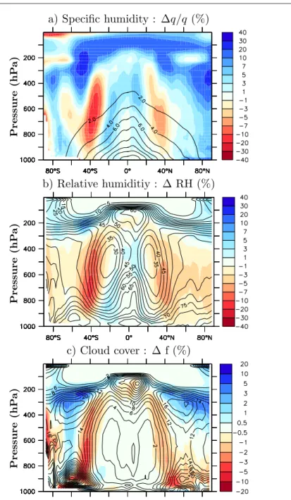
2.1 The LMDZ4 general circulation model
112
LMDZ is an atmospheric general circulation model developed at Laboratoire de
113
M´et´eorologie Dynamique. The dynamical part of the code is based on a
finite-114
difference formulation of the primitive equations of meteorology (see e. g. Sadourny
115
and Laval, 1984), discretized on a stretchable (Z of LMDZ standing for Zoom
ca-116
pability) longitude-latitude Arakawa C-grid.
117
The physical parameterizations of the LMDZ4 versions are described by
Hour-118
din et al (2006). The Morcrette (1991) scheme is used for radiative transfer. Drag
119
and lifting effects associated with the subgrid-scale orography are accounted for
120
according to Lott (1999). Turbulent transport in the planetary boundary layer is
121
treated as a vertical diffusion with an eddy diffusivity Kz depending on the
lo-122
cal Richardson number according to Laval et al (1981). Up-gradient transport of
123
heat in the convective boundary layer is ensured by adding a prescribed
counter-124
gradient term of 1 K/km to the vertical derivative of potential temperature
(Dear-125
dorff, 1966). In the case of unstable profiles, a dry convective adjustment is applied.
126
The surface boundary layer is treated according to Louis (1979). Deep convection is
127
parameterized using the ”episodic mixing and buoyancy sorting” Emanuel scheme
128
(Emanuel, 1991) which assumes quasi-equilibrium between the opposite influences
129
of the large-scale forcing of convection and of convective instability. A statistical
130
cloud scheme is used to predict the clouds properties with a different treatment
131
for convective clouds (Bony and Emanuel, 2001) and large-scale condensation as
132
explained by Hourdin et al (2006).
133
The IPSL-CM4 simulations made for CMIP3 were performed with a
configura-134
tion of LMDZ4 made of 96 points in longitude by 72 in latitude (about 3.75◦×2.5◦
)
135
and 19 layers on the vertical (Marti et al, 2010).
136
2.2 Sensitivity experiments
137
Identical changes in horizontal resolution are explored here in both imposed-SST
138
and coupled atmosphere-ocean simulations with exactly the same source code for
139
the atmospheric component LMDZ4, using a 19-layer vertical grid (L19). The
140
dynamical time-step and the time constants for the horizontal diffusion are the only
141
— necessary — parameter changes between the different simulations, as described
142
below. The other components of the system, i. e. the land surface scheme Orchidee
143
and the oceanic circulation model Nemo, are also strictly identical (those versions
144
are described by Marti et al, 2010).
145
In the imposed-SST simulations, seasonally varying SSTs are imposed as a
146
boundary condition. In practice, a climatological average of the AMIP SSTs
(Hur-147
rell et al, 2008) over the period 1970–2000 is used in order to minimize the
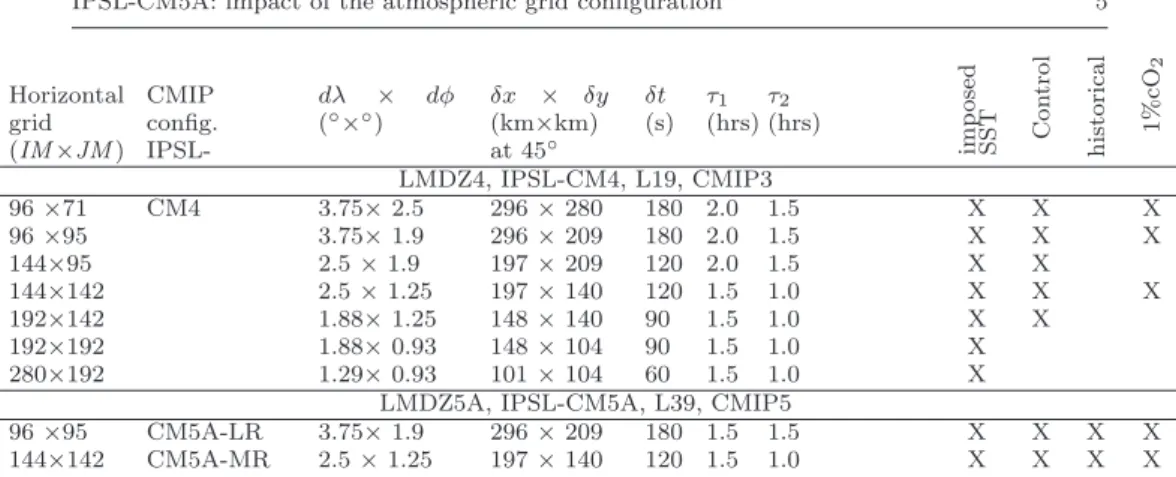
im p o sed S S T Con tr o l h ist o ri ca l 1 % cO 2 Horizontal grid (IM ×JM ) CMIP config. IPSL-dλ × dφ (◦×◦) δx × δy (km×km) at 45◦ δt (s) τ1 (hrs) τ2 (hrs) LMDZ4, IPSL-CM4, L19, CMIP3 96 ×71 CM4 3.75× 2.5 296 × 280 180 2.0 1.5 X X X 96 ×95 3.75× 1.9 296 × 209 180 2.0 1.5 X X X 144×95 2.5 × 1.9 197 × 209 120 2.0 1.5 X X 144×142 2.5 × 1.25 197 × 140 120 1.5 1.0 X X X 192×142 1.88× 1.25 148 × 140 90 1.5 1.0 X X 192×192 1.88× 0.93 148 × 104 90 1.5 1.0 X 280×192 1.29× 0.93 101 × 104 60 1.5 1.0 X
LMDZ5A, IPSL-CM5A, L39, CMIP5
96 ×95 CM5A-LR 3.75× 1.9 296 × 209 180 1.5 1.5 X X X X
144×142 CM5A-MR 2.5 × 1.25 197 × 140 120 1.5 1.0 X X X X
Table 1 Characteristics of the model configurations used for this study. The IPSL-CM4 model used for CMIP3 was based on the 96 × 71 horizontal grid configuration of the LMDZ4 atmo-spheric general circulation model with 19 layers on the vertical (L19). A series of sensitivity experiments to the horizontal grid was performed with the same model version. For CMIP5, the IPSL-CM5A model (LMDZ5A atmospheric component with 39 layers) was run both with a low resolution (LR, 96 × 95) and mid resolution (MR, 144 × 142) grid. δt is the time-step used for primitive equations integration. The physical package is called with a time-step of 30 minutes for all the model configurations. The radiative transfer is computed each two hour for the IPSL-CM4 simulations and every hour for IPSL-CM5A-LR and -MR. τ1and τ2are the
time constants for horizontal dissipation. The last four columns indicate the simulations used in the present study. See text for further explanations.
ber of years of simulation required to smooth out the inter-annual variability. The
149
forced simulations are run for 10 years.
150
For the coupled atmosphere-ocean simulations, we show results of control
sim-151
ulations in which the concentration of greenhouse gases, the Earth’s orbital
pa-152
rameters and solar irradiance, and aerosols are kept constant, with same values
153
as in the imposed-SST experiments. The model is run for 100 years. The control
154
simulations are analyzed after a spin-up phase so that the global radiative balance
155
is within 1 W/m2 from zero in all the simulations. For the illustrations bellow
156
the climatological mean seasonal cycle is computed from the last 10 years of the
157
simulations.
158
LMDZ uses for the time integration a leapfrog scheme with a Matsuno (or
159
forward/backward) step every five leapfrog time-steps. The time step δt is limited
160
by a CFL criteria, which varies linearly with the size δxmin of the smallest grid
161
cell: δt < δxmin/C, where the C constant is the external gravity waves phase speed
162
in the model. In longitude-latitude grids, the longitudinal grid size goes to zero
163
at the pole. In order to avoid the use of too small time-steps, a longitudinal filter
164
is applied to the dynamical equations after latitude φ0=60◦ in both hemispheres.
165
For a regular longitude-latitude grid as used here, the minimum scale explicitly
166
accounted for in x is δxmin= δxmax∗ cos(φ0) = δxmax/2, where δxmax= 2πa/IM
167
is the mesh size in x at the equator, a = 6400 km being the Earth radius and
168
IMthe number of grid cells in the longitudinal direction. Poleward of the latitude
169
φ0, meteorological fields are filtered so as to retain only wave lengths longer than
170
δxmin. The grid mesh size in latitude δy = πa/JM – where JM is the number of
171
points in latitude – is a constant for a given grid. Finally, the time step is limited
172
by δt < (πa/C) min(1/IM, 1/JM ).
In a longitude-latitude grid, the isotropy of the horizontal grid (δy = δx) cannot
174
be insured everywhere. The original grid, (IM, JM) = (96, 72), or (dλ, dφ)=(3.75◦,2.5◦),
175
has a ratio IM/JM = 4/3 chosen so that the grid is isotropic at close to 45◦
lat-176
itude. This choice yields δx = 3δy/2 at the equator; and the time step is limited
177
by δx at φ0. Keeping both the same resolution in longitude and the same value of
178
φ0= 60◦, it is possible to refine further the resolution in latitude up to JM = IM
179
without reducing the time step. The grid is then isotropic at 60◦ latitude, and
180
δx/δy = 2 at the equator.
181
The simulations presented here were performed with either JM = 3/4× IM or
182
JM= IM. Resolutions from (dλ, dφ)=(3.75◦,2.5◦) to (1.875◦,1.26◦) or (IM, JM)=(96,71)
183
to (192,142) were explored with the coupled atmosphere-ocean model, by
increas-184
ing successively either the latitudinal or longitudinal resolution. The same
resolu-185
tions as well as finer grids were explored with the imposed-SST model.
Character-186
istics of the simulations are given in Tab. 1.
187
In addition to the choice of a small enough time step, the numerical stability
188
of the model is ensured by the ”horizontal dissipation” operators. Those
opera-189
tors account for the interaction between the explicit and sub-grid scales. They
190
are also crucial for numerical stability. Without dissipation, the enstrophy cascade
191
— well represented in LMDZ which favors numerical conservation of enstrophy
192
(Sadourny, 1975) — would accumulate at the cut-off scale. The efficiency of those
193
operators is controlled by two constants: the number of iterationsN and a time
194
constant τ . The larger the value of N , the more scale-selective the operator is,
195
the e-folding time of an oscillation of wavenumber k scaling with k2N. The time
196
constant τ is the e-folding time of the largest value of k encountered in the mesh
197
(kmax ∼ 1/δxmin). In practice, a Laplacian operator is used for the lateral
diffu-198
sion of potential temperature, while the vector Laplacian used for wind dissipation
199
is divided into rotational and divergent components.N = 2 is used for the
tem-200
perature and the wind rotational, with the same time constant τ1. For the wind
201
divergence, a stronger dissipation is applied by using bothN =1 and a shorter time
202
constant τ2 < τ1. In practice, the time constants are slightly adjusted (reduced)
203
empirically to insure numerical stability when refining the grid. Note however that
204
the effective diffusivity at a given scale decreases drastically when refining the grid.
205
The retained values are given in Tab. 1.
206
2.3 SST cold biases and dynamical structure
207
One of the major deficiencies of the IPSL-CM4 CMIP3 simulations was a strong
208
cold bias in the mid-latitude SSTs, in both the Northern and Southern hemispheres
209
(Swingedouw et al, 2007; Marti et al, 2010). The zonal-mean bias reaches 4 K
210
around 40◦of latitude for the IPSL-CM4 96× 71 simulation (Fig. 1). Refining the
211
resolution in latitude significantly reduces this bias. With a refinement in longitude,
212
the warming of the model is essentially located in the tropics, as illustrated further
213
in Fig. 2. The equator-to-mid-latitude surface temperature contrast is generally
214
0.5-1 K smaller (and thus closer to observations) when the same number of points
215
is used in longitude and latitude. The bias in the equator-to-mid-latitude contrast
216
is of 4 K for the 96×71 simulation, which has nearly zero SST-bias at the equator.
217
It reduces down to 2 K in the 144× 142 case, but increases back to 3 K for the
218
192× 142 grid.
✲✁ ✲✂ ✁ ✲ ✄✁ ✁ ✄✁ ✂ ✁ ✁ ▲☎ ✆✝✆✞ ✟ ✠ ✲✡ ✲☛ ✁ ☛ ✡ ❚ ☞ ✌ ✍ ☞ ✎ ✏ ✑ ✒ ✎ ☞ ✓ ✔ ✏ ✕ ✖ ✗ ✘ ❈ ✙✡ ✲✂ ✚ ✛ ✜ ❈ ✙✡ ✲✂ ✚ ✢ ❈ ✙✡ ✲ ✜✡ ✡✚ ✢ ❈ ✙✡ ✲ ✜✡ ✡✚ ✜✡ ☛ ❈ ✙✡ ✲ ✜☛✚ ✜✡ ☛
Fig. 1 Biases in SST (K) for the various configurations of the IPSL-CM4 model. The biases are computed with respect to the Levitus climatology, and zonally averaged. We analyze the last 10 years of 100-year simulations starting from the same oceanic state. The red curves correspond to cases where IM = JM .
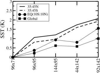
✾ ✁ ✂ ✄ ✾ ✁ ✾ ☎ ✄ ✶ ✶ ✁ ✾ ☎ ✄ ✶ ✶ ✁ ✄ ✶ ✆ ✄ ✾ ✆ ✁ ✄ ✶ ✆ ✵ ✵✝✞ ✟ ✟✝✞ ✷ ✷✝✞ ✸ ❙ ❙ ✠ ✡ ☛ ☞ ✌ ✍ ✎✏✍ ✑ ✌ ✍ ✎✏✍ ✒ ❊ ✓✔ ✕ ✖✒ ✎✕✖✑✗ ● ✘✙✚ ✛✘
Fig. 2 Evolution with the model horizontal resolution of the SST (K) for the global average (squares), for the southern (45-35S, dashed line) and northern (35-45N, full line) mid-latitudes and for the Equator (5S-5N, circles). The values from the coarsest grid (96×71) are subtracted.
The reduction of the cold bias of the mid-latitudes when refining the grid is
220
accompanied by a poleward shift of the mid-latitude jets (Fig. 3). This shift is
221
present both in the IPSL-CM4 coupled and LMDZ4 imposed-SST simulations. It
222
corresponds to a strong reduction of the biases in the representation of the mean
223
zonal wind with grid refinement, as illustrated in the left column of Fig. 4 for the
224
imposed-SST simulations. For the coarsest grids, the jets are shifted toward the
225
equator compared to ERA interim reanalyzes (as seen from the strong dipole in
226
the zonal wind bias, centered at the latitude of the jet maximum intensity).
227
This jet displacement was studied by Guemas and Codron (2011) in a set of
228
dynamical core experiments produced with the LMDZ atmospheric model using
229
the Held and Suarez (1994) setup. This setup consists in replacing all the detailed
230
physical parameterizations by a Newtonian relaxation of the temperature field
✾ ✁ ✂ ✄ ✾ ✁ ✾ ☎ ✄ ✶ ✶ ✁ ✾ ☎ ✄ ✶ ✶ ✁ ✄ ✶ ✆ ✄ ✾ ✆ ✁ ✄ ✶ ✆ ✄ ✾ ✆ ✁ ✄ ✾ ✆ ✆ ✷ ✝ ✁ ✄ ✾ ✆ ✵ ✞ ✟ ✸ ✹ ✺ ✻ ✼ ❏ ✠ ✡ ☛ ☞ ✡ ✌ ✡ ✍ ✎ ✠ ✏ ✥ ✮ ▲ ✑✒ ✓✔✕✖✗✘✙ ✚ ▲ ✑✒ ✓✔✕✛✗✜✙ ✚ ■✢ ✛▲ ✕✣✑ ✔✕✖✗✘✙✚ ■✢ ✛▲ ✕✣✑ ✔✕✛✗✜✙✚
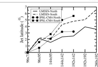
Fig. 3 Latitude of the mid-latitude jets, computed at the 850hPa level, for the two hemispheres and for the imposed-SST (LMDZ4) and coupled atmosphere-ocean (IPSL-CM4) simulations. The latitude is counted positive from equator to pole in both hemispheres and the values from the coarsest (96 × 71) grid are subtracted.
toward a zonally-symmetric state, and a Rayleigh (linear) damping of the low-level
232
wind with an e-folding timescale of 1 day at the surface. In this configuration, it
233
was shown that the jet latitude moves poleward when refining the grid in latitude,
234
and is less affected when increasing the number of grid points in longitude. It was
235
checked also in this idealized framework that the changes in jet location when
236
refining the grid do not come from the use of a shorter time-step.
237
A similar behavior is found for the imposed-SST and coupled climate
simula-238
tions shown here (Fig. 3): a tendency of the jets to move toward the poles when
239
increasing the resolution, with a stronger impact when refining the grid in latitude.
240
The effect is not as systematic as in the idealized dynamical simulations of Guemas
241
and Codron (2011), which may reflect additional effects due to the complexity of
242
the climate system.
243
In order to understand how the grid refinement impacts the SSTs, i. e. both
244
the increase of the mean temperature and reduction of the latitudinal contrasts,
245
we start by analyzing the change in thermodynamical variables and energy budget
246
in the imposed-SST simulations.
247
2.4 Thermodynamical variables in the imposed-SST simulations
248
The changes in zonal winds shown in Fig. 4 are accompanied by systematic changes
249
in the temperature and humidity fields.
250
The mid-latitude tropopause (close to 200 hPa) moistens when refining the
251
horizontal grid, and becomes too moist when compared to ERA-Interim for the
252
finest grids. The tropopause cold bias of the mid to high latitudes also increases.
253
These two trends are probably related to each other since the cooling to space,
254
a dominant term of the radiative balance at this level, is strongly affected by
U (m/s) T (◦C) RH (%) L M D Z 4 :9 6 × 7 1 Pr e s s ur e ( hP a ) L M D Z 4 :9 6 × 9 5 Pr e s s ur e ( hP a ) L M D Z 4 :1 4 4 × 9 5 Pr e s s ur e ( hP a ) L M D Z 4 :1 4 4 × 1 4 2 Pr es s ur e ( hP a ) L M D Z 4 :1 9 2 × 1 4 2 Pr es s ur e ( hP a ) L M D Z 4 :2 8 0 × 1 9 2 Pr es s ur e ( hP a )
Fig. 4 Ten-year average of the mean meridional structure of the zonal wind (m/s, left), tem-perature (◦C, middle) and relative humidity (%, right) for the various imposed-SST simulations with LMDZ4 (L19). The contours correspond to the simulations and the colors to the difference (bias) with ERAinterim re-analayzes.
humidity as already discussed by Hourdin et al (2006). Overall, the mid-latitude
256
tropopause is thus too high for the finest grids explored.
257
The systematic dry bias of the tropical boundary layer top (900 hPa) is a
258
direct consequence of an underestimated moisture vertical transport by the
eddy-259
diffusion parameterization used in LMDZ4. It is therefore not affected by the
260
changes in horizontal resolution.
261
Grid refinement leads to a systematic decrease of the wet and cold bias of the
262
mid-latitude troposphere. This decrease of relative humidity is not just a
conse-263
quence of the warmer temperature since the specific humidity is reduced as well,
264
as illustrated in Fig. 5a and b that show differences between the 96× 71 and
265
144× 142 grids. These changes can be interpreted as a shift toward the poles of
266
the dry anticyclonic regions of the sub-tropics, as seen from the coincidence of the
267
location of the maximum drying with that of the maximum latitudinal gradient
268
of relative humidity (Fig. 5b).
269
The impact of the poleward displacement of the jet and of the Hadley-cell
270
boundary is also apparent in the water budget. The difference of integrated
merid-271
ional transport of moisture between the 144× 142 and 96 × 71 resolutions is shown
272
on Fig. 6a (the transport of Lq is shown here where L is the specific latent heat
273
and q the specific humidity). The Hadley circulation transports water toward the
274
equator (more water being transported in the lower branch of the cell), while the
275
Ferrel Cell and mid-latitude eddies transport moisture toward the pole. A wider
276
Hadley cell will thus increase the equatorward transport near the latitudinal edge
277
of the cell, while the displacement of the mid-latitude eddies will increase poleward
278
transport in higher latitudes. The differential transport with increased resolution
279
is therefore systematically away from the mid-latitudes (40◦N and 40◦S) towards
280
the equator and poles. As a consequence, precipitation is reduced in the
mid-281
latitudes (Fig. 6b), even though the evaporation increases weakly because of the
282
drier atmosphere.
283
2.5 Energy budget in the imposed-SST simulations
284
The changes in relative humidity illustrated in Fig. 5b between resolutions 96× 71
285
and 144× 142 coincide with large changes in cloud fraction (Fig. 5c).
Specifi-286
cally, the cloud fraction exhibits a significant decrease near 40◦ latitude in both
287
hemispheres, and a systematic increase at the tropopause.
288
The changes in clouds are associated with pronounced changes in the
Top-289
of-Atmosphere (TOA) radiative budget (Fig. 6d). The short-wave (SW)
Cloud-290
Radiative-Forcing (CRF), defined as the difference of the TOA SW radiation
be-291
tween all-sky and clear-sky conditions, is strongly increased in the mid-latitudes,
292
as a consequence of the decrease of the fractional coverage of low and mid-level
293
clouds. For long-wave (LW) radiation, the effect of clouds and the modification
294
of clear-sky radiation partially cancel each other. The change in SW CRF does
295
not affect significantly the atmospheric budget (red curve in Fig. 6c), since the
in-296
crease of down-welling SW radiation at surface (red curve in Fig. 6e) is very close
297
to that at TOA. Conversely, the decrease in low-level cloud cover and near surface
298
humidity in the mid latitudes reduces the LW radiation of the atmosphere toward
299
the surface (green dashed curve in Fig. 6e). The change of net LW radiation (full
300
green curve) is almost identical to the change in downweling LW radiation except
a) Specific humidity : ∆q/q (%)
Pr e ss u re (h P a )b) Relative humiditiy : ∆ RH (%)
Pr e ss u re (h P a )c) Cloud cover : ∆ f (%)
Pr e ss u re (h P a )Fig. 5 Zonal mean change of the latitude-pressure distribution of moisture and clouds in LMDZ4 imposed-SST simulations associated with grid refinement from 96 × 71 to 144 × 142: a) relative difference in specific humidity (%), b) difference in relative humidity (%) and c) difference in cloud fraction (%). The differences are in color while the contours correspond to the mean value of the 144 × 142 simulation (resp. in g/kg, % and %).
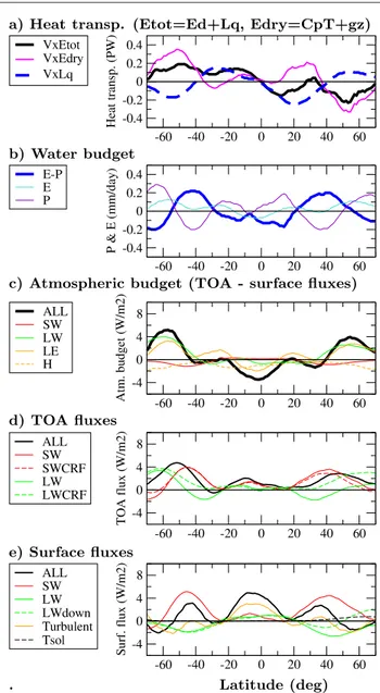
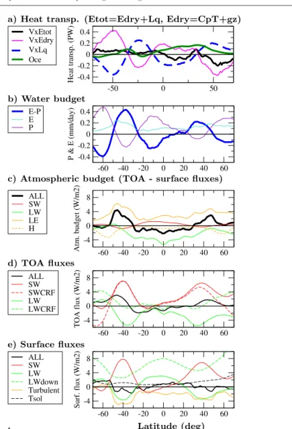
a) Heat transp. (Etot=Ed+Lq, Edry=CpT+gz) ✲ ✁✂ ✲ ✁✄ ✁✄ ✁✂ ❍ ☎ ✆ ✝ ✝ ✞ ✆ ✟ ✠ ✡ ☛ ☞ ✌ ✍ ✎ ✲✏ ✲ ✂ ✲✄ ✄ ✂ ✏ ❱✑✒✓✔✓ ❱✑✒✕✖ ✗ ❱✑✘✙ b) Water budget ✚✛ ✜✢ ✚✛ ✜✣ ✛ ✛ ✜✣ ✛ ✜✢ P ✤ ✥ ✦ ✧ ✧ ★ ✩ ✪ ✫ ✬ ✚✭✛ ✚ ✢✛ ✚ ✣✛ ✛ ✣ ✛ ✢ ✛ ✭✛ ❊✚ ✮ ❊ ✮
c) Atmospheric budget (TOA - surface fluxes)
✯✰ ✵ ✰ ✽ ❆ ✱ ✳ ✴ ✶ ✷ ✸ ✹ ✺ ✱ ✻ ✼ ✾ ✳ ✿ ❀ ✯❁✵ ✯ ✰✵ ✯❂✵ ✵ ❂✵ ✰✵ ❁✵ ❃❄❄ ❙❅ ❄❅ ❄▲ ❇ d) TOA fluxes ❈❉ ❋ ❉ ● ❚ ■ ❏ ❑ ▼ ◆ ❖ ◗ ❘ ❯ ❲ ❳ ❨ ❈❩❋ ❈ ❉❋ ❈❬❋ ❋ ❬❋ ❉❋ ❩❋ ❭❪❪ ❫ ❴ ❫ ❴❵❛ ❜ ❪❴ ❪❴❵❛❜ e) Surface fluxes ❝❞ ❡ ❞ ❢ ❣ ❤ ✐ ❥ ❦ ❥ ❧ ❤ ♠ ♥ ♦ ♣ q r s ❝t❡ ❝ ❞❡ ❝✉❡ ❡ ✉❡ ❞❡ t❡ ✈✇✇ ① ② ✇② ✇②③④ ⑤⑥ ⑦ ⑧⑨⑩ ⑧❶❷⑥❸ ⑦❹④❶ . Latitude (deg)
Fig. 6 Change in atmospheric transport, water and energy budget between the 96×71 LMDZ4 imposed SST simulation and the 144 × 142 configuration : a) change in meridional energy transport (in PW), the moist static energy Etot being decomposed into its dry component CpT + gz and latent heat Lq; b) change in evaporation (E), precipitation (P ) and water
budget (E − P ) ; c) change in atmospheric budget, difference between the TOA and surface (downward) fluxes, separating the contribution of SW and LW radiation, and the latent (LE) and sensible (H) heat flux at surface ; d) TOA fluxes, for LW and SW radiation together with the corresponding CRF ; e) surface downward fluxes. For the LW radiation, we show in green both the net radiation (full line) and down-welling radiation (dashed). The changes in turbulent flux −(H + LE) and mean surface temperature are also shown in e (orange and dashed black curves respectively). In c, d and e, ALL means the sum of the LW, SW and turbulent contributions. Note that a 20-degree area conserving running mean is applied in latitude to all the fields in order to remove the numerical noise that results from differences computed between two different grids.
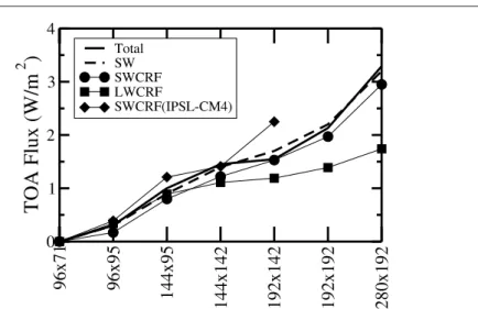
✾ ✁ ✂ ✄ ✾ ✁ ✾ ☎ ✄ ✶ ✶ ✁ ✾ ☎ ✄ ✶ ✶ ✁ ✄ ✶ ✆ ✄ ✾ ✆ ✁ ✄ ✶ ✆ ✄ ✾ ✆ ✁ ✄ ✾ ✆ ✆ ✷ ✝ ✁ ✄ ✾ ✆ ✵ ✞ ✟ ✸ ✹ ❚ ✠ ✡ ☛ ☞ ✌ ✍ ✎ ✏ ✑ ✒ ✥ ✮ ✓ ✔✕ ✖✗ ❙ ✘ ❙ ✘✙✚✛ ▲✘✙✚✛ ❙ ✘✙✚✛✜✢✣❙▲✤✙✦ ✧★
Fig. 7 Impact of the grid resolution on the top-of-atmosphere (TOA) fluxes (W/m2) in the
imposed-SST LMDZ4 simulations. The total (LW+SW) net radiation (full curve) together with the SW component (dashed), SW CRF (circles) and LW CRF (squares) are shown. Results from the 96×71 simulation are subtracted. The SW CRF of the coupled IPSL-CM4 simulations (diamonds) is also shown for comparison. All the diagnostics correspond to 10-year means.
in the northern mid and high latitudes where continental surfaces respond to the
302
increased surface incoming SW radiation.
303
The sensible heat flux is reduced rather systematically by about 1 W/m2due to
304
the warmer atmosphere. The latent heat is reinforced in the mid latitudes but with
305
a local minimum at 40 degrees latitude. All together, the atmosphere is heated by
306
diabatic processes in the mid-latitudes more than in the tropics, which induces a
307
reduction of the total latitudinal energy transport (black curve in Fig. 6a). This
308
decrease is however weak, with a partial compensation between the transport of
309
Lq and that of the dry static energy CpT + gz.
310
In the imposed-SST LMDZ4 simulations, the global value of the total longwave
311
plus shortwave (LW+SW) radiation at TOA (full curve in Fig. 7) systematically
312
increases with grid refinement. It changes by +3 W/m2 (a gain for the climate
313
system) when going from the coarsest to the finest grid. For the global average,
314
this additional heat for the climate system can be entirely explained by the change
315
in SW CRF, associated with a reduction of the averaged low-level cloud cover from
316
almost 27% for the 96× 71 grid to less than 24% for the finest 280 × 192 grid. The
317
LW CRF also increases with grid refinement but is compensated by a decrease of
318
the clear-sky Outgoing Longwave Radiation (OLR, not shown), so that the total
319
OLR is almost independent of grid resolution (as evidenced by the fact that the
320
total and SW radiation almost coincide in Fig. 7).
321
We detail below the specific modifications of the SW CRF that result from a
322
grid refinement in either longitude or latitude. Refining the grid in latitude induces
323
a maximum of SW CRF increase in the mid-latitudes (red curve in Fig. 8a) which
324
may be explained by the latitudinal shift of the jets: the jets being closer to the
325
pole in the finest grids, the region of strong (negative) SW CRF associated with the
326
storm-tracks is shifted towards latitudes where the insolation is weaker, resulting
327
in a weaker SW CRF and also in a weaker low-level cloud cover. because of the
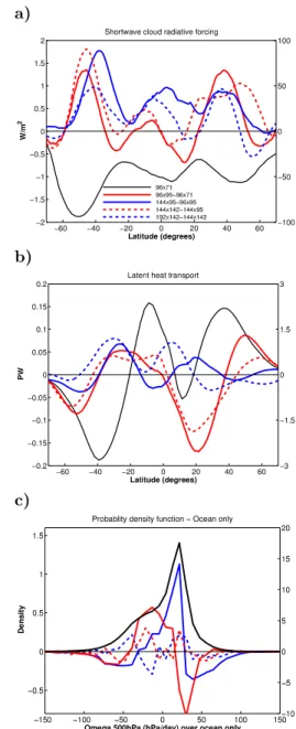
a) ✲✁ ✲✂✁ ✲✄✁ ✁ ✄✁ ✂✁ ✁ ✲✄ ✲☎✆✝ ✲☎ ✲✁✆✝ ✁ ✁✆✝ ☎ ☎✆✝ ✄ ✥ ✞✟✠ ✟✡☛☞✌☛ ☞✍ ✎☞☞✏✑ ✒ ✓ ✔ ✷ ❙✕✖✗✘✙ ✚✛✜✢✣✖✤✦✗✚✦✧✚✘✧ ✛✜★✖ ✗ ✢✧ ✩✪ ✾ ✫✬ ✭ ✮ ✾ ✫✬ ✾ ✯✰ ✾✫✬✭✮ ✮✶ ✶✬ ✾ ✯✰ ✾ ✫✬ ✾ ✯ ✮✶ ✶✬ ✮✶✱✰ ✮✶✶✬✾✯ ✮ ✾✱ ✬ ✮✶✱✰ ✮✶✶✬✮✶✱ ✲☎✁✁ ✲✝✁ ✁ ✝✁ ☎✁✁ b) ✳✴✵ ✳ ✸✵ ✳ ✹✵ ✵ ✹✵ ✸✵ ✴✵ ✳✵✺✹ ✳✵✺✻✼ ✳✵✺✻ ✳✵✺✵✼ ✵ ✵✺✵✼ ✵✺✻ ✵✺✻✼ ✵✺✹ ✽✿❀ ❁❀ ❂❃ ❄❅❃ ❄❆❇ ❄❄❈❉ ❊ ❋ ▲●❍■❏❍❑ ■●❍❍▼ ●❏◆❖P ▼❍ ✳◗ ✳✻✺✼ ✵ ✻✺✼ ◗ c) ❘ ❚❯ ❱ ❘ ❚ ❱❱ ❘ ❯ ❱ ❱ ❯❱ ❚ ❱❱ ❚❯ ❱ ❘ ❱❲❯ ❱ ❱❲❯ ❚ ❚❲❯ ❳❨ ❩❬❭❪❫❫ ❴❵ ❭❛❴❵ ❭ ❜❝❭ ❞❡❢❣ ❩❤❢✐ ❩❭ ❥❢ ❥❦ ❞ ❧ ♠ ♥ ♦ ♣ q r s t ✉✈ ✇✈ ①② ③④⑤⑥ ⑦⑧ ② ③④⑨⑩ ⑦❶ ③② ✉ ⑦❘❷❶ ⑥✇⑦✉⑦ ①④ ❘ ❚❱ ❘ ❯ ❱ ❯ ❚❱ ❚❯ ❸ ❱
Fig. 8 Impact of grid refinement on: a) the latitudinal distribution of the SW CRF, b) the meridional transport of latent heat (Lq), and c) the PDF (Probability Density Function) of the 500 hPa large-scale vertical velocity ω500 in the Tropics (30◦S-30◦N). The red (respectively
blue) curves show the difference between pairs of imposed-SST experiments with consecutive grid refinement in latitude (respectively in longitude). Scales are on the left vertical axis. For each graph, the black curve corresponds to the simulation with the 96 × 71 grid. The corresponding values are on the right vertical axis.
wider meridional extent of the trades. Consistently, the grid refinement in latitude
329
has a clear effect on the meridional water transport with a systematically increased
330
transport away from the mid-latitudes, towards both the poles and the equator
331
(red curves in Fig. 8b).
332
When increasing the resolution in longitude, the effect on the SW CRF is
333
stronger in the tropics (blue curves in Fig. 8a), and is less clearly related to a
334
change in the meridional moisture transport. This can be related to changes in the
335
PDF (Probability Density Function) of the 500 hPa large-scale vertical velocity,
336
ω500, that characterizes the large-scale tropical circulation (Bony et al, 2004). The
337
change in tropical dynamics is particularly clear when increasing the resolution in
338
longitude from 96× 95 to 144 × 95 (full blue curve in Fig. 8c). The deep convective
339
regimes (ω500<-40 hPa/day) associated with the ITCZ and the strong subsiding
340
regimes (ω500 >30 hPa/day) associated with strato-cumulus regions both have a
341
strongly reduced occurrence, with a compensating increase in the weakly subsiding
342
regimes. These two extreme regimes correspond to maximum cloud coverage and
343
SW CRF, so their diminution could partly explain the reduction of the SW CRF
344
in the tropics, which was particularly large for this change of resolution. When
345
increasing the resolution in latitude from 96× 71 to 96 × 95 (red curve in Fig. 8c)
346
the change of the PDF is dominated by a transfer from the weakly subsiding to the
347
weakly ascending regimes so that the ascending motions are globally reinforced on
348
the domain retained for analysis (the ocean in the 30◦S-30◦N latitude band). This
349
increased ascent is compensated by subsidence in the extra-tropics. These changes
350
are accompanied in this particular case by a slight decrease of the SW CRF in the
351
tropics (Fig. 8). The effects of resolution changes are weaker when exploring finer
352
resolutions, in terms of both PDF and SW CRF changes.
353
2.6 Impact on SST in the coupled experiments
354
The changes with resolution of the global SW CRF are quite similar in the coupled
355
(Fig. 9) and imposed-SST simulations (the SW CRF of the coupled simulations is
356
duplicated in Fig. 7 for comparison). The latitudinal distribution of these changes
357
of SW CRF are also quite similar, as can be seen for resolutions 96× 71 and
358
144× 142 by comparing the dashed red curves in Fig. 6d and Fig. 10d.
359
In the coupled IPSL-CM4 simulations, the imbalance of the TOA radiative
360
budget associated with grid refinement, coming from the change in SW CRF, acts
361
as an initial forcing and induces a warming of the global surface temperature until
362
a new equilibrium is reached. After 90 years, the total net flux in the simulations
363
shown here is close to zero, as expected for an equilibrated coupled simulation. The
364
total flux is of -0.4 W/m2 for the 96× 71 grid. The other resolutions have a total
365
balance less negative by a fraction of a W/m2(full curve in Fig. 9), indicating that
366
the various simulations are not too far from radiative equilibrium. Note that there
367
is an energy leakage of the order of 0.2 W/m2in all the coupled atmosphere-ocean
368
simulations presented here (see Dufresne et al., this issue).
369
The direct forcing induced by the SW CRF change on the temperature is then
370
amplified by classical climate feedbacks resulting from the surface temperature
371
increase. This can be illustrated from the comparison of the 96× 71 and 192 × 142
372
simulations, i. e. focusing on the values associated with grid 192× 142 on the
373
x-axis in Fig. 7 and 9. Simulations with imposed SST show that the initial SW
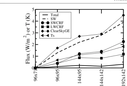
✾ ✁ ✂ ✄ ✾ ✁ ✾ ☎ ✄ ✶ ✶ ✁ ✾ ☎ ✄ ✶ ✶ ✁ ✄ ✶ ✆ ✄ ✾ ✆ ✁ ✄ ✶ ✆ ✵ ✝ ✷ ✸ ✹ ✺ ❋ ✞ ✟ ✠ ✡ ☛ ☞ ✌ ✥ ✮ ✍ ✎ ✏ ✡ ✑ ✮ ❚✒✓✔ ✕ ❙✖ ❙✖✗✘✙ ▲✖✗✘✙ ✗✕❈✔✚❙✛✜✢ ✣ ❚✤
Fig. 9 Impact of the grid resolution on the TOA fluxes (W/m2) and global-mean surface
temperature Ts (triangles, in K) in the coupled atmosphere-ocean IPSL-CM4 simulations.
Results from the 96 × 71 simulation are subtracted. The total (LW+SW) net radiation (full curve) together with the SW component (dashed), SW CRF (circles), LW CRF (squares), clear sky greenhouse term (diamonds) are shown. All the diagnostics correspond to 10-year means.
CRF between the two resolution is 1.5 W/m2 (circles in Fig. 7). The SW-CRF
375
is reinforced by about 0.7 W/2 in the coupled experiments (positive feedback,
376
as seen by comparing circles and diamonds in Fig. 7). The difference between
377
the absorbed solar radiation (SW) and the SW CRF in Fig. 9 reflects a positive
378
feedback from the surface albedo (of about 1.7 W/m2), resulting from a decrease
379
in snow and ice cover. Between the forced and coupled simulation the role of clouds
380
on longwave radiation remains comparable (squares in Fig. 7 and 9). The change
381
in TOA SW radiation is around 4 W/m2 and so is the change in OLR in the
382
coupled simulations.
383
The change in LW emission by the surface, σTs4, can be formally decomposed
384
as the sum of the change in OLR and in Greenhouse Effect (GE) term (Raval and
385
Ramanathan, 1989)
386
GE = σTs4− OLR (1)
with a strong contribution of the clear-sky GE (diamonds in Fig. 9) associated with
387
water vapor and lapse rate feedbacks. Finally, a temperature increase of 1.8 K is
388
obtained for an initial SW CRF of 1.5 K in the imposed-SST simulations. The
389
sensitivity close to 1.2 K per W/m2, obtained here from a change in horizontal
390
grid, is comparable to that obtained in climate change simulations with the
IPSL-391
CM4 model.
392
In terms of modification of the latitudinal structures, the results also follow
393
what was observed in imposed-SSTs simulations, but for the above mentioned
394
feedbacks. As was the case in the imposed-SSTs simulations, the atmospheric
395
transport tends to dry the mid latitudes (Fig. 10a and b). The TOA SW CRF
396
shows, similarly, a maximum increase in the mid latitudes. The surface albedo
397
feedback is seen by the fact that the change in total TOA SW radiation (full red
398
curve in Fig. 10d) in the high latitudes is somewhat larger than the CRF (dashed)
a) Heat transp. (Etot=Edry+Lq, Edry=CpT+gz) ✲ ✁ ✂ ✲ ✁✄ ✁✄ ✁ ✂ ❍ ☎ ✆ ✝ ✝ ✞ ✆ ✟ ✠ ✡ ☛ ☞ ✌ ✍ ✎ ✲✏ ✏ ❱ ✑✒✓✔✓ ❱ ✑✒✕ ✖✗ ❱ ✑✘✙ ❖ ✚✛ b) Water budget ✜✢ ✣✤ ✜✢ ✣✥ ✢ ✢ ✣✥ ✢ ✣✤ P ✦ ✧ ★ ✩ ✩ ✪ ✫ ✬ ✭ ✮ ✜✯✢ ✜ ✤✢ ✜✥✢ ✢ ✥✢ ✤ ✢ ✯✢ ❊✜✰ ❊ ✰
c) Atmospheric budget (TOA - surface fluxes)
✱✳ ✵ ✳ ✽ ❆ ✴ ✶ ✷ ✸ ✹ ✺ ✻ ✼ ✴ ✾ ✿ ❀ ✶ ❁ ❂ ✱❃✵ ✱ ✳✵ ✱❄✵ ✵ ❄ ✵ ✳✵ ❃✵ ❅❇❇ ❙❈ ❇❈ ❇▲ ❉ d) TOA fluxes ❋● ■ ● ❏ ❚ ❑ ▼ ◆ ◗ ❘ ❯ ❲ ❳ ❨ ❩ ❬ ❭ ❋❪■ ❋ ●■ ❋❫■ ■ ❫■ ●■ ❪■ ❴❵❵ ❛ ❜ ❛ ❜❝❞ ❡ ❵❜ ❵❜❝❞❡ e) Surface fluxes ❢❣ ❤ ❣ ✐ ❥ ❦ ❧ ♠ ♥ ♠ ♦ ❦ ♣ q r s t ✉ ✈ ❢✇❤ ❢ ❣❤ ❢①❤ ❤ ① ❤ ❣❤ ✇❤ ②③③ ④ ⑤ ③⑤ ③⑤ ⑥⑦ ⑧⑨ ⑩ ❶❷❸ ❶❹❺⑨❻ ⑩❼⑦❹ . Latitude (deg)
Fig. 10 Same as Fig. 6 but for the coupled IPSL-CM4 simulations. The change in oceanic heat transport is added on panel a) (thick green curve).
while the two curves were almost superimposed in the imposed SST simulations
400
(Fig. 6d). The coupled atmosphere-ocean system tends to re-adjust to this SW
401
forcing, so that, at the end, the increased OLR in the mid latitudes almost
com-402
pensates for the increased SW radiation (green and red full curves of Fig. 10d).
403
The surface temperature increase (black dashed curve in Fig. 10e) is somewhat
404
larger in the mid- and high-latitudes than at the equator so that the turbulent
405
fluxes (latent + sensible) tend to increase specifically at those latitudes (an
heat-406
ing for the atmosphere). The new equilibrium in the coupled model also results in
407
a reduction of the atmospheric equator to pole heat transport (Fig. 10a). However
✾ ✁ ✂ ✄ ✾ ✁ ✾ ☎ ✄ ✶ ✶ ✁ ✾ ✄ ✶ ✶ ✁ ✄ ✶ ✆ ✄ ✾ ✆ ✁ ✄ ✶ ✆ ✽ ✝ ✞ ✝ ✝ ✞✟✝ ✞ ✠ ✝ ✞ ✡ ✝ ✞ ✽ ✝ ✟✝ ✝ ❉ ☛ ☞ ✌ ✍ ✎ ☛ ☞ ✏ ✑ ✒ ✓ ☛ ✎ ✔ ✕ ✖ ✗ ☞ ✏ ✘ ✙ ✚ ✛ ✜ ✏ ✖ ✍ ✏ ✎ ✓ ☛ ✢ ✔ ✣ ✤ ✓ ✥ ✗ ✦✧★ ✩✪✫✧★ ✬✭ ✮✯✧ ✫✰✱✲✳ ✴ ✵✷✸✹ ✦✧★ ✩✪✫✧★ ✬✭ ✮✯✧ ✫✰ ✺✻✳✼✿✯❀★ ✬❁❂❃ ❄❂ ❅ ◆✺❆❃✬❇✪✬ ✫ ✯✧❈✼ ❊❋✳✵●●✳❍❋✵■❋❋❏ ❅✰✱✲✳ ✴ ✵✷✸✹ ◆✺❆❃✬❇✪✬ ✫ ✯✧❈✼ ❊❋✳✵●●✳❍❋✵■❋❋❏ ❅✰✺✻✳
Fig. 11 Volume transport through Drake Passage (between the southern tip of America and Antarctica), in black, and nitrate inventories in the Southern Ocean (90S-55S, 0m-200m), in red. Circles are for the IPSL-CM4 simulations with various horizontal grids. Data (dashed lines) correspond to Cunningham et al (2003) for the Drake transport and Conkright et al (2002) for nitrate inventories. Note that the PISCES biogeochemical model has been run offline for the results shown here, with the same ocean grid configuration for all the atmospheric grids.
the magnitude is smaller than in the atmosphere alone simulations, mainly because
409
the warmer SSTs lead to enhanced evaporation with resolution that
counterbal-410
ances the surface net radiation, which smoothes the changes in the atmospheric
411
equator to pole energy budget compared to the imposed-SST simulations.
412
2.7 Oceanic transport
413
The poleward shift of the jets has a positive impact on the ocean gyre circulation
414
in the north Atlantic (illustrations not shown). The warm and saltier water from
415
the tropics are advected further north in the Atlantic, which reinforces deep water
416
formation and the northward heat transport by the ocean circulation by up to
417
0.15 PW at 30◦N between the coarsest (96× 71) and finest (144 × 142) grid.
418
The processes involved are similar to the one discussed by Marti et al (2010).
419
The role of the Atlantic in the northern hemisphere is directly reflected on the
420
changes in the global heat transport by the ocean circulation (thick green curve in
421
Fig. 10a). These changes in the ocean circulation partially counteract the reduction
422
of the heat transport by the atmospheric circulation discussed above. However the
423
changes in the atmosphere of about 0.2 PW between the coarsest and finest grid
424
considered here are larger than those of the ocean so that the sum of the heat
425
transport by the ocean and the atmosphere reduces with resolution, reflecting the
426
dominant role of the readjustments of temperature, humidity and clouds in the
427
atmospheric column on the new equilibrium.
428
The southward shift and intensification of the westerlies associated with the
429
poleward shift of the atmospheric mid-latitude jets with resolution increase the
430
mass flux of the Antarctic Circumpolar Current, as shown by the volume
port through Drake Passage (Fig. 11). These changes have a positive impact on
432
the representation of the nutrient fields in the ocean. It can be inferred from
sim-433
ulations performed with the PISCES biogeochemical model (Aumont and Bopp,
434
2006) forced by the CM4 ocean circulation. We focus here on the first 200 m
ni-435
trate inventories in the Southern Ocean (south of 55◦S). These inventories are key
436
in setting the Southern Ocean biological productivity, and also in determining the
437
nutrient concentrations of the tropical oceans (Sarmiento et al, 2004). The suite
438
of CM4 simulations clearly shows that changes in ocean transport and mixing due
439
to the strengthening and poleward shift of the westerlies impact NO3 inventories
440
(red curves in Fig. 11). The first 200 m NO3inventory increases from 123.1 Tmol
441
to 164.8 Tmol for an increase in atmospheric latitudinal resolution from 96 points
442
(1.9◦) to 142 points (1.3◦), in better agreement with observations. These results
443
illustrate both the importance of atmospheric dynamics representation for the
444
other components of the ”Earth System” and the potential new constraint that
445
new components can provide for model evaluation.
446
2.8 Impact on precipitation
447
One motivation to increase the horizontal resolution of the atmospheric models is
448
the better representation of rainfall distribution, a key variable for impact studies.
449
We show in Fig. 12 a comparison of the annual-mean rainfall obtained for the
450
coarsest (96× 71) and finest (280 × 192) grids for the imposed-SST simulations.
451
Despite a reduction by a factor 8 of the grid cells area, the differences are relatively
452
weak. northward extension of the West Africa monsoon rainfall at the southern
453
edge of the Sahara desert, is for instance almost the same in the two versions
454
(not far enough to the north for both). The tendency of the model to predict
455
a double ITCZ structure in the East Pacific, with a too strong secondary zone
456
of precipitation south of the equator, is also present in the two versions. The
457
main differences come from a finer description of local rainfall patterns driven by
458
orography, as over the Alps or the western Ghats (India).
459
3 Extending the model to the stratosphere
460
3.1 The L39 vertical discretization
461
During the preparation of the CMIP5 exercise, the vertical grid of LMDZ4,
for-462
merly based on a L19 (19 layers) discretization, was extended in the stratosphere
463
using a L39 discretization as explained below. The model uses a classical hybrid
464
σ− P coordinate : the pressure Pl in layer l is defined as a function of surface
465
pressure Psby Pl= AlPs+ Bl. The values of the Aland Blcoefficients are chosen
466
in such a way that the AlPs part dominates near the surface (where Al reaches
467
1), so that the coordinate follows the surface topography (like the σ coordinates),
468
and Bl dominates above several km of altitude, making the coordinate equivalent
469
to a pressure coordinate there.
470
The Al and Bl coefficients retained for the former L19 and the new L39
con-471
figurations are as shown in Fig. 13. The L39 discretization goes up to about the
472
same altitude of 70 km as the stratospheric L50 version used in Lott et al (2005),
GPCP climatology
LMDZ4 – 96 × 71
LMDZ4 – 280 × 192
Fig. 12 Annual mean rainfall (mm/day) in the GPCP (Global Precipitation Climatology Project, Huffman et al, 2001) observations and for the two extreme configurations explored with LMDZ4.
and much higher than the L19 version. With 15 levels above 20km, the resolution
474
of the L39 configuration is sufficient to resolve the propagation of the mid-latitude
475
waves into the stratosphere and their interaction with the zonal-mean flow as
il-476
lustrated below. Sudden-stratospheric warmings are thus simulated, but not the
477
Quasi-Biennial Oscillation in the tropics. Since the L39 version goes to the same
✵ ✶✵ ✷✵ ✸✵ ✹✵ ✺✵ ❧ ✁✂✄ ☎✆✝✞ ❧❧ ✂ ✁✂❧ ✟ ✵ ✵✠✷✺ ✵✠✺ ✵✠✡✺ ✶ ❆ ✥ ☛ ☞ ✌ ✍ ✎ ✏ ✑ ✥ ✍ ✒ ✓ ✔ ✕ ✖ ✗ ✔ ✘ ✔ ✗ ✓ ③ ✙ ✚✡ ❧✛✜✢ ❙ ✴ ✢ ✙ ✟ ✣ ✙✤✦✧★ ✴✢ ✩ ❇ ✙✤✦✧★ ✽✪✫✬ ✻✪✫✬ ✭✪✫✬ ✮✪✫✬ ✪✫✬ ▲ ✯ ✰ ✱ ✲ ✳ ✼ ✼ ✾ ✲ ✳ ✿ ❀ ❁ ❂ ❁ ✾ ❃ ✳ ❄✪❅❈ ❉❈ ❅❊ ❋●❅❈ ❉❈ ❅❊ ❍●❅❈ ❉❈ ❅❊
Fig. 13 Coefficients Aland Bldefining the L39 vertical grid (dot and dashes line respectively).
The thick lines are for the log pressure altitude in km: z = 7.log(Ps/Pl). The values given
correspond to the 2 versions used in this paper: the L19 vertical grid of LMDZ4 and the L39 grid of LMDZ5A. Also shown for comparison are the variation of z with model level used in the standard L50 stratospheric version of LMDZ presented in Lott et al (2005).
height as the L50 version described in Lott et al (2005), we use the same
parame-479
ters for the orographic and non-orographic gravity waves.
480
3.2 Representation of the stratospheric variability
481
The L39 vertical resolution retained here is in practice sufficient to capture the
482
planetary waves that control the polar vortex dynamics in the stratosphere
(Char-483
ney and Drazin, 1961). This is illustrated in Fig. 14 which shows, for coupled
484
atmosphere-ocean simulations with the 96× 95 atmospheric configuration, the
485
amplitude of the first 3 stationary planetary waves that modulate the northern
486
stratospheric polar vortex in January. These amplitudes are computed by
expand-487
ing the geopotential altitude Z in Fourier series,
488
Z(λ, φ, z, t) =X
s
Zs(s, φ, z, t)eisλ (2)
where λ, φ, and z are the longitude, latitude and the log-pressure altitude
respec-489
tively, and by averaging the complex Fourier coefficients Zsover the days belonging
490
to the 30 januaries 1976-1995, yielding the temporal average < Zs>. The
ampli-491
tudesk < Zs>k =√< Zs><Zs>∗of the first three planetary waves (Fig. 14)
492
are comparable in the L39 version and in the reanalysis data. The level of realism
493
is comparable with that of the L50 stratospheric version of LMDZ (see the Fig. 2
494
in Jourdain et al, 2008). The planetary waves in the L19 version are quite realistic
495
in the troposphere, but are clearly underestimated in the lower stratosphere below
496
z=35 km. This shows that a well-resolved stratosphere does not affect directly the
497
planetary-scale waves in the troposphere, and that our L19 tropospheric model is
Fig. 14 Climatological amplitude of the first three dominant January planetary waves in the Northern Hemisphere. a), b), c):wave s = 1 from ERA40 and from L39 and L19 coupled simulations with the 96 × 95 horizontal grid; d), e), f):wave s = 2 from ERA40, and from L39 and L19 simulations; g), h), i):wave s = 3 from ERA40, and from L39 and L19 simulations
damping adequately the waves near its top. Note that these results on the mean
499
planetary waves remain essentially valid when looking at other months but also at
500
the variability associated with each wave (as for instance also shown in the Fig. 2
501
in Jourdain et al, 2008).
502
To see whether the planetary waves are able to force stratospheric sudden
503
warmings, we compare in Fig. 15 time-series of the zonal-mean temperature at
504
50 hPa and 85◦N. We choose this altitude, which is significantly lower than the
505
more conventional 10 hPa level often used to diagnose the stratospheric warmings,
506
because 10 hPa is very close to the L19 model top (around 32 km, see Fig. 13).
507
Despite of this caveat, we see that the L19 version fails to simulate the right
508
amount of polar temperature variability, whereas the L39 version is reasonably
509
close to observations. This suggests that a realistic representation of the planetary
510
waves in the upper stratosphere is necessary to represent sudden stratospheric
511
warmings. In the L19 version, the polar temperatures also present a cold bias of
512
10–20 K during the entire winter, and the average downward control related to
513
the planetary waves breaking is not well represented, despite the fact that the
514
planetary waves are quite realistic up to the L19 model top.
❏ ❆ ❙ ❖ ◆ ❉ ❏ ❋ ▼ ❆ ▼ ❏ ✶✁ ✶ ✂✁ ✷✁ ✁ ✷✶ ✁ ✷✷ ✁ ✷ ✄✁ ✷ ☎✁ ✺ ✆ ✝ ✞ ✟ ✠ ✟ ✡ ☛ ✺ ☞ ✌ ✍ ✎ ✏ ✑ ✒ ✓ ✔ ✕ ❏ ❆ ❙ ❖ ◆ ❉ ❏ ❋ ▼ ❆ ▼ ❏ ✶✁ ✶ ✂✁ ✷✁ ✁ ✷✶ ✁ ✷✷ ✁ ✷ ✄✁ ✷ ☎✁ ✺ ✆ ✝ ✞ ✟ ✠ ✟ ✡ ☛ ✺ ☞ ✌ ✍ ✎ ✏ ✑ ✒ ✓ ✔ ✕ ❏ ❆ ❙ ❖ ◆ ❉ ❏ ❋ ▼ ❆ ▼ ❏ ✖✗✘ ✙✚✛ ✶✁ ✶ ✂✁ ✷✁ ✁ ✷✶ ✁ ✷✷ ✁ ✷ ✄✁ ✷ ☎✁ ✺ ✆ ✝ ✞ ✟ ✠ ✟ ✡ ☛ ✺ ☞ ✌ ✍ ✎ ✏ ✑ ✒ ✓ ✔ ✕ ❛ ✜✢✣✤✥ ✦✧★ ❛ ✩❛ ✪✫ ✬✭✬ ❜✜✮✯ ✰ ✱✲✳ ✴✱✵ ✸ ❝ ✜✮✯✰✱✲✳ ✴✱✹✸
Fig. 15 Polar temperatures at 50hPa for 20yrs (1976-1995). a) ERA40 reanalysis, b) L39 and b) L19 IPSL-CM simulations
Simulation SW CRF LW CRF Tot CRF Total TOA
96 × 95-L19 -47.3 30.1 -17.2 -1.4
96 × 95-L39* -49.4 25.4 -24.0 -7.6
96 × 95-L39 -47.4 30.3 -17.1 -0.2
Table 2 Global values (in W/m2) at TOA of the SW and LW CRF as well as of the total net
radiation for imposed-SST simulations with LMDZ4-96 × 95 for the L19 discretization and for the L39 discretization before (L39*) and after retuning of clouds parameters.
3.3 Need for tuning
516
Increasing the vertical resolution has a major impact on the TOA radiation budget
517
in imposed-SST simulations, as shown in Tab. 2 and Fig. 16 that compare the
518
L19 simulation with the simulation L39*, in which only the vertical resolution
519
was increased without any specific tuning of the model. The global net absorbed
520
atmospheric radiation decreases by about 7 W/m2, with 1 W/m2coming from an
✲✁ ✁ ✁ ▲✂ ✄☎ ✄✆ ✝✞✟ ✝ ✞✠ ✡ ✲☛✁✁ ✲☞✁ ✲✌✁ ✲ ✍✁ ✲✎✁ ✁ ❋ ✏ ✑ ✒ ✓ ✔ ✕ ✖ ✗ ✘ ❖✙ ✚ ▲☛ ✛ ▲ ✜✛✢ ▲ ✜✛ ❈ ✣ ✤✥ ✦✧ ✦★✩ ✪✫ ✬✭✮ ✮ ✭✮ ✯✰✱✳✱✴✵✶✷✵✶ ✸✹ ✮ ✺✮ ✻✮ ✼✮ ✽ ✾ ✿ ❀ ❁ ❂ ❃ ❄ ❅ ❆ ❇❉❊ ✯●❍ ✯■❍❏ ✯■❍ ❑▼◆P◗❘◗ ❙❚❯❱ ❲❳ ❨ ❨ ❳ ❨ ❩❬❭ ❪❭ ❫❴ ❵❛❴ ❵❜❝ ❲ ❞❳❨ ❲ ❞❨ ❨ ❲ ❳ ❨ ❨ ❳ ❨ ❞ ❨❨ ❡ ❢ ❣ ❤ ✐ ❥ ❦ ❧ ♠ ♥ ♦♣q ❩❞r ❩s rt ❩s r ✉✈✇① ②③④⑤ ⑥⑦⑧⑨ ⑩❶ ❷ ❷ ❶❷ ❸ ❹❺❻❺ ❼❽❾❿❽❾ ➀➁ ❷ ➂ ➃ ➄ ➅ ➆ ➇ ➈ ➉ ➉ ➊ ➋ ➌ ➍ ➎ ➏ ➐➑ ❸➒➓ ❸ ➔➓→ ❸ ➔➓ ➣↔↕ ➙ ➙➛ ➜➝ ➞➟ ➠➡ ➢ ➢ ➡ ➢ ➤➥ ➦ ➧ ➦➨ ➩ ➫➭➩ ➫➯ ➲ ➠ ➳➢ ➠➡ ➢ ➠ ➵➢ ➠➸➢ ➠➺➢ ➠ ➻➢ ➢ ➻➢ ➼ ➽ ➾ ➚ ➪ ➶ ➹ ➘ ➴ ➷ ➬➮ ➱ ➤ ➻✃ ➤➸✃ ❐ ➤➸✃ ❒❮ ❰ÏÐ ÑÒ ÓÔ ÕÖ× ØÙ Ú Ú Ù Ú ÛÜÝ ÞÝ ßà áâà áãä Ø åÙÚ Ø åÚ Ú Ø Ù Ú Ú Ù Ú å ÚÚ æ ç è é ê ë ì í î ï ðñò Ûåó Ûôóõ Ûôó ö÷øùúûü ýþÿ ❝✁✂ ✄
Fig. 16 Ten-year mean zonally averaged SW and LW CRF at TOA, net radiation, precipi-tation, net CRF and clear sky net radiation for imposed-SST simulations with the LMDZ4-96 × 95 configuration. Precipitation is in mm/day and fluxes in W/m2. For radiative fluxes,
observations correspond to the CERES Energy Balanced and Filled (EBAF) dataset, devel-oped to remove the inconsistency between average global net TOA flux and heat storage in the Earth-atmosphere system (Loeb et al, 2009). We use GPCP (Huffman et al, 2001) for rainfall observations.
increase of the (negative) SW-CRF and 6 W/m2 coming from a decrease of the
522
(positive) LW-CRF. The clear-sky radiation is not strongly affected by the change
523
of vertical resolution. The changes in CRF come from a decrease of the cloud cover
524
in the upper troposphere and increase of boundary layer clouds as seen in Fig. 17.
525
A phase of tuning was thus required to re-equilibrate the TOA budget. The
526
requirements on the accuracy of the TOA energy balance are much more
strin-527
gent than the typical biases and approximations of climate models, in particular
528
regarding cloud coverage and radiative properties. A modification of 1 W/m2 of
529
the TOA balance typically results in a change of 1 K of the global-mean surface
530
temperature in a coupled model.
531
The tuning was done by considering a sub-set of the free parameters of the
532
cloud parameterizations. Two parameters governing the upper-level clouds
533
were modified. The maximum precipitation efficiency ǫpr,maxof the Emanuel deep
534
convection scheme, a critical and not well constrained parameter was changed
535
from 0.99 to 0.999. The fall velocity of the ice particles was divided by two by
536
changing from 0.5 to 0.25 the value of a scaling factor γiw introduced on purpose
537
for model tuning in the formulation of the free fall velocity: wiw = γiw× w0,
538
w0= 3.29 (ρqiw)0.16being a characteristic free fall velocity (in m/s) of ice crystals
539
given by Heymsfield and Donner (1990) where ρ is the air density (kg/m3) and
540
qiw the ice mixing ratio. The two changes compensate each other to some extent:
L39* - L19
L39 - L39*
Fig. 17 Difference in cloud cover (annual and zonal mean) between (upper panel) the L19 and L39* simulation (with no tuning) and (lower panel) between the L39* and re-tuned L39 version. The LMDZ4-96 × 95 configuration is used.
a larger ǫpr,maxresults in a smaller detrainment of condensed water in the upper
542
atmosphere while a smaller fall velocity reduces the main sink for total water.
543
However, the first one mainly acts in the tropics, where the deep convection scheme
544
is mostly active, while the second one has an impact at all latitudes. The specific
545
choice made here results in a large increase of cloud cover (lower panel of Fig. 17)
546
and humidity (not shown) in high latitudes, close to the tropopause level. This
547
increase of high cloud cover has a clear signature in the LW CRF (green curve in
548
the mid-upper panel of Fig. 16) in the imposed-SST simulations.
549
The last tuning parameter governs the conversion of cloud water to rainfall in
550
the large-scale cloud scheme. Following Sundqvist (1978), the cloud liquid water
U (m/s) T (◦C) RH (%) 99 × 99 -L19 P se u d o a lt it u d e (k m ) 99 × 99 -L39 ∗ P se u d o a lt it u d e (k m ) 99 × 99 -L39 P se u d o a lt it u d e (k m )
Fig. 18 Mean meridional structure of the Zonal wind (m/s, left), temperature (◦C, middle)
and relative humidity for the L19, L39* and L39* forced simulations with the LR horizontal grid. The vertical axis is a pseudo-altitude (-Hln(p/ps), with H=7 km).
(of mixing ratio qlw) starts to precipitate in LMDZ5A above a critical value clw
552
for condensed water, with a time constant for auto-conversion τconvers= 1800 s so
553 that 554 dqlw dt =− qlw τconvers [1− e−(qlw/clw)2 ] (3)
The critical value clw was changed from 0.26 g/kg to 0.416 g/kg, within the
555
typical range expected for cumulus and strato-cumulus clouds.
556
With the new tuning, L39 is close to the previous L19 version regarding the
557
TOA gobal fluxes and CRF (Tab. 2) and the latitudinal distribution of the Net
558
CRF (Fig. 16). However, this similarity of the net forcing is obtained in the tropics
559
thanks to an error compensation between SW and LW CRFs which are both
560
underestimated. The tuning of the original L19 version was probably better in
561
that respect.