HAL Id: hal-02276543
https://hal.inria.fr/hal-02276543
Submitted on 2 Sep 2019
HAL is a multi-disciplinary open access
archive for the deposit and dissemination of
sci-entific research documents, whether they are
pub-lished or not. The documents may come from
teaching and research institutions in France or
abroad, or from public or private research centers.
L’archive ouverte pluridisciplinaire HAL, est
destinée au dépôt et à la diffusion de documents
scientifiques de niveau recherche, publiés ou non,
émanant des établissements d’enseignement et de
recherche français ou étrangers, des laboratoires
publics ou privés.
Continual Learning for Dense Labeling of Satellite
Images
Onur Tasar, Yuliya Tarabalka, Pierre Alliez
To cite this version:
Onur Tasar, Yuliya Tarabalka, Pierre Alliez. Continual Learning for Dense Labeling of Satellite
Images. IGARSS 2019 - IEEE International Geoscience and Remote Sensing Symposium, Jul 2019,
Yokohama, Japan. �hal-02276543�
CONTINUAL LEARNING FOR DENSE LABELING OF SATELLITE IMAGES
Onur Tasar
1, Yuliya Tarabalka
1,2, Pierre Alliez
11
Universit´e Cˆote d’Azur, Inria, TITANE team, France;
2LuxCarta Technology, France
Email: {firstname.lastname}@inria.fr
ABSTRACT
In dense labeling problem, the major drawback of the convo-lutional neural networks is their inability to learn new classes without affecting performance for the old classes on the data, having no annotations for the previous classes. In this work, we address the issue of adding new classes continually to the already trained network from a stream of data. Our approach comprises two main components: adaptation and remember-ing. For adaptation, we keep a clone of the previously trained network, which serves as a memory for the old classes in ab-sence of their annotations on the new data. The updated net-work learns new as well as old classes on the current data using output of the memory network and the new ground-truth. For remembering, we store a little portion of the pre-vious data, from which we systematically feed samples to the updated network during training. Our results prove that seg-mentation capabilities for the new classes can be added to the already trained network without catastrophically forget-ting the previously learned information.
Index Terms— Continual learning, dense labeling, se-mantic segmentation, convolutional neural networks, catas-trophic forgetting
1. INTRODUCTION
With the great improvements of satellite sensors, it has been possible to collect massive amount of data, which has opened the door to a wide range of remote sensing applications such as navigation, disaster prevention, and mapping. Over the years, because of the growing interest in such applications, generating maps from satellite images automatically has been one of the most popular topics in remote sensing commu-nity. Although it has been shown that convolutional neural networks (CNNs), particularly U-net and its variants [1], can generate high quality maps, most of the works in the literature are limited to learning from only static training data. Since new images are collected from all around the world everyday, one can not assume that all the training images available in the beginning of the training procedure. In addition, anno-tations obtained from different sources usually have distinct
The authors would like to thank CNES and ACRI-ST for initializing and funding this study. The authors also thank Luxcarta (https://luxcarta.com) for providing the annotated data.
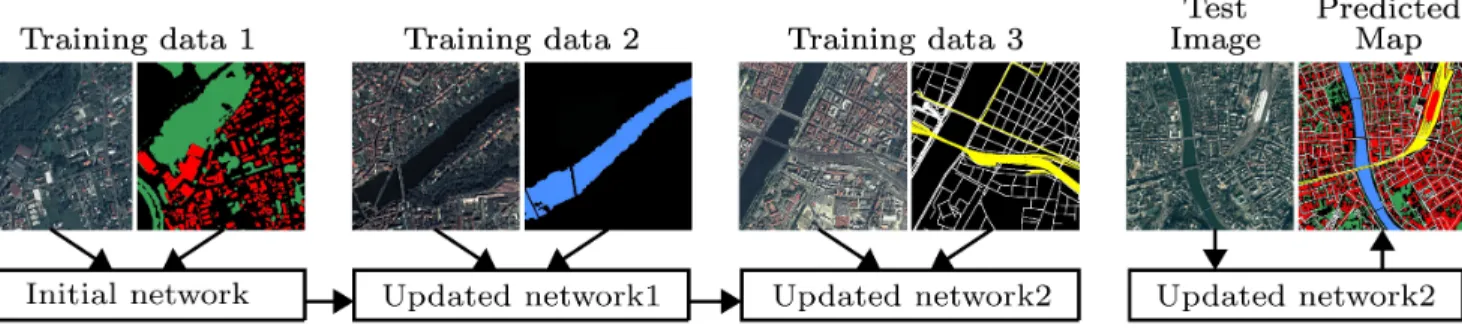
classes. Moreover, it may not always possible to store huge amount of data. Because of these reasons, it is of paramount importance to devise a classification system that can learn new classes continually while retaining performance for the old classes without accessing the entire previous data. The continual learning problem is illustrated in Fig. 1. To the best of our knowledge, in remote sensing community, this problem has not been explored yet.
The main drawback of the common CNNs for the con-tinual learning problem is that their performance for the old classes significantly drops when new classes are added to the trained model on the data, having no ground-truth for the pre-vious classes. The aforementioned abrupt performance loss is referred as catastrophic forgetting in the literature [2]. To overcome this problem, there have been some attempts, which change the network structure. An example methodology that is in this category is described in [3], where the network is expanded as new classes are added. The obvious limitation of this approach is that the network grows every time new classes are taught. Since deep neural networks contain mil-lions of parameters, different configurations of the parame-ters may produce the same results. Inspired from this idea, several works, which try to determine the important neurons and prevent them from changing drastically, have been pro-posed [4, 5]. The methodology propro-posed in [6] uses a small fraction of the previous training data to prevent forgetting the already learned information. The knowledge distillation from one network to another one [7] gave inspiration to several works. In [8, 9], the previous knowledge is distilled from the formerly trained network to the current one on the new data. Even though several methodologies have been proposed to overcome catastrophic forgetting, none of those works in-vestigates continual learning for dense labeling problem.
In this paper, we propose a method, which enables to learn dense labeling capabilities for the new classes without forget-ting the old classes even if the whole previous training data are not available.
2. METHODOLOGY
Our network structure is U-net, comprising an encoder that is architecturally the same as encoder of VGG-16 [10] and a symmetric decoder. Each convolution and deconvolution operation is followed by a rectified liner unit (ReLU). Since
Fig. 1. Continual learning problem. Every time new training data are retrieved, only a small potion of the previous ones are stored. The classes are building (red), tree (green), water (blue), road (white), and railway (yellow).
batch normalization uses the memory inefficiently, we prefer not to use it. The output of our network consists of binary predicted maps for all the classes.
Let us assume that the current training data are denoted by Dcurr. The sets of previously learned classes and the
classes in Dcurr are indicated by Lprev and Lcurr, where
Lprev ∩ Lcurr = ∅. During adaptation, we teach Lcurr
and Lprev to the network on Dcurr. Since the annotations
for Lprevare not available in Dcurr, we transfer the
knowl-edge from the memory network to the updated network. We denote by ycurr, the binary target vectors of the pixels in
a training batch from Dcurr for all the classes. We denote
the binary predicted probabilities for Lcurr and Lprev from
the updated network by ˆyup curr and ˆyup prev, respectively.
The predictions for Lprev from the memory network are
indicated by ˆymem. To learn Lcurr, we minimize the
clas-sification loss LclasssigmCE(ˆy
up curr,ycurr), which is the sigmoid
cross entropy loss between ˆyup curr and ycurr. In order to
distill the knowledge for Lprev from the memory network
to the updated network, we minimize the distillation loss Ldistil
sigmCE(ˆymem,ˆyup prev)that is the sigmoid cross entropy loss
between ˆymem and ˆyup prev. The loss that is minimized
during adaptation is defined as: Ladapt= LclasssigmCE(ˆyup curr,ycurr)+L
distil
sigmCE(ˆymem,ˆyup prev).
(1) For remembering, we store a little fraction of the previous training data. Because in satellite images number of samples for the classes are usually imbalanced, randomly selecting the training patches that would be stored might result in having no samples for the less frequent classes. Hence, we handle the class imbalance problem. Let us assume that D(j)previs the
jthprevious training data, and L(j)
prev denotes the classes in
D(j)prev. We compute a weight wcfor each class c ∈ L (j) previn D(j)prevas: wc = median(fc|c ∈ L (j) prev) fc , (2) where fc is frequency of the pixels, belonging to class c.
We then compute an importance value I(l)for the lthtraining
Small portion of
previous data 1 Currentdata Small portion ofprevious data 2 Currentdata
Fig. 2. Example optimization sequence. The sequence is: Lremon data 1, Ladapton the current data, Lrem on data 2,
and Ladapton the current data again.
patch in D(j)prevas:
I(l) = X
c∈L(j)prev
wcfc(l), (3)
where fc(l) denotes the number of pixels that are labeled as
class c in the patch. We store a certain number of patches, having the highest I values. In order to prevent storing only the patches that are located in very close geographic locations, we also store certain number of randomly selected patches. The number of patches that are selected randomly and using I values have to be determined. Let us assume that y(j)prev is
the target vector, and ˆy(j)up prevdenotes the predictions of the
pixels for L(j)previn the training batch from the stored, small
portion of Dprev(j) . The remembering loss Lremis defined as:
Lrem= LsigmCE(y(j)prev, ˆy (j)
up prev), (4)
where LsigmCE(y (j)
prev, ˆy(j)up prev) is the sigmoid cross entropy
loss between y(j)prevand ˆy (j)
up prev. The end user needs to
de-termine how frequently and on which previous training data, the samples would be fed to the network to optimize Lrem.
An example optimization sequence is depicted in Fig. 2. 3. METHODS USED FOR COMPARISON We compare our methodology with the following approaches:
Multiple learning: In this approach, we train a new net-work from scratch every time new training data are retrieved. Because of the growing number of classifiers, this learning approach is inefficient in terms of storage. Besides, since the
test images have to be segmented by each trained model to generate label maps for all the classes, the running time in the test stage might be very long.
Fixed representation : Whenever new training data are obtained, we increase the number of filters in the last con-volutional layer that is responsible for generating a binary predicted map for each class. In the training stage, we opti-mize only the filters for the new classes, and freeze the rest of the network. As we do not update the filters for the previous classes, the exact performance for them is retained. However, the network is not able to learn the new classes well, as the extracted features are not representative.
Fine-tuning: This approach is similar to fixed represen-tation. The difference is that we freeze only the filters for the previous classes in the last convolutional layer, and opti-mize the rest of the network. This methodology suffers from catastrophic forgetting.
Continual learning w/o rem.: This is our approach with-out optimizing Lrem. Since the whole network is adapted to
the last training data, the information learned from the previ-ous data might be forgotten.
4. EXPERIMENTS
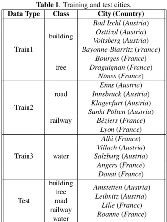
In our experiments, we use the Luxcarta dataset, which con-tains satellite images collected from 11 cities in France and 11 cities in Austria. The spatial resolution is 1 m. The full an-notations for building, tree, road, railway, and water classes are available. We use 9 cities from each country as the ing data, and the rest of the cities as test. We split the train-ing cities into three groups, as reported in Table 1. We as-sume that the cities in each group have annotations for only the classes that are indicated in the table. When dividing the training cities into groups, we make sure that cities in each group have acceptable number of samples for the indicated classes. We suppose that the training data are streamed in this order: Train1, Train2, and Train3. For our approach, we store 30% of the previous training patches, in which 15% are selected randomly and the other 15% are chosen using the I values. For the approaches described in Sec. 3, we do not use the previous training data.
In the pre-processing stage, we split all the training im-ages into 384×384 patches, having 32×32 pixels of overlap between the neighboring patches. We divide the test images into 2240×2240 patches with an overlap of 64×64 pixels. Af-ter classifying each test patch, we merge them back to get the final predicted maps. For the normalization, we subtract 127 from the pixels of each spectral band.
We train 3 models for multiple learning (one from each group) for 500 epochs, where each epoch consists of 100 iter-ations. For the rest of the approaches, whenever new training data are retrieved, we update the previous model by training for the same number of epochs and iterations as for multiple learning. For continual learning, when we add road and rail-wayclasses on Train2 to the model trained on Train1, we
op-Table 1. Training and test cities. Data Type Class City (Country)
Train1
building
Bad Ischl(Austria) Osttirol(Austria) Voitsberg(Austria) Bayonne-Biarritz(France) tree Bourges(France) Draguignan(France) Nˆımes(France) Train2 road Enns(Austria) Innsbruck(Austria) Klagenfurt(Austria) railway
Sankt P¨olten(Austria) B´eziers(France) Lyon(France) Train3 water Albi(France) Villach(Austria) Salzburg(Austria) Angers(France) Douai(France) Test building Amstetten(Austria) tree Leibnitz(Austria) road Lille(France) railway Roanne(France) water
timize Ladaptfor 4 iterations and Lremfor 1 iteration. To add
waterclass on Train3, the optimization sequence is: Ladapt
for 2 iterations, Lremon Train1 for 1 iteration, Ladaptfor 2
iterations, and Lremon Train2 for 1 iteration. We use Adam
optimizerto optimize parameters of the networks. The learn-ing rate is 0.0001 and exponential decay rate for the first and the second moment estimates are 0.9 and 0.999. Each train-ing batch consists of 12 patches. When sampltrain-ing a patch, we first randomly select a country. We then choose a random city from the selected country. We finally randomly pick a training patch from the chosen city. In the training stage, we augment the training patches with 0/90/180/270 degrees of random ro-tation, random horizontal and vertical flips, random contrast change, and gamma correction.
F1-scores [11] of each method for all the classes are re-ported in Table 2. Close-ups from the generated maps for multiple learning, continual learning w/o Lrem, and
contin-ual learningare shown in Fig. 3. Although the output of our network architecture is a binary classification map for each class, to visualize the outputs more compactly, we provide multi-class maps in the figure by assigning each pixel to the class, having the highest probability. As expected, fixed repre-sentationcan not learn new classes very well, and fine-tuning catastrophically forgets the previously learned classes. For our approach, if we do not remind information from the pre-vious data, performance for the already learned classes might
Table 2. F1 scores on the Luxcarta dataset.
Method Epoch Building Tree Road Railway Water Overall multiple learning 500 71.25 68.88 59.28 55.65 79.83 66.98 fixed representation 1000 71.25 68.88 2.71 0.00 — 1500 71.25 68.88 2.71 0.00 0.11 28.59 fine-tuning 1000 28.91 0.17 59.30 60.06 — 1500 27.90 7.71 0.14 0.01 90.20 25.19 continual learning 1000 74.19 66.32 56.57 50.87 — w/oLrem 1500 74.91 66.87 58.14 51.70 82.32 66.79 continual learning 1000 75.98 72.38 57.29 50.18 — 1500 76.78 72.06 59.58 53.07 78.94 68.09 Training Set 1 Training Set 2 Training Set 3
Image GT mult. lear. cont. lear. cont. lear. w/oLrem
Amstetten
Leibnitz
Lille
Roanne
Fig. 3. Close-ups from the test cities. Classes: background (black), building (red), road (white), railway (yellow), high vegetation (green), and water (blue).
decrease over time. For instance, for tree class, performance of continual learning w/o Lremis lower than multiple
learn-ingand continual learning. For multiple learning, learning for each class is limited to the images from only one group, which may cause showing a lower performance. E.g., build-ingclass is learned from only the images in Train1. Therefore, performance for this class is lower than our approach. As the proposed continual learning approach enables to both learn from the new data and remember from the previous data, it exhibits the best performance for most of the classes.
5. CONCLUDING REMARKS
We proposed a novel continual learning approach, enabling to learn segmenting new classes without deteriorating perfor-mance for the old classes, although a small portion of the pre-vious training data are accessible. As the future work, we plan to incorporate domain adaptation techniques into the pro-posed continual learning approach so that new classes could be learned successfully, even when there is a large domain
shift between the previous and the current training images. 6. REFERENCES
[1] B. Huang, K. Lu, N. Audebert, A. Khalel, Y. Tarabalka, J. Malof, A. Boulch, B. Le Saux, L. Collins, K. Brad-bury, et al., “Large-scale semantic classification: out-come of the first year of inria aerial image labeling benchmark,” in IEEE IGARSS, 2018.
[2] I. J. Goodfellow, M. Mirza, D. Xiao, A. Courville, and Y. Bengio, “An empirical investigation of catastrophic forgetting in gradient-based neural networks,” arXiv, 2013.
[3] S. S. Sarwar, A. Ankit, and K. Roy, “Incremental learn-ing in deep convolutional neural networks uslearn-ing partial network sharing,” arXiv, 2017.
[4] J. Kirkpatrick, R. Pascanu, N. Rabinowitz, H. Veness, G. Desjardins, A. A. Rusu, K. Milan, J. Quan, T. Ra-malho, A. Grabska-Barwinska, et al., “Overcoming catastrophic forgetting in neural networks,” Proceed-ings of the national academy of sciences, p. 201611835, 2017.
[5] R. Aljundi, F. Babiloni, M. Elhoseiny, M. Rohrbach, and T. Tuytelaars, “Memory aware synapses: Learning what (not) to forget,” arXiv, 2018.
[6] S.-A. Rebuffi, A. Kolesnikov, G. Sperl, and C. H. Lam-pert, “iCaRL: Incremental classifier and representation learning,” in CVPR, 2017.
[7] G. Hinton, O. Vinyals, and J. Dean, “Distilling the knowledge in a neural network,” arXiv, 2015.
[8] Z. Li and D. Hoiem, “Learning without forgetting,” IEEE TPAMI, 2017.
[9] K. Shmelkov, C. Schmid, and K. Alahari, “Incremental learning of object detectors without catastrophic forget-ting,” in ICCV, 2017, pp. 3420–3429.
[10] K. Simonyan and A. Zisserman, “Very deep convo-lutional networks for large-scale image recognition,” arXiv, 2014.
[11] N. Audebert, B. Le Saux, and S. Lef`evre, “Seman-tic segmentation of earth observation data using mul-timodal and multi-scale deep networks,” in ACCV. Springer, 2016, pp. 180–196.