HAL Id: halshs-03244647
https://halshs.archives-ouvertes.fr/halshs-03244647
Preprint submitted on 1 Jun 2021
HAL is a multi-disciplinary open access
archive for the deposit and dissemination of sci-entific research documents, whether they are pub-lished or not. The documents may come from teaching and research institutions in France or abroad, or from public or private research centers.
L’archive ouverte pluridisciplinaire HAL, est destinée au dépôt et à la diffusion de documents scientifiques de niveau recherche, publiés ou non, émanant des établissements d’enseignement et de recherche français ou étrangers, des laboratoires publics ou privés.
’Bad’ Oil, ’Worse’ Oil and Carbon Misallocation
Renaud Coulomb, Fanny Henriet, Léo Reitzmann
To cite this version:
Renaud Coulomb, Fanny Henriet, Léo Reitzmann. ’Bad’ Oil, ’Worse’ Oil and Carbon Misallocation. 2021. �halshs-03244647�
WORKING PAPER N° 2021 – 38
’Bad’ Oil, ’Worse’ Oil and Carbon Misallocation
Renaud Coulomb Fanny Henriet Léo Reitzmann
JEL Codes: Q35, Q54, Q58, L71.
Keywords: climate change, oil, carbon mitigation, misallocation, stranded assets.
’Bad’ Oil, ’Worse’ Oil and Carbon Misallocation
∗
Renaud Coulomb
a, Fanny Henriet
b, L´eo Reitzmann
cMay 2021
Abstract
Not all barrels of oil are created equal: their extraction varies in both private cost and carbon intensity. Using a rich micro-dataset on World oil fields and estimates of their carbon intensities and private extraction costs, this paper quantifies the additional emissions and costs from having extracted the ’wrong’ deposits. We do so by com-paring historic deposit-level supplies to counterfactuals that factor in pollution costs, while keeping annual global consumption unchanged. Between 1992 and 2018, carbon misallocation amounted to at least 10.02 GtCO2 with an environmental cost evaluated at US$ 2 trillion (US$ 2018). This translates into a significant supply-side ecological debt for major producers of dirty oil. Looking towards the future, we estimate the gains from making deposit-level extraction socially-optimal, and document the very unequal distribution of the subsequent stranded oil reserves across countries.
Keywords: Climate change, oil, carbon mitigation, misallocation, stranded assets. JEL Codes: Q35, Q54, Q58, L71.
∗We thank seminar participants at the Paris School of Economics, the Toulouse School of Economics,
the University of Amsterdam, the Graduate Institute Geneva, the Banque de France, and participants at the 11th FAERE Thematic Workshop “Energy transition” in Paris. We are grateful to Jeff Borland, Julien Daubanes, Antoine Dechezlepretre, John Freebairn, Geoffrey Heal, Leslie Martin, Rick van der Ploeg, and Yanos Zylberberg for their helpful comments, and L´eo Jean for outstanding research assistance. We also thank Mohammad S. Masnadi for sharing part of the data used in our robustness checks. Financial support from the Agence Nationale de la Recherche (ANR-16-CE03-0011 and EUR ANR-17-EURE-0001) is gratefully acknowledged.
aUniversity of Melbourne, 111 Barry Street, VIC 3010, Australia. E-mail:
re-naud.coulomb@unimelb.edu.au.
bParis School of Economics-CNRS: 48 Bd Jourdan, 75014 Paris, France. E-mail:
fanny.henriet@psemail.eu.
1
Introduction
Oil deposits vary in their private and social marginal extraction costs. These two costs differ markedly as oil extraction generates substantial Greenhouse gas (GhG) emissions that are not internalized by oil producers. These emissions vary across deposits, and depend on oil and reservoir characteristics and the associated extractive technologies (Masnadi et al.,
2018). For instance, producing a barrel of crude from bitumen in Canada emits twice as much Greenhouse gas as a barrel of light crude from Saudi Arabia. As keeping the rise in global temperature below 2°C requires leaving large oil reserves forever untapped (Meinshausen et al.,2009), choosing the right deposits to exploit can be a key lever for emission abatement in a sector that is otherwise difficult to decarbonize (Creutzig et al.,2015). However, despite the global recognition of the climate-change risk, since at least the 1992 Earth Summit, production-related GhG emissions from oil have mostly been ignored (World Bank, 2020). Poor or absent regulations are a major source of carbon misallocation in this industry, with dirty oil (e.g., heavy oils) being extracted instead of lower carbon-intensity oil.
This paper is the first to quantify the environmental cost of misallocation in oil supply. We leverage a rich micro-dataset of World oil fields and estimates of their carbon intensities and private extraction costs to measure the additional emissions and costs of historic oil supply since the 1992 Earth Summit as compared to the socially-efficient allocation. We then assess the social gains of optimal future supply, compared to a competitive extraction that matches the same aggregate supply path. Overall, we show that supply recomposition, through the choice of the cumulative amount to be extracted from each deposit and the sequencing of deposits use, can produce large emission reductions at zero or low cost, while leaving the demand-side unchanged.
Our estimation of past carbon misallocation relies on the difference in cumulative pol-lution between the historic oil-supply curve and the socially-optimal counterfactual that minimizes environmental and private extraction costs, while leaving annual global aggregate extraction unchanged. As any barrel used before 2018 is no longer available in the future, our measure of past misallocation accounts for the opportunity costs attached to the ex-traction of barrels in the past. More precisely, our counterfactual takes oil to be optimally extracted from 1992 up to 2050, the date at which carbon neutrality is reached (IPCC,2018;
European Council, 2019). This counterfactual is compared to the extraction path from the historic 1992-2018 supply and a future supply (with the same annual global production up to 2050) that we take to be either competitive and ignoring pollution heterogeneity, or optimal.1
1We also consider alternative dates for carbon neutrality (2066 and 2080), with similar results. As
our supply recomposition does not come with a change in aggregate supply, the ’optimal counterfactual’ is actually the optimal structure of the aggregate supply, and thus represents a second-best.
Our central findings indicate that inefficient emissions from oil misallocation over the 1992-2018 period amount at least to 10.02 gigatons of CO2 (GtCO2). These emissions are
substantial, representing two years of life-cycle emissions of the global transportation sector, and their cost is estimated at 2 trillion US$.2 We also find that the optimal allocation of
extraction across deposits results not only in less carbon-intensive extraction but also lower private extraction costs, as our optimal counterfactual solves both carbon mispricing and other market imperfections. Though the historic deposit-level supplies reveal that deposits’ carbon heterogeneity was ignored and extraction was not competitive, we document that inefficient emissions can be attributed to carbon mispricing, rather than imperfect competi-tion. Solving only private cost misallocation in oil supply, that is expensive oil was extracted in lieu of cheaper oil, while ignoring pollution reduces cumulative emissions by 1.87 GtCO2
only. Thus, carbon misallocation is distinct from private cost misallocation.
In a next step, we use our deposit-level data to map countries’ supply-side ’ecological debts’, i.e., their over-extraction from the comparison of their aggregate historical supply to their optimal supply. This allows us to determine the winners and losers from carbon misallocation. We in particular show that Annex B countries, which committed to mitigation targets in the 1997 Kyoto Protocol, over-extracted oil by 66% in the 1992-2018 period, whereas the Rest of the World under-extracted by 30%.
We then evaluate the gains from the optimal extraction of resources in the future, as compared to a perfectly-competitive future supply with identical annual demands in which pollution heterogeneity is ignored. Extracting oil optimally starting in 2019 yields future emission savings of 7.64 GtCO2. We then estimate the stranded reserves of oil-producing
countries, i.e., the share of their 2019 oil reserves that should optimally remain underground. These vary widely across countries, from a figure of 15.3% in Kuwait to 97.4% in Canada.
Finally, we consider alternative dates to start the recomposition of past supply, as the 1992 Earth Summit was not the only missed window of opportunity. We show that starting to extract optimally one year earlier always yields large additional environmental benefits, even for periods that are as far in the past as the 1970s. We also show that the post-2010 rise in US Shale Oil production and Canada’s Oil Sands production, which are expensive to extract, and the ‘Oil Counter-Shock’ (1980-1986) are behind substantial misallocation.
Our findings inform the debate on climate-change mitigation costs, and produce three key policy recommendations. First, as the variation in crude-oil carbon intensity originates in the upstream and midstream sectors, any regulation of downstream emissions (combustion)
2These results are derived for a social cost of carbon (SCC) of US$ 200 per ton of CO
2 in 2018, in line
with Lemoine (2021) and the DICE2016R scenario of keeping the temperature rise below 2.5°C over the
next 100 years (Nordhaus,2017). The inefficient emissions in the past are of the same magnitude for a large
that treats all crudes similarly misses out on important mitigation opportunities.3 A second
policy recommendation concerns what can still be changed in the future. We document that, as the opportunity costs of using good resources are only small, delaying mitigation is costly. The post-2018 gains from optimal extraction would be almost the same were oil to have been extracted optimally since 1992. A third important message is that the misallocation attributable to poor carbon regulation has little in common with production inefficiencies arising from OPEC’s market power. The need for environmental regulations should not be confused with pro-competition policy and should receive the same attention from policymakers.
Optimal extraction entails a large reallocation of aggregate production between coun-tries, as compared to observed extraction pre-2019. This reallocation may be difficult to implement politically, due to country preferences for domestic productions, e.g. job-related, public-finance or energy-security concerns, or difficulties in setting up international com-pensation. Recomposing supply without changing countries’ observed annual production still yields large emission reductions of about 9.57 GtCO2 over the 1992-2018 period, which
is due to significant within-country heterogeneity in carbon intensities. Overall, limiting
country-level production changes still leaves large potential gains from (past or future)
sup-ply recomposition, which alleviates feasibility concerns. Which policy instruments should be used to attain the recommended deposit-level supplies? Carbon pricing on the supply-side is obviously an interesting instrument but may face obstacles such as lobbying activities of firms, non-cooperative countries that refuse to implement the tax domestically, or tax-incidence issues that arise from the finite nature of oil deposits (Heal and Schlenker, 2019). An alternative would be to prevent any country from consuming dirty oil, in a supply-side policy `a la Harstad(2012). Precluding extraction from dirty-oil deposits and then extracting other deposits in a competitive way without further pollution considerations so as to obtain the same emission reduction as under optimal supply, would raise private extraction costs by 1.6 trillion US$ compared to optimal extraction.
This paper is the first to empirically assess inefficiencies in global oil production, factoring in pollution. Environmental concerns are largely absent from the literature on
misalloca-3Upstream regulation is usually out of scope for most consumer countries, although attempts have been
made to reduce the life-cycle emissions of fuels. An example is the EU’s Fuel Quality Directive (FQD), the
purpose of which is to reduce automotive-fuels carbon footprints in 2020 by 6% compared to 2010 (Malins
et al.,2014a). Each fuel supplier has to achieve the 6% reduction target but all suppliers report annually the same EU-wide carbon intensity value for fossil petrol and diesel, whether their products originate from high-carbon sources or not. Mitigation assessments in the transport sector tend to ignore oil-supply recomposition (Replogle et al., 2013; Vimmerstedt et al., 2015) but focus on fuel switching, e.g., from oil to natural gas,
bio-methane or bio-fuels, (Sims et al., 2014), despite potentially large adjustment costs (due to fuel-specific
existing installations, for example) and industry lobbying efforts against the transition (Knaus,2019;Lipton,
tion, with the exception of some recent contributions: Sexton et al. (2018) and Lamp and Samano (2020) examine environmental misallocations in residential solar installations and
Correa et al. (2020) in the copper industry. Our methodology is close to Borenstein et al.
(2002) and Asker et al.(2019), who relate misallocation in production factors to the under-utilization of observed lower-cost production units in a given sector.4 Our paper builds upon
the analysis of production misallocation due to market power in the oil industry in Asker et al.(2019). In contrast to their work, we consider an additional source of social inefficiency: heterogeneity in the carbon externality associated with extraction and refining. The only source of inefficiency in observed production in their paper comes from resource-extraction sequencing that does not correspond toHerfindahl 1967’s “least-cost first” rule, i.e. extract-ing the cheapest resource first, as all deposits are eventually exhausted. By way of contrast, many deposits in a carbon-constrained world should be left untapped forever or be only partially exploited, and optimal deposit-selection depends on the trade-off between the eco-nomic and environmental costs.5 This trade-off is empirically significant. At the fine level of
disaggregation of our data, carbon intensities and private extraction costs are not strongly correlated, so the inefficiencies from omitted pollution costs do not mirror extraction-cost in-efficiencies. We compute the total cost of misallocation attributable to OPEC market power as the cost of moving from the optimal supply to the second best supply obtained under the constraint that each OPEC’s country keeps the same annual production as observed in the data. We show that this cost is of the same order of magnitude as the misallocation cost attributable to carbon mispricing, i.e. the cost of moving from the optimal supply to a competitive supply in which pollution is ignored.
Our findings contrast with recent theoretical literature (Benchekroun et al., 2020) that has used a two-resource model to show how cartels like OPEC can actually speed up pollution by enabling producers of expensive and dirtier resources to enter the market earlier than they would have under perfect competition. We show that this mechanism is indeed at work here, but accounts for only a small part of carbon misallocation: switching to the competitive supply brings about an emission reduction that is about one tenth of that of the optimal supply structure over the 1992-2050 period. There is significant pollution heterogeneity in the
4A large body of literature analyzes the impact of misallocation on economic objects such as TFP (see
e.g., Hsieh and Klenow 2009) or focuses on the possible sources of misallocation (e.g., Hopenhayn and
Rogerson,1993;Guner et al.,2008;Restuccia and Rogerson,2008); seeHopenhayn(2014) for a review.
5Furthermore, ’oil abundance’ and the presence of capacity constraints have considerable implications for
the order of extraction: resources extracted along the optimal path are not necessarily extracted “least-cost
first”. Theoretical work has analyzed the extraction of multiple polluting resources (Chakravorty et al.,2008;
Van der Ploeg and Withagen,2012;Michielsen,2014;Fischer and Salant,2017;Coulomb and Henriet,2018). However, the literature is almost silent on the properties of the optimal extraction of multiple exhaustible resources that differ in both their private extraction costs and pollution content.
oil available within (or outside) OPEC, and there are cheap but polluting resources within (or outside) OPEC. This explains why a cost-effective supply brings little environmental gain, so that OPEC market power contributes little to carbon misallocation.6
BothAsker et al. (2019) and Benchekroun et al.(2020) relate supply inefficiencies to the wrong sequencing of deposits only: as all deposits are exhausted, there is no selection as to which to use and which to leave. On the contrary, we highlight that, in a carbon-constrained world, the selection of the deposits to use is key for lower social-extraction costs. In our setting, while 88% of extraction-cost misallocation can be attributed to the wrong order of resource extraction, all of the environmental gains come from the selection of deposits.
Last, we contribute to the literature on stranded assets. The scientific literature has raised awareness of the issue of unburnable fuels (Meinshausen et al.,2009; McCollum et al.,2014) and their unequal distribution (McGlade and Ekins, 2015). Recent research (McGlade and Ekins, 2014; Brandt et al., 2018) has acknowledged that oil carbon-intensity heterogeneity should be accounted for to mitigate future emissions, but does not provide any measure of carbon misallocation. As such, McGlade and Ekins (2014) and Brandt et al. (2018) do not explore the trade-off between production costs and emission reductions. In contrast, we look at the social cost of extracting from the wrong deposits in the past and the future, and quantify carbon misallocation.
The remainder of this paper is organized as follows. Section 2 describes the oil-deposit microdata and the estimation of deposit-level carbon intensities. Section 3 sketches the method used to quantify carbon misallocation in oil supply, and how we disentangle this from inefficiencies in private extraction costs. Section 4 then presents our results and their sensitivity to changes in the main assumptions. Last, Section 5concludes and elaborates on ways to implement field-level supply changes.
2
Oil data, extraction costs and carbon intensities
Quantifying the carbon misallocation from the use of ‘wrong’ deposits (from a climate-wise perspective) first requires us to estimate field-level carbon intensities and private production costs. In particular, we need to have data on the carbon intensities and costs of those sections of the oil-supply chain in which these vary significantly across barrels. Our analysis
6Market power has been considered rather positively through the lenses of resource conservation
(Hotelling, 1931; Solow, 1974), and thus pollution mitigation. We do not analyze the impact of market power on aggregate supply, as we want to keep the global oil consumption stream unchanged in order to quantify supply-side misallocation: the aggregate supply is thus considered exogenous. Furthermore,
analyz-ing the nature of OPEC market power (Hansen and Lindholt,2008) and its interaction with carbon policies
thus focuses on upstream (oil extraction) and midstream (refining) carbon intensities7 and
extraction costs.8
This section briefly presents the oilfield data (see Appendix A for a more-detailed de-scription). We then explain how we calculate field-level private extraction costs. Finally, we describe how we estimate carbon intensities.
2.1
Oil-deposit data
The Rystad Upstream dataset. Our empirical analysis is based on one of the most-comprehensive datasets of oil fields, the Rystad UCube Database (Rystad, afterwards). This covers most of World oil production, with 12,463 active deposits between 1970 and 2018. It includes precise field-level data on oil production, exploitable reserves, discoveries, capital and operational expenditures from exploration to field decommission, current gover-nance (e.g., ownership and operators), field-development dates (discovery, license, start-up, and production end), and oil characteristics (e.g., oil type, density and sulfur content) and reservoir information (e.g., water depth, basin and location).
The Rystad dataset does not contain information on fields’ upstream carbon intensities. However, it does record the key variables that influence emissions from extraction or refining, such as oil type (e.g., bitumen or light), API gravity, gas-to-oil ratio, sulfur content, use of steam injection, and the location of the field offshore or onshore.
Additional data. Two extraction techniques that affect emissions from extraction— methane flaring and steam injection— are not recorded precisely in Rystad. Flaring consists in the burning on-site of the methane that comes with oil. This mitigates the risk of explo-sion from methane accumulation near an installation. As only a minority of countries and companies collect and publish data on flared gas, this information is missing for nearly 95% of the fields in Rystad. We complement these data using the geocoded flaring volumes cal-culated by the Visible Infrared Imaging Radiometer Suite (VIIRS) algorithm from National Oceanic and Atmospheric Administration (NOAA) satellite observations. Steam injection is a thermal Oil Enhanced Recovery (EOR) technique employed in some fields—mostly those producing heavy oil— to facilitate extraction. Rystad data identify the use of steam injection
7See AppendixB.3for a discussion of downstream emissions. In a nutshell, downstream emissions include
mostly combustion-related emissions and transport to the end consumer. Combustion-related emissions are
large (an average of 75.82 gCO2eq/MJ, weighted by 2018 production) but do not vary much by crude origin
for a given end-use. Transport emissions to consumers will be affected by the recomposition of supply. However, these emissions are small and do not vary much. We therefore restrict our main analysis to upstream and midstream sectors, where carbon-intensity heterogeneity is found.
8Midstream and downstream costs vary by oil, but are small relative to the standard deviation of crude
only for bitumen fields. We add steam-injection data from the International Energy Agency (IEA, 2018b).
2.2
Deposit extraction costs
The annual field expenditures reported in Rystad database are “well” and “facility” capital expenditures, and “selling, general and administrative”, “transportation” and “production” operational expenditures.
For each deposit, we assume that the total present cost of extracting any stream of production (xdt), from exploration to shutdown [t1; t2], can be written as Ptt21cdxdte
−rt, so
that cd can be estimated as the levelized cost of extraction (LCOE) of the field. Denoting
by xdt the annual deposit production, cdt total opex and capex expenditures of deposit d
in year t as reported in Rystad, and r the annual discount rate (set at 3%), the levelized cost of extracting a barrel from deposit d over its life from exploration to shutdown [t1; t2] is
cd= (Ptt21cdte
−rt)/(Pt2
t1xdte
−rt). This represents the field break-even price or the equivalent
constant cost of a barrel for a field over its lifetime. In this approach, extraction costs are exogenous to the policies implemented, as in Asker et al. (2019). This echoes that extraction methods, field installations and energy needs are largely determined by exogenous factors such as the physical properties of the hydrocarbons (e.g., viscosity and density) and the reservoir geophysical characteristics (e.g., rock porosity and permeability, and reservoir complexity and depth). For instance, oil located in ultra-deep or complex reservoirs is more expensive to extract (IEA, 2008).
We consider other definitions of field-level private extraction costs in our robustness checks. We first use average cost instead of LCOE. Second, we deduct expenditures and production that occurred before the starting date of optimization from the LCOE calculation, in order to account for potential sunk start-up costs. Third, we allow private extraction cost to vary over time, assuming the existence of two exogenous Martingale processes governing input costs (one common to all onshore fields and the other common to all offshore fields), to account for potential annual shocks on input prices, in line with Asker et al. (2019).
Appendix C.3 describes the data, our main approach to calculate field-level private ex-traction costs, and the alternative cost measures.
2.3
The carbon intensity of deposits
Upstream carbon intensity. Before oil extraction starts, GhG emissions are generated from field exploration and the setting up of injecting and extracting wells.9 After production
begins, activities such as well maintenance, oil extraction and surface processing, as well as transport to the refinery inlet, emit GhG emissions.
Field-level carbon intensities are assumed to be exogenous to carbon policies and time-invariant in our main approach: this reflects the role of exogenous factors, such as oil viscosity and density in emissions from extraction and refining. Emissions are also linked to extraction techniques, which are largely tied to oil type. For example, lifting heavy oils requires a more intensive use of Enhanced Oil Recovery (EOR) techniques, such as thermal EOR or Gas-EOR. Another example is flaring: when crude oil is extracted from oil wells, the natural gas associated with the oil is brought to the surface at the same time, and vast amounts of this gas is commonly flared as waste. Flaring is typically associated with high carbon intensity, and is largely determined by exogenous factors such as the reservoir’s gas-to-oil ratio and the distance to a significant consumer market for gas. Less flaring could, however, in theory be implemented by operators. We abstract from this possibility in our main specification for two reasons. First, abatement-cost estimates vary significantly across studies, and no field-level estimates are available for global oil production (Malins et al.,2014b). Second, flaring regulation seems to be ineffective globally (Farina, 2011; Calel and Mahdavi, 2020), and even counterproductive if as little as 7% of the non-flared methane is instead vented directly into the atmosphere, due to the much greater warming potential of methane as compared to carbon dioxide. As Calel and Mahdavi (2020) note, whereas flares are visible to remote-sensing instruments, vented gas is on the other hand invisible: this casts doubt on whether flaring reductions genuinely correspond to lower GhG emissions. Due to data limitations on the field-level costs of abating flaring emissions, and the difficulty in relating less flaring to true GhG-emission reductions, our main specification will assume fixed field flaring-to-oil ratios (FORs). Overall, our approach (fixed technologies) is conservative, as allowing for endogenous technology changes would bring larger environmental gains. In a robustness check, we update upstream carbon intensities with a 10% lower field-level flaring-to-oil ratio (FOR) at no cost.
We use the Oil Production Greenhouse Gas Emissions Estimator (OPGEE) of the Oil-Climate Index (OCI, Carnegie Endowment for International Peace) to estimate upstream emissions. We proceed as follows: we first run the OPGEE using data on 958 deposits, formatted to be used as model inputs and publicly available from Masnadi et al. (2018).
9We will use the terms carbon emissions, pollution and CO
2to refer to GhG emissions. All CO2quantities
These represent 54% of 2015 World production. We then match these deposits to those in the Rystad dataset, and select the estimation model that best explains OPGEE car-bon intensities using the variables in the Rystad dataset and supplementary sources (IEA and NOAA-VIIRS). The explanatory variables are selected based on the scientific literature (Brandt et al.,2015; Gordon et al.,2015;Masnadi et al.,2018). We find that field upstream carbon intensity varies by oil type (e.g., regular or heavy), the gas-to-oil and flaring-to-oil ratios, and the use of steam injection. Offshore location and operator size also play a role, but to a lesser extent. The chosen reduced-form model with these explanatory variables yields an Adjusted R-squared of 0.95 (Appendix Table B1). Finally, we predict the carbon intensities of the remaining fields in the Rystad dataset using this model. These predicted values are robust to changes in the sample of fields used to estimate the model.10 Our
esti-mates are consistent with those in the scientific literature (Appendix Figure B3). Appendix
B.1 describes OPGEE, the matching procedure and results, the estimation model and the robustness checks in more detail.
Midstream carbon intensity. After reaching a refinery, crude oil from different fields is combined and refined into petroleum products, such as gasoline and other fuels. Refining processes emit mostly CO2, CH4 and N2O that are the main GhG sources of this sector.
We employ the OCI Petroleum Refinery Life-Cycle Inventory Model (PRELIM)11 to assess
midstream carbon intensities (see Appendix B.2). This engineering-based model requires very detailed information on the physical and chemical properties of oils (“crude assays”). As detailed oil properties are only partially available in Rystad, we proceed as follows. We first run PRELIM with the 149 assays of major oil crudes (from companies, specialized websites and past research) that are publicly available with PRELIM. We associate these crudes to their extraction site using operator and crude names, and location information in Rystad data. We then estimate PRELIM carbon intensities using the Rystad variables related to oil characteristics and known to impact refining carbon intensity: the API gravity index and the sulfur content. These determine the main refining configuration (deep/medium conversion or hydroskimming), that is the level of processing intensity.12 Our approach
10AppendixBincludes a series of robustness checks regarding CI estimation. We first investigate its
po-tential sensitivity to some observations. The bottom panel of Appendix Figure B1presents the correlation
coefficients of OPGEE carbon intensities and the predicted values obtained when estimating (9) after having
removed the OPGEE fields one-by-one, while Appendix Figure B2 depicts how the coefficients on the
ex-planatory variables vary. We then consider model behavior when excluding a set of “influential” observations
instead of each single observation (Appendix Table B2.) The definition of influential observations is based
on Cook’s distance. Overall, our model is robust to changes in the sample of deposits used to estimate (9).
11PRELIM and OPGEE use the same units of energy, and are designed so that their carbon intensities
can be summed to track emissions from oil exploration through refining.
12A dummy for the largest private oil companies (the “Majors”) is also added to capture unobservable
assumes that refineries are fixed,13 so that heterogeneity in pollution due to installations or
country particularities (from local air pollutant regulations, for example) can be ignored. We here focus on those midstream emissions that are tied to the nature of the extracted oil, i.e. that could be affected by a change in deposit extraction. Our parsimonious model explains more than half of the total variance in midstream carbon intensity. Last, we predict midstream CI for the rest of the crudes/fields in the Rystad dataset.
2.4
Descriptive evidence
This section provides descriptive evidence that: (i) the carbon intensity of oil extraction (and that of crude refining to a lesser extent) differs significantly across deposits; (ii) car-bon intensities and private extraction costs are not strongly correlated; and (iii) proven oil reserves exceed climate-wise future demand.
Carbon intensity varies across oil deposits. From our estimation, the average upstream carbon intensity of oil in 2018 was 10.15 gCO2eq/MJ, while average midstream
carbon intensity was 5.15 gCO2eq/MJ. Both upstream and midstream emissions vary across
deposits. The distribution of upstream carbon intensities has considerable variance: 25% of the upstream CI distribution is under 6.65 gCO2eq/MJ, 50% under 8.55, and 75% under
10.84. There is less variance in midstream carbon intensity: 25% of the midstream CI distribution is under 4.24 gCO2eq/MJ, 50% under 4.87, and 75% under 5.19.
The combined upstream and midstream carbon intensities of oils extracted since 1992 vary by oil type (Figure 1(a)). Unconventional oils, such as heavy and extra-heavy oils, are about twice as polluting as conventional oils, such as light oils. Flaring and steam injection also play a role, and partly explain the large variation in carbon intensity within oil categories. As countries have different kinds of oils, the average carbon intensity of an oil barrel varies by country of extraction (Figure 1(b)): oil extracted in Indonesia, Algeria, Venezuela and Canada emits about twice as many emissions than the average barrel pumped in Saudi Arabia or Kuwait. There exists significant within-country heterogeneity: for instance, Canada is host to very different types of oils (oil sands, shale oil, conventional oil), whereas some other countries, such as Saudi Arabia or Kuwait, have more homogeneous oil located in only a few fields. OPEC members (the grey bars in the figure) are not a homogeneous group in terms
physical properties of their oils. This dummy has little influence on emissions.
13Assuming that refining technologies could change, or new refineries could be set up with the
best-in-class climate-wise process, would add another lever of carbon mitigation and bring overall larger emission
reductions (Jing et al., 2020). Our approach also assumes that refineries that treat heavy and extra heavy
oil can be reconfigured at low cost to refine lighter oil. This assumption is consistent with heavy oil refining
requiring complex configurations of refining units that include those used to refine lighter oils (see e.g., U.S.
of oil carbon intensity. As is apparent in Figures 1(a)-1(b), since 1992, polluting oil types have been extracted, refined and combusted instead of cleaner — and sometimes cheaper — alternatives.
Little correlation between carbon intensities and private extraction costs. Private extraction costs also differ across deposits. These vary with oil type (Appendix Figure C1, top panel), which translates into some countries, e.g. Kuwait, having average extraction costs around three to four times cheaper than those in countries with the most expensive oil, e.g. Canada and Brazil (Appendix Figure C1, bottom panel). These figures are consistent with the rankings based on country of extraction or/and oil types in IEA
(2008) and Wood Mackenzie(2019).
At the fine level of disaggregation of our data, there is only little correlation between car-bon intensity and private extraction costs (Appendix FigureF1).14 Introducing
production-based (the dashed best linear fit line) or reserve-production-based (the unbroken best linear fit line) weights does not change this conclusion: the low correlation applies to both barrels that have been extracted and barrels that are available for extraction. We then conjecture that cost-effective carbon mitigation in the oil industry implies a very different extraction path to that under a pro-competition policy that ignores pollution.
Too much oil. The scientific literature has highlighted that oil assets are too abundant, given the estimated carbon budgets, to keep the average-temperature increase under 1.5 or 2°C throughout the century (Meinshausen et al., 2009; McCollum et al., 2014; McGlade and Ekins, 2014). The back-of-the-envelope calculation in Covert et al. (2016) suggests that burning all fossil fuels in proven reserves would lead to a temperature rise of between 5.6 and 8.3°C. Using our carbon intensity estimates, extracting, refining and burning all proven reserves of oil (as recorded in Rystad) would generate about 692.5 GtCO2, which is
between 1.6 and over 3 times the average total remaining carbon budget (that encompasses emissions from oil, gas and coal, and land transformation) required to keep the temperature increase below 1.5°C (IPCC,2014,2018;Rogelj et al.,2019).15 Figure2(a)depicts the carbon
intensity of remaining recoverable reserves in 1992—the year of the Rio Summit—together with the post-1992 demand to fulfill; these reserves vary significantly in carbon intensity, and more than half should be left untapped. These reserves also differ by private extraction cost (Figure2(b)), and carbon intensity varies significantly within each bin of costs.
14The correlation coefficients between carbon intensity and private extraction costs are 0.07 and 0.05 when
deposits are weighted by their 1992 reserves and total productions over the period 1992-2018, respectively.
15Extracting and refining all reserves would generate about 138.5 GtCO
2. The production and combustion
of all reserves would generate 692.5 GtCO2life-cycle emissions assuming that downstream emissions account
for 80% of life-cycle emissions for the average oil barrel, which is what we find when estimating historical downstream emissions using the Oil Products Emissions Module (OPEM) of the Oil-Climate Index.
Oil abundance in a carbon-constrained world, together with deposit heterogeneity in terms of private extraction costs and carbon intensity, emphasizes the importance of deposit selection and extraction order. Assuming no annual extraction limits and all of the resources available in 1992, a social planner interested only in reducing emissions would extract deposits to the left of the cumulative demand (vertical bar) in Figure2(a); if only private extraction costs mattered, the preferred supply would chronologically follow extraction described by the cumulative cost-based supply in Figure 2(b), starting with the cheapest resource. With a mixed objective including both pollution costs and private economic costs, the selection of the deposits to exploit depends on the trade-off between private production and environmental costs. Section3 clarifies this trade-off and the construction of the social planner’s preferred counterfactual supply.
3
Measuring carbon misallocation
In this section, we present our method of estimating carbon misallocation in the oil industry, or equivalently the gains from supply recomposition. We first describe the construction of the counterfactual optimal supply. We then explain how we calculate the social gains of supply recomposition as the difference in discounted social costs between a baseline and a counterfactual supply, and how we account for the opportunity costs of barrel extraction that come from the finite nature of oil deposits. Last, we discuss the sources of social gains from supply recomposition: these relate to optimally selecting deposits in the counterfactual and correctly ordering their extraction over time.
3.1
Optimal extraction path
The optimal extraction path minimizes the discounted social cost (that factors in pollution), assuming that baseline annual demand is met. The current value of the marginal carbon cost, denoted by µt, increases at the rate of the social discount rate. The 2018 cost of a
pollution unit, e.g., a ton of CO2, is then constant over all emission years, and we call µ
the discounted pollution cost in 2018: µt = µer(t−2018), with r being the social discount
rate. Environmental costs are only a function of accumulated emissions, and the timing of pollution does not matter. This is consistent with regulation in the form of a global carbon budget constraint. As deposits have different carbon contents per barrel (θd), the carbon
cost per barrel (θdµt) varies across deposits.
The construction of the (optimal) counterfactual is restricted by a number of feasibility constraints. First, a deposit’s cumulative extraction is capped by its reserves. Second, annual
production from a deposit is limited by the capacities installed (that equal 10% of initial reserves, or the maximum observed production since 1970 if the latter is larger) to account for observed plateauing in field-level production (H¨o¨ok et al., 2014).16 Last, extraction from
a deposit can only start after its (exogenous) historical discovery year.17
Let T0 be the starting date of supply recomposition, Tf the end of the oil era, xdt deposit
d’s annual production in barrels in year t, θdits carbon content per barrel,18 cdits extraction
cost (current value), kd its extractive capacities, td the discovery year (td ≤ Tf), Rd,t its
reserves at the beginning of year t (with the convention that Rd,t = Rd,td for all t ≤ td), Dt
World oil demand at date t, and r the social discount rate. Taking 2018 as the reference year, the social-cost minimization program is then:
P1(T0, Tf, µ) : minx dt Tf X T0 X d (cd+ θdµt)xdte−r(t−2018) s.t. X d xdt ≥ Dt for all t (1) Tf X T0 xdt ≤ Rd,T0 for all d (2) 0 ≤ xdt ≤ kd for all t, d (3) xdt= 0 for all t < td (4)
µt= µer(t−2018) for all t (5)
where (1) ensures that annual demands are met, (2) that the cumulative production of a deposit does not exceed its reserves, (3) that the annual production of a deposit is below its extractive capacities, (4) that extraction cannot start before the deposit discovery year, and (5) is the time path of the social cost of carbon.
We refer to the vector of counterfactual annual deposit productions, x∗ ≡ (x∗
dt), that
satisfies P1(T0, Tf, µ), as the Optimum. This extraction path is not trivial, and in particular
we show that the following lemma holds:
16We allow extractive capacities to vary with depletion in a robustness check.
17Both reserves and deposit-discovery dates are assumed to be exogenous to carbon mitigation: this is
a conservative assumption, as allowing for endogenous exploration would increase emission reductions from supply recomposition. In a robustness check, we consider a counterfactual in which all resources discovered post-1992 are available as early as 1992.
18Deposits’ carbon intensities are assumed to be exogenous to carbon policy, as they are mostly driven
by oil and reservoir characteristics, and technologies that are largely tied to these characteristics. However, allowing for endogenous technological change in response to carbon policy (thereby making carbon intensities endogenous) would produce greater gains from carbon pricing. In some robustness checks, we consider, for example, alternative carbon intensities that are updated to account for less flaring.
Lemma 1 On the optimal extraction path:
1. As long as µ >0, the cheapest resource to extract might be left untapped forever. 2. TheHerfindahl(1967) least-cost-first principle of extraction, generalized byAsker et al.
(2019) with capacity constraints19 when all oil resources end up being exhausted, does not hold. We can identify vectors of private extraction costs(ci), annual demands (Dt),
discovery dates (ti), reserves (Ri,T0), and extractive capacities (ki) such that, with(x
∗ it)
being the solution of P1(T0, Tf, µ):
∃(l, j, t, p > t) s.t. cl < cj 0 < x∗ lt < kl P T0≤s≤t x∗ls < Rl,T0 x∗jt >0 t ≥max(tl, tj, T0) x∗lp >0
3. Even if (ci) and (θi) are perfectly correlated, the extraction path that minimizes the
discounted sum of private extraction costs (i.e. that solves P1(T0, Tf,0)) does not in
general coincide with the optimal extraction path (that solves P1(T0, Tf, µ) for µ > 0).
This lemma first notes that the pollution cost of some resources can prevent them from being exploited along the optimal path, even if they are cheaper than other extracted re-sources (part 1). It also indicates that a resource may be used in a given year, whereas a cheaper resource is available to be extracted more intensively that year (and will be in the future), which does not respect the least-cost first rule (part 2). This result — which holds even if pollution is ignored as long as all oil resources do not end up exhausted — is due to the potential opportunity cost of using a resource in a given year that is related to the cost of the different capacity constraints and reserve constraints over the entire extraction path. Deviating from “least-cost first” sometimes produces a lower overall discounted pri-vate extraction cost by the greater cumulative use of cheaper resources. For instance, an average-cost resource can be used to save a cheaper one in a certain year, so that this cheaper resource can be used later on to avoid using a worse resource in a year when the average-cost resource cannot be used more intensively as its capacity constraint binds. If the worse
19This principle amended to account for exogenous capacity constraints can be formulated as: For all
years, using a resource in a given year implies that the capacity or reserve constraints bind for all cheaper resources that year.
resource is expensive enough, the gain from displacing this resource will be larger than the short-term cost of the deviation (due to the discounting). Finally, even if extraction costs and carbon intensities are perfectly correlated, the pollution-ignorant cost-effective supply may differ from the optimal supply (part3). The proof of Lemma1appears in AppendixD. As oil is abundant in a carbon-constrained world, extracting least-cost first is not neces-sarily a property of the optimal path, as shown in Lemma1. In addition, the selection of the best pool of resources from which to extract, which depends on annual trade-offs between private extraction costs and pollution costs, is complex. As a consequence, we directly solve the cost-minimization program.
3.2
Carbon misallocation in a dynamic setting
Accounting for the dynamics. To measure carbon and private-cost misallocations, for instance since the 1992 Rio Summit, we compare the baseline supply structure to the cost-effective counterfactual that factors in deposit pollution costs described above, holding ag-gregate annual consumption constant. Were oil to no longer be used after 2018, this would boil down to comparing the social cost of the observed 1992-2018 production sequence to that of the counterfactual in which this cost is minimized over the same period, i.e the coun-terfactual that solves P1(1992, 2018, µ). This is what we do first. However, there is likely
an opportunity cost of using barrels before 2018, as these would then be unavailable in the future. As such, any measure of carbon misallocation has to account for the value of the reserves left for later use.
We measure misallocation in this dynamic context by comparing the optimal counter-factual over the whole 1992-2050 period, i.e the countercounter-factual that solves P1(1992, 2050, µ),
to a pollution-ignorant baseline composed of two sequences: (i) the observed 1992-2018 deposit-level extraction, and (ii) a future hypothetical private-cost-effective extraction over the 2019-2050 period. Total annual demand is the same in both the baseline and the coun-terfactual over 1992-2050. The pre-2019 annual oil demands are the observed ones. The post-2018 annual demands are consistent with the scenario in which demand falls linearly to reach carbon neutrality in 2050, in line with IPCC (2018) and European Council(2019) (see Appendix C).
Baseline extraction. Let ˜xdtbe the annual deposit production in the baseline. Baseline
extraction is thus composed of two consecutive sequences: (i) observed production from T0
to 2018 (inclusive), and (ii) a future hypothetical extraction path from 2019 to Tf, where Tf
is the end of the oil era (with zero demand from that year onward). Historical deposit-level production up to 2018 comes from Rystad. The post-2018 sequence, when we assume that
oil will continue to be produced after 2018, is such that future private extraction costs are minimized while future annual demands are met. More precisely, the future baseline supply is the solution of the cost-minimization program P1 with 2019 as the starting date and 2050
as the end date (T0 = 2019, Tf = 2050), while ignoring pollution (µ = 0). This hypothetical
future is consistent with current policies that aim to reduce emissions only via lower oil consumption, while ignoring heterogeneity in upstream and midstream carbon intensities.
Other parameters. In our main exercise, the social cost of carbon (SCC) in 2018 is set to µ = $200 per ton of CO2eq. This is in line with the SCC in DICE2016R when
the temperature increase is kept strictly below 2.5°C over the next 100 years (Nordhaus,
2017). We consider that oil-supply restructuring starts in T0 = 1992. This is the year of
the Rio Summit where participating countries acknowledged the necessity to abate World carbon emissions and promote cost-effective ways of doing so (see AppendixE). Deposit-level private extraction costs cd, carbon intensities θd and reserves Rdt are described in Section 2
and Appendices B-C. The social discount rate is set to 3%.
3.3
Misallocation channels
The Optimum counterfactual supply reduces the social production cost (as compared to the baseline) via two channels. The first is the change in deposit-level cumulative extraction. As oil is abundant and deposits differ in their carbon intensities and private extraction costs, selecting the right cumulative quantities to extract from each deposit reduces social energy costs. These quantities depend on the trade-off between private extraction costs and environ-mental damage. The social gains are made up of environenviron-mental gains (P2050
1992Pdθdµ(˜xdt−x∗dt))
and private economic gains (P2050
1992Pdcd(˜xdt− x∗dt)e
−r(t−2018)): environmental costs can only
be reduced by changing deposits’ cumulative extraction since the (discounted) carbon cost of a pollution unit is independent of the emission year. In contrast, economic gains can originate from both the selection of cheaper resources and the reordering of extraction to benefit from discounting. The second channel is the extraction order. Were the cumulative extractions from each deposit to be constrained to match those in the baseline, the social gains from supply restructuring would come only from the economic gains due to extraction reordering.
4
Results
The main measure of the cost from carbon and private extraction cost misallocations is the gap between the discounted total cost of the counterfactual production when supply
is restructured post-1991 and that from the baseline path. More precisely, let ˜xdt be the
baseline production of deposit d in year t. We define MC the misallocation cost saved by the counterfactual extraction path (xdt), where d stands for the deposit d, between T0 and
Tf, when the social cost of carbon at date t is µt as :
MC : ((µt), (xdt), T0, Tf) → Tf X T0 X d (cd+ θdµt)˜xdte−r(t−2018)− Tf X T0 X d (cd+ θdµt)xdte−r(t−2018)
This section presents the social gains from starting supply recomposition in 1992 or 2019. We then separate the gains from carbon pricing from those that relate to correcting pure private-cost misallocation. Third, we quantify countries’ over- or under-extraction over the 1992-2018 period and their stranded assets, i.e. the part of their current reserves that should stay underground forever. Finally, we explore missed windows of mitigation opportunities, and quantify the gains from starting supply recomposition one year earlier when the start year varies between 1970 and 2018.
4.1
Gains from supply recomposition starting in 1992 or 2019
Upper bound of the gains. We first compare the counterfactual extraction path in which oil is extracted optimally from 1992 until 2018 to observed extraction over the same period. This counterfactual is constructed by minimizing social costs, comprised of environmental and private extraction costs, while leaving aggregate annual production unchanged and as-suming oil is no longer used after 2018, i.e. it is the solution of P1(T0 = 1992, Tf = 2019, µ =200). This produces emissions that are 15.54 gigatons of CO2 (GtCO2) lower. This figure
is an upper bound for the extra emissions due to misallocation over 1992-2018 as past sup-ply recomposition limits our capacity to improve future supsup-ply as compared to the baseline future. ‘Good’ reserves are finite, and those resources that enter recomposed past supply are likely also to be those we would like to exploit to improve future extraction. To avoid overestimating misallocation, we consider also future extraction in our main exercise.20
Main exercise. In our main exercise, we compare the baseline to a counterfactual in which production is optimal over the whole 1992-2050 period (Optimum), i.e. that solves P1(T0 = 1992, Tf = 2050, µ = 200). Let x∗(1992, 2050, 200) be the counterfactual extraction
vector. We denote by x∗
dt the corresponding production of deposit d in year t. The (full)
Misallocation Cost (MC) of the baseline over the 1992-2050 period with environmental
20The pre-2019 gains from the optimal supply computed over the 1992-2050 period are, in general, strictly
damage valued at µt= µer(t−2018), where µ = 200, is: MC((µt), (x∗dt), 1992, 2050) ≡ 2050 X 1992 X d (cd+ θdµt) (˜xdt− x∗dt) e −r(t−2018) (6)
These misallocation costs are equal to the policy gains of suppressing the misallocation: throughout the paper, we will refer either to the misallocation costs of the baseline or the policy gains from supply restructuring. The corresponding fall in CO2 emissions is:
2050 X 1992 X d θd˜xdt− 2050 X 1992 X d θdx∗dt (7)
The results appear in the first row of Table1. The first column shows the total gains given in (6), from both reduced private extraction costs and lower emissions, while the second lists the corresponding drop in CO2 emissions given in (7). These latter fall by 17.66 GtCO2 over the
whole 1992-2050 period, representing 60% of the maximum-possible emission reduction (29.3 GtCO2 that we would obtain were µ infinite). These environmental gains are economically
significant: they are valued at 3.53 trillion dollars when the social cost of carbon is $200 (2018 present value). This represents a fall of 16% in total upstream and midstream oil emissions, while the aggregate quantity of oil supplied each year is unchanged. The IPCC estimates that the remaining carbon budget for all anthropic GhG emissions (as of the beginning of 2018) corresponding to a 66% chance of avoiding 1.5°C warming is between 120 and 420 GtCO2 (IPCC, 2014,2018). Carbon misallocation thus represents 15% (4%) of the
lower (upper) bound of the remaining carbon budget. Of these 17.66 GtCO2, 11.0 GtCO2
come from reductions in emissions over the 1992-2018 period and 6.66 GtCO2 over the
2019-2050 period. As actual 1992-2018 emissions were 69.8 GtCO2, while 41 GtCO2 are emitted
post-2018 in the baseline, emissions dropped in the Optimum counterfactual by about 16% in both periods.
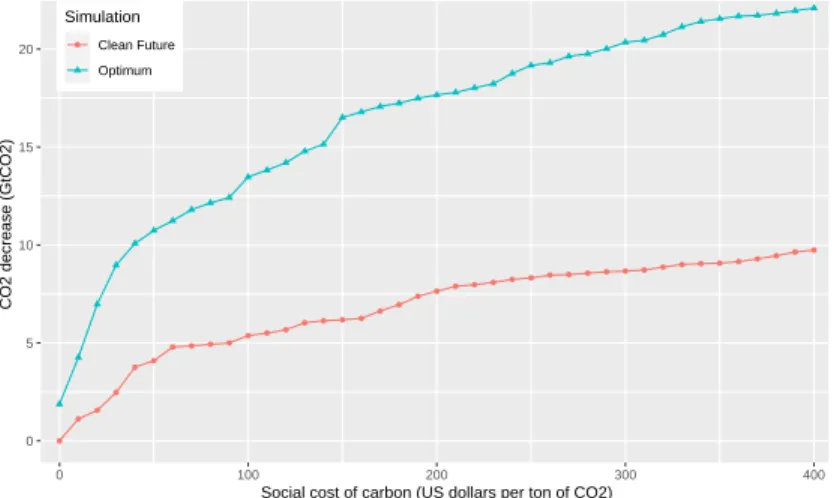
Missed opportunities and what can still be changed. We now look at the possible future gains from carbon pricing starting in 2019 (Clean future), compared to the baseline. Recall that the post-2019 baseline production minimizes the sum of discounted extraction costs. To determine the future supplies associated with the Clean future counterfactual and the baseline, we solve P1(T0 = 2019, Tf = 2050, µ) with µ = $200 and µ = $0, respectively.
We find emissions that are 7.64 GtCO2 lower in the Clean future with associated social gains
of 0.99 trillion US$: see the first two columns and the second row in Table 1. These results call for three comments. First, despite the lower future demand, factoring pollution costs in when deciding on future oil extraction will bring large environmental benefits, valued at 1.52 trillion US$, that come with an increased private cost of about 0.53 trillion US$
(= 1.52 − 0.99). This reflects that reserves as of 2019 are abundant and differ significantly in their private extraction costs and carbon intensities. Second, this reduction of 7.64 GtCO2 is
close to the 6.66 GtCO2 reduction over the same period (2019-2050) obtained when optimal
recomposition starts in 1992. In other words, the correction of carbon misallocation in the past would not preclude the large gains from the recomposition of current and future supply. This reflects that lower-carbon emission oil is relatively abundant. The third, and related, comment is that future emission reductions are much lower than the emissions drop of 17.66 GtCO2 from carbon pricing starting in 1992. In other words, past environmental
mistakes remain significant even if the best oil assets are eventually used in the future in place of dirtier but cheaper oil. Again, as good resources are relatively abundant, the opportunity cost of using clean resources in the past is small and does not prevent large gains later on in the extraction sequence. The missed opportunities of carbon mitigation in the past are then truly lost.
Lower bound of the gains over 1992-2018. Now, what is the value of these missed opportunities, i.e. what would have been the “early-action gains” from starting optimal extraction in 1992 rather than 2019? These early-actions gains are the opportunities we missed irreversibly as they cannot be mitigated by post-2018 optimal extraction. They represent a lower bound of misallocation costs over the 1992-2018 period. We calculate them by decomposing the gains from optimal extraction over the whole 1992-2050 period as follows, denoting x∗ Z as the solution of P1(T0 = Z, Tf = 2050, µ): MC(µ, x∗1992,1992, 2050) = MC(µ, x∗1992,1992, 2050) − MC(µ, x∗2019,2019, 2050) | {z } Early-action gains + MC(µ, x∗ 2019,2019, 2050) | {z } future gains (8) These early-action gains amount to 7.82 trillion US$ (= 8.81 − 0.99), and the corresponding emissions gains are 10.02 GtCO2 (= 17.66 − 7.64). The wrong selection of assets over
1992-2018 was thus responsible for, at least, 10.02 GtCO2.
Figure3shows the emission reductions in the Optimum and Clean future counterfactuals as a function of the social cost of carbon (SCC). Emission reductions from supply recompo-sition rise with the SCC, but are very stable over a large SCC range. At $100, the emission reductions from the Optimum and the Clean future are about 3/4 of those from the main exercise with a $200 SCC. The misallocation due to the 1992-2018 period as defined in (8), represented by the gap between the two curves, is remarkably constant: it varies from 7 to 12.5 GtCO2 as the SCC rises from $50 to $400/tCO2. These results are important, as they
for a SCC figure as low as $50 and for the whole range of SCC discussed in the literature (see Appendix C.6).
Is imperfect competition the source of carbon misallocation? One striking result is that the Optimum scenario over the 1992-2050 period produces a lower total cost of 8.81 trillion US$ relative to the baseline (the first column and first row in Table 1), of which 5.28 trillion US$ corresponds to private extraction costs and 3.53 trillion US$ to environmental costs. The environmental gains come with large private economic gains. Do the lower extraction costs show that clean oil is also the cheapest? That there is little correlation between private extraction costs and carbon intensities for all reserves available in 1992, as can be seen in Figure 2(b), suggests that this is not so. To demonstrate more rigorously that solving extraction-cost misallocation alone is not the principal source of environmental gains, we consider another counterfactual in which private extraction costs are minimized over the whole time path, absent any carbon pricing, i.e. the solution of P1(1992, 2050, 0).
We label this counterfactual Minimal private costs. We then compare this counterfactual to the baseline. Calling xpc
dt the extraction of deposit d at time t in this counterfactual, we
calculate the social gains of the cost-effective supply as MC((µt), (x pc dt), 1992, 2050) ≡ 2050 X 1992 X d (cd+ θdµt)(˜xdt− x pc dt)e −r(t−2018)
with µt = 200er(t−2018) to account for pollution cost and its impact on CO2 emissions as
P2050
1992Pdθd(˜xdt− xpc). The social gains here appear in the third row of Table1: total costs
fall by 6.63 trillion US$, of which 6.26 trillion US$ refer to lower private extraction costs. The corresponding drop in carbon emissions is only 1.87 GtCO2, i.e. about 10% of the Optimum
figure. Overall, carbon misallocation has little to do with cost misallocation. Comparing the social gains in the Optimum and the Minimal private costs counterfactuals (the first and third lines in the first column of Table 1), the specific gains from taking pollution into account instead of only minimizing private extraction costs amount to 2.18 trillion US$ (= 8.81 − 6.63).
Extraction order and the selection of resources. We know that the optimal pro-duction path differs from the baseline in two dimensions: the selection of resources and the extraction order. As far as pollution is concerned, the only way to reduce misallocation is to change some deposit’s cumulative extraction as compared to the baseline, i.e., to extract more of the ’good’ resources (that are not used, or not used enough, in the baseline) so as to avoid or reduce the use of ’bad’ resources. Part of the misallocation in private extraction costs is also explained by the extraction of the wrong deposits in the past, and some from the wrong ordering of deposit use. To pin-down the cost of this wrong order, we consider an
alternative counterfactual in which the recomposition of supply is limited to deposit reshuf-fling (Baseline reshufreshuf-fling). More precisely, we solve P1(1992, 2050, 0) under the constraints
that PTf T0 xdt =
PTf
T0 ˜xdt for all deposits d. Under this counterfactual, the cumulative
extrac-tion by deposit is left unchanged (as compared to the baseline) so that there is no possible environmental gain. The economic gain from this reordering is 4.65 trillion US$, over 88% of the gain in private extraction costs of 5.28 trillion US$ under the optimal counterfactual. The main source of extraction-cost misallocation can then be understood as the wrong order of asset use, whereas carbon misallocation only comes from the wrong selection of assets.
Feasibility constraint and other market failures. It can be argued that the envi-ronmental gains from the optimal extraction sequence would be difficult to obtain in practice as other sources of misallocation, such as market power, work in the opposite direction, or because countries would refuse to correctly price their domestic emissions were doing so to be to the detriment of their domestic oil industry.
We first address this issue in another counterfactual that constrains annual production in each OPEC member country to be equal to their historical value over the 1992-2018 period.21 The results appear in the third and fourth columns of Table 1. Maintaining the
annual productions of each OPEC country does not prevent significant emission reductions. We find environmental gains of carbon pricing of 17.78 GtCO2, valued at 3.56 trillion US$:
these are even slightly larger than the environmental gains estimated without the OPEC constraint. This constraint reduces total gains via increased private extraction costs: the gain in extraction costs falls to 3.53 trillion US$ (= 7.09−3.56), compared to 5.28 trillion US$ without the constraint.22 Second, the difference between this constrained counterfactual and
the optimum, which can be interpreted as the loss from OPEC’s market power, is 1.72 trillion US$. By way of comparison, the difference between the optimum and the counterfactual that minimizes private extraction costs (absent any environmental costs) without the OPEC constraint is 2.18 trillion US$. This last difference can be interpreted as the gain from carbon pricing.23 The gains from the removal of these two distinct market failures — imperfect
competition and carbon misallocation — are of the same magnitude.
Supply recomposition can lead to large welfare changes across countries. Although the winners from optimal supply recomposition could in theory compensate adversely-affected countries, this compensation is politically difficult to establish. Countries may have a
pref-21We abstract from market-power considerations after 2018, as the recent literature has argued that
OPEC market power has been considerably reduced (Huppmann and Holz,2012) and modeling oil-market
power is beyond the scope of this paper.
22The discounted profit of the OPEC over the 1992-2018 period increases in the optimum counterfactual,
which partly alleviates political feasibility issues.
erence for domestic production, for job-related, public-finance or energy-security reasons. These preferences may explain part of the cost misallocation we identify. In addition, coun-try preferences may pose a problem of feasibility for any ambitious supply reallocation. We thus re-run our main exercise constraining counterfactual annual production in each country to either match observed production or to be greater than the minimum of their production and consumption in two distinct exercises.24 The results are shown in Appendix
Table F1. Recomposing supply still produces large social gains and emission reductions. When country-level productions are kept at their baseline levels (the last two columns), the emission reductions compared to the baseline are 17.21 GtCO2, almost the same as the
17.66 GtCO2in the optimal counterfactual. In contrast, overall social gains fall to 6.28 (from
8.81 in Table1), representing lower private economic gains of about 2.44 US$ trillion, from a figure of 5.28 US$ trillion (= 8.81-17.66*0.2: the economic gains from the optimum without the constraint in Table 1) to 2.84 US$ trillion (= 6.28-17.21*0.2: the economic gains with the constraint in Appendix TableF1). Within-country private-cost misallocations therefore account for about 54% of total extraction-cost misallocation (= 2.84/5.28). This is in line with the estimates in Asker et al. (2019) for the 1970-2014 period. While CO2 total
abate-ment is stable, the private economic gains are significantly reduced by the country-specific constraints. This reveals that there is relatively more within-country variation in carbon intensities than in private extraction costs.
4.2
Sensitivity analysis
Appendix Table F2 tabulates the estimated gains and emission reductions from a series of counterfactual productions when we change our model parameters. Postponing the end of the oil era to 2066 has a large positive impact on the gains from implementing carbon pric-ing in 2019 instead of never (Clean future), mostly because this implies a greater demand to satisfy in the future in both the baseline and the counterfactual. On the contrary, it has a relatively limited impact on the overall gains and emission reductions from starting supply recomposition in 1992. There are two elements to extending the time horizon. First, the greater the demand, the more opportunities there are to improve the baseline. Second, oil abundance is reduced: were oil demand sufficient to exhaust all deposits, supply recompo-sition could not generate environmental gains. With a time horizon of 2066, the first effect continues to dominate, with environmental gains over the whole path that are larger than with a 2050 time horizon. This is still the case if we postpone the end of oil even further. Setting this to 2080 produces larger environmental gains, while reducing the economic gains.
24This also implies that variations in oil-transportation costs between the new counterfactual and the