Competition and water stress indices as predictors of Pinus halepensis Mill. radial growth under drought

HAL Id: hal-02523144

https://hal.inrae.fr/hal-02523144

Submitted on 6 Apr 2020

HAL is a multi-disciplinary open access

archive for the deposit and dissemination of

sci-entific research documents, whether they are

pub-lished or not. The documents may come from

teaching and research institutions in France or

abroad, or from public or private research centers.

L’archive ouverte pluridisciplinaire HAL, est

destinée au dépôt et à la diffusion de documents

scientifiques de niveau recherche, publiés ou non,

émanant des établissements d’enseignement et de

recherche français ou étrangers, des laboratoires

publics ou privés.

Competition and water stress indices as predictors of

Pinus halepensis Mill. radial growth under drought

Manon Helluy, Bernard Prévosto, Maxime Cailleret, Catherine Fernandez,

Philippe Balandier

To cite this version:

Manon Helluy, Bernard Prévosto, Maxime Cailleret, Catherine Fernandez, Philippe Balandier.

Com-petition and water stress indices as predictors of Pinus halepensis Mill. radial growth under drought.

Forest Ecology and Management, Elsevier, 2020, 460, pp.117877. �10.1016/j.foreco.2020.117877�.

�hal-02523144�

1

Competition and water stress indices as predictors of Pinus halepensis Mill. radial growth

1

under drought

2

Manon HELLUY1,2,3_{*, Bernard PREVOSTO}1_{, Maxime CAILLERET}1_{, Catherine FERNANDEZ}2_{, Philippe}

3

BALANDIER4

4

5

1 _{Irstea UR RECOVER, 3275 Route de Cézanne, F-13182 Aix-en-Provence, France}

6

2 _{IMBE, Aix Marseille Université, Avignon Université CNRS, IRD, UMR 7263, 3 place Victor-Hugo, F-13331}

7

Marseille cedex 3, France

8

9

4 _{Irstea, U.R. Forest Ecosystems, Domaine des Barres, F-45290 Nogent-sur-Vernisson, France}

10

11

*corresponding author

12

13

E-mail addresses: manon.helluy@irstea.fr (M. Helluy) ; bernard.prevosto@irstea.fr (B. Prévosto), maxime.cailleret@irstea.fr

14

(M. Cailleret); catherine.fernandez@imbe.fr (C. Fernandez); philippe.balandier@irstea.fr (P. Balandier)

15

16

17

18

19

20

21

22

23

24

25

26

27

28

29

Declaration of interest: none.

2

Abstract

31

The frequency, duration, and severity of drought events are expected to increase in the Mediterranean

32

area as a result of climate change, with strong impacts on forest ecosystems and in particular individual tree growth.

33

Tree growth response to drought is strongly influenced by local site and stand characteristics that can be quantified

34

using competition indices (CIs) and water stress indices (WSIs). These indices have been widely used to predict

35

tree growth; however, they are numerous, and few studies have investigated them jointly. In this context, we

36

investigated the potential of using CIs and WSIs to investigate tree behaviour under drought. The main objective

37

of this study was to quantify P. halepensis Mill. annual radial growth using tree size from the previous year, CIs

38

and WSIs.

39

We studied twelve 50-year-old Pinus halepensis plots located in the South-East of France distributed in

40

different density treatments (light, medium and dense). At each plot, all trees were measured (height,

41

circumference), spatialized and the ring-widths were measured for ~15 trees. We also developed a two-strata (over-

42

and understorey) forest water balance model to simulate soil water content at a daily resolution based on stand

43

characteristics (LAI values in particular) and soil properties. A mixed modelling approach was eventually used to

44

investigate the drivers of P. halepensis annual radial growth and to test the performance of five CIs and four WSIs.

45

The best growth model included tree size, the sum of Basal Area of Larger trees in a 5m-radius (BAL;

46

as CI), and the number of days that trees experienced water stress in a year (as WSI) as predictors. This model

47

explained up to 56 % of the variance in observed pine tree growth, which increased up to 77% when the individual

48

tree was included as a random effect on the intercept. We found that distance-independent CIs can perform as well

49

as distance-dependent CIs in our study site. The duration of drought alone appeared to better predict tree growth

50

than drought intensity and duration, or drought timing. The selected model led us to reaffirm the positive effect of

51

thinning on tree secondary growth when facing long and intense drought.

52

53

54

55

56

Radial growth; competition; water stress; Pinus halepensis; Mediterranean forests; model

57

58

59

3

1. INTRODUCTION

60

61

Drought has been identified as the main concern for the current and future functioning of Mediterranean

62

forest ecosystems (Peñuelas et al., 2017). It strongly impacts the physiological functions of Mediterranean tree

63

and shrub species, limiting their annual growth (Barbeta et al., 2015; Borghetti et al., 1998; Gazol et al., 2018;

64

Ogaya et al., 2003). Drought can also induce individual tree mortality and forest dieback in cases of long-term or

65

extreme drought events (Allen et al., 2010; Carnicer et al., 2011; Greenwood et al., 2017; Hayles et al., 2007).

66

Climate models project an increase in temperature – leading to increased potential evapotranspiration – combined

67

with a decrease in precipitation for the Mediterranean area (Giorgi, 2006). This will likely lead to an increase in

68

the duration, intensity and frequency of droughts (Cramer et al., 2018). In this context, understanding the processes

69

underlying the response of trees to drought is not only important for fundamental knowledge, but also for forest

70

management. Some forest management strategies have already been proposed to enhance Mediterranean forests’

71

growth productivity under dry conditions and to adapt them to climate change, in particular through the reduction

72

of competition among trees by thinning (Aldea et al., 2017; Bréda et al., 1995; Calev et al., 2016; Sohn et al.,

73

2016; Vilà-Cabrera et al., 2018).

74

Ecological competition is defined as a negative interaction between plants, which can be direct (direct

75

contact, allelopathy) or indirect through the use of common resources (Connell, 1990), and can be intraspecific or

76

interspecific. Thus, competition defines the pattern of net resource availability and is largely responsible for

77

differences in individual growth among trees with varying social status and neighbourhoods (Calama et al., 2019).

78

Competition is considered symmetric when competitors share resources in proportion to their size, while

79

competition is considered to be asymmetric when large competitors capture a disproportionate share of contested

80

resources over smaller competitors (Schwinning & Weiner, 1998). On one hand, trees’ modes of competition are

81

driven by environmental factors and are linked to the most prevailing limiting factor (limitation-caused matter

82

partitioning hypothesis; Pretzsch & Biber, 2010). Competition for belowground resources is often assumed to be

83

symmetric – like in water-limited ecosystems (Pretzsch & Biber, 2010) e.g. Mediterranean ecosystems – while

84

competition for light is asymmetric due to the directional component of light (Schwinning & Weiner, 1998). On

85

the other hand, competition also modulates individual tree response to drought. For example, the reduction of

86

competition by thinning tends to increase stand-level water availability (Bréda et al., 1995) and may alleviate

87

drought-related reductions in tree growth (e.g., Aldea et al., 2017; Gavinet et al., 2015; Olivar et al., 2014; Sohn

88

et al., 2016). In addition, trees can have various responses to drought depending on the species, their size and

4

90

(Castagneri et al., 2012; Sánchez-Salguero et al., 2015; Zang et al., 2012) while other studies have found the

91

opposite pattern (Calama et al., 2019; Martin-Benito et al., 2011; Trouvé et al., 2017) or no difference between

92

dominant and suppressed trees (Bello et al., 2019; Lebourgeois et al., 2014). These contrasting results can be

93

explained by species-specific differences in shade- and drought-tolerance strategies, and by differences in the

94

population and site characteristics, especially in the stand water balance, whose spatiotemporal dynamics is often

95

not well quantified or considered.

96

Considering the various relationships between competition and drought and their impacts on tree radial

97

growth, models that aim to accurately predict individual tree growth or stand-scale productivity should take into

98

account both competitive and climatic drivers at an annual resolution (Ameztegui et al., 2017). Including these

99

drivers is important to correctly simulate (i) decadal and multi-decadal growth trends, which are strongly

100

influenced by competition, (ii) the impacts of human and natural disturbances on the spatial arrangement of the

101

stand and on the competition intensity experienced by each tree (e.g. after thinning or massive mortality), and (iii)

102

the interannual variability in tree growth, which is mainly controlled by interannual climate variability (Calama et

103

al., 2019; Condés & García-Robredo, 2012; Rathgeber et al., 2005; Sánchez-Salguero et al., 2015). This is

104

especially important to improve empirical forest growth models that statistically link growth data with specific site

105

and climatic conditions. Though empirical models are difficult to extrapolate, they are very precise under their

106

calibration domain and are widely used for forest management planning (e.g. growth and yield models; see

107

Weiskittel Jr et al., 2011).

108

Several types of indices can be used in such empirical forest growth models to assess the competition and

109

water stress experienced by a tree. Competition indices are often used to investigate the different modes of

110

competition (Biging & Dobbertin, 1995; Prévosto, 2005). For example, asymmetric competition for light can be

111

predicted using competition indices that derive from tree heights and crown sizes, while symmetric competition

112

for belowground resources can be predicted using competition indices based on tree diameters, root mass, or

113

rooting depths (Pretzsch et al., 2017). Many drought indices have been developed for modelling purposes. Speich

114

(2019) classified these drought indices into four levels, from the least to the most integrative: (1) based on

115

precipitation, (2) based on evaporative demand, (3) based on soil moisture storage and stand properties, and (4)

116

based on physiological thresholds. Drought indices that are more mechanistic generally perform better at

117

predicting tree growth than indices including precipitation and evaporative demand, or precipitation alone (Speich,

118

5

119

experienced (4).

120

In this study, we developed an empirical mixed modelling approach to predict individual Aleppo pine

121

(P.halepensis Mill.) radial growth based on its size, neighbourhood, and climatic factors. We used five competition

122

indices (CIs) that are derived from different types of information in order to investigate the modes of competition

123

of P.halepensis. Several water stress indices (WSIs), with contrasting levels of information were also used to

124

investigate the influence of water stress induced both by soil and climatic factors on P.halepensis radial growth.

125

We especially aimed at evaluating the potential of competition indices (CIs) and water stress indices (WSIs) jointly

126

for predicting annual basal area increment (BAI) in Pinus halepensis under different thinning intensities, and

127

selecting the best CI and WSI indices. Our main hypothesis were, as follows:

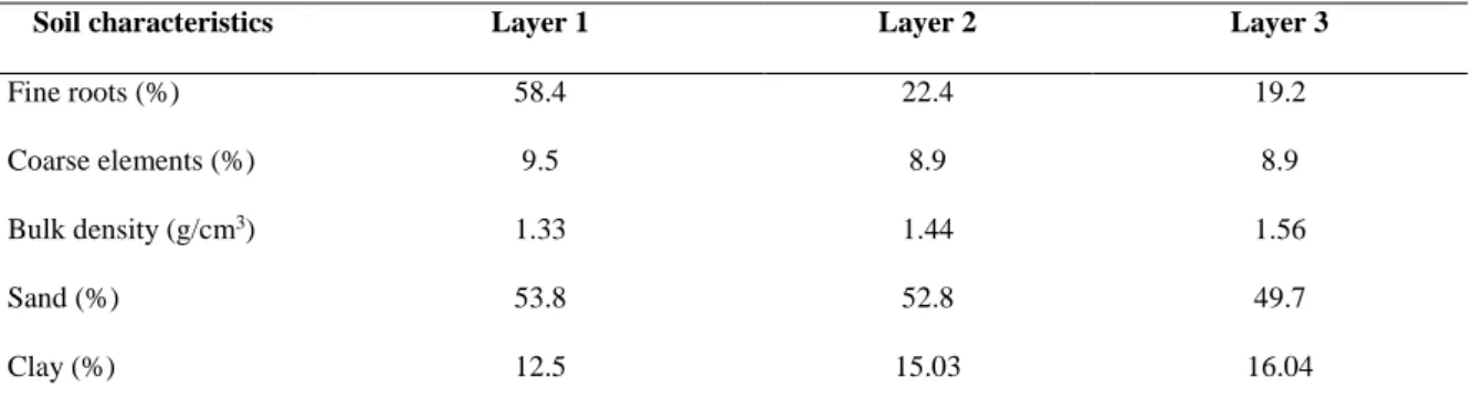
128

(i) P.halepensis’ main mode of competition is symmetric;

129

(ii) Soil water availability is a better predictor of P.halepensis growth than rainfall alone;

130

(iii) The best pine growth model includes both competition indices and water stress indices.

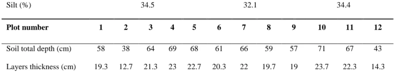
131

132

2. MATERIAL AND METHODS

133

2.1. Study site and experimental design

134

135

This study was conducted in Southern France in the ‘Saint Mitre’ experimental site, which is located

136

about 30 km west of Marseille (43°27’0”N; 5°2’24”E). The area is flat and at a mean altitude of 130 m above sea

137

level. The climate is Mediterranean, with warm, dry summers and cool, wet winters. The mean annual temperature

138

is 15.3°C and mean annual precipitation is 562 mm (Istres weather station, 1985-2014; Appendix A). However,

139

fluctuations in rainfall are frequently observed between years. For example, 2015 and 2016 received 660 mm and

140

411 mm of rainfall, respectively. Soils are calcareous, with a sandy-loam texture (55% sand, 30% silt and 15%

141

clay) and a mean depth of 60 cm before reaching the calcareous bedrock. The site is composed of a monospecific

142

even-aged (~60 years old) Aleppo pine forest (Pinus halepensis Mill.) that has naturally regenerated after

143

agricultural abandonment ~60 years ago. The understorey is mainly composed of Mediterranean oaks (Quercus

144

ilex and Quercus coccifera), shrubs (e.g. Phillyrea angustiflia, Rosmarinus officinalis) and scarce herbaceous

145

plants (e.g. Brachypodium retusum).

146

Natural pine stands were thinned in 2007, leading to three different pine cover treatments and thus

147

different competition situations: (i) light pine cover (basal area: 10.2 m².ha-1_{), (ii) moderate pine cover (19.2}

6

149

(Appendix B). All pines were individually identified, geo-referenced in spring 2017 using a differential GPS

150

(Trimble© TSC2, Trimble Inc, USA) and a laser distance meter (LaserAce® 300, Measurements Devices Ltd,

151

UK). Their circumference at breast height (1.30m) and their height were measured in 2017 using a measuring tape

152

and a rangefinder (Vertex III, Häglof, Sweden), respectively.

153

154

2.2. Measurement of individual tree growth based on ring-width series

155

156

From September to October 2017, 1-2 cores were extracted at breast height using a Pressler increment

157

borer from 15 randomly selected (co-)dominant Aleppo pines in the inner part of each of the 12 plots (20m*20m,

158

to reduce border effect, Appendix C). Cores were mounted and sanded until ring boundaries were clearly visible.

159

We used the WinDENDRO program (WinDENDROTM _{2014, © Regent Instruments Canada Inc.) to measure ring}

160

widths at a resolution of 0.034 mm and visually cross-date each individual chronology. We removed the series

161

that could not be accurately cross-dated (e.g. due to high polycyclism rate and/or high number of missing rings).

162

Most of the removed trees were in the dense cover treatments, however at the end the distribution of individuals

163

within the treatments was even (dense cover: 62 individuals; moderate cover: 58 individuals; light cover: 55

164

individuals). In order to have a single series per tree, chronologies were averaged for each individual tree when

165

two of them were available. This resulted in 175 individual tree-ring width series that were retained for the

166

following analyses.

167

To correct the trend associated with the geometrical constraint of adding a volume of wood to a stem of

168

increasing radius, the tree-ring width series were converted into basal area increments (BAI) (Biondi & Qeadan,

169

2008) using the following formula:

170

171

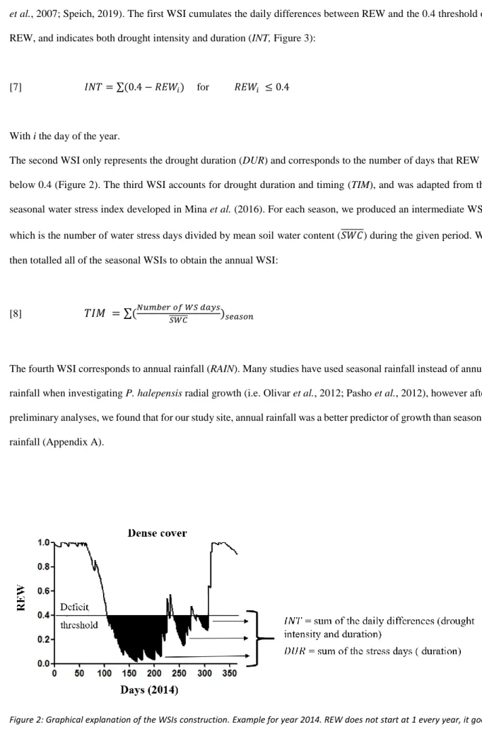
[1] 𝐵𝐴𝐼 = 𝜋(𝑟𝑡2− 𝑟𝑡−12 )

172

173

With 𝑟𝑡2 and 𝑟𝑡−12 referring to the stem radii corresponding to years t and t-1, respectively.

174

The BAI was then used to represent the annual individual tree growth. Only the data from 2008 to 2017 were used

175

for the analyses, as the structure of the thinned stands was not known before that date.

176

177

178

7

179

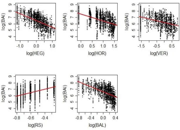
2.3. Selection of the competition indices

180

181

Competition was quantified using competition indices (CIs). CIs can also be classified into two

182

categories: distance-dependent CIs based on the relative dimensions and the distance of a subject tree to its

183

neighbours within a given radius; and distance-independent CIs based only on non-spatial and aggregated

184

information on tree size and the number of trees in a given area. We used 5 different CIs based on the literature,

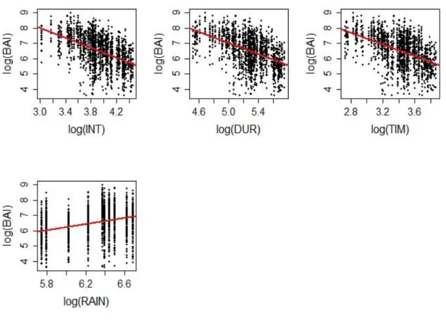
185

using different types of information (distance, circumference, height) in order to compare their predictive power

186

and to investigate the dominant mode of competition (symmetric or asymmetric). In this study, we tested three

187

distance-dependent indices (HEG to VER), and two distance independent indices (RS and BAL). The first CI (HEG)

188

is a distance weighted size-ratio index, developed by Hegyi (1974). Because it uses tree circumferences, it is

189

expected to account for symmetric competition:

190

191

𝐻𝐸𝐺 = ∑

192

193

Ci is the circumference at breast height of the subject tree i, Cj is the circumference of the neighbour tree j, and

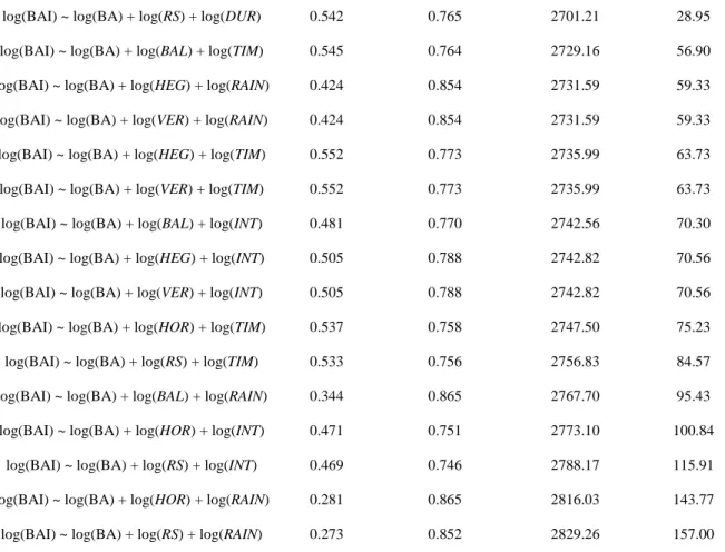
194

dist is the distance between both trees i and j.

195

The second and third indices were developed by Pukkala & Kolström (1987). They are based on the sum of

196

horizontal or vertical angles that originate from the subject tree, spanning the circumference or the top of the crown

197

of each neighbour tree (HOR and VER), respectively. HOR is based on the circumferences of all neighbours, and

198

is expected to account for symmetric competition. In contrast, VER uses the height of taller neighbours and is

199

expected to account for asymmetric competition:

200

201

𝐻𝑂𝑅 = ∑

2. arctan (

)

202

203

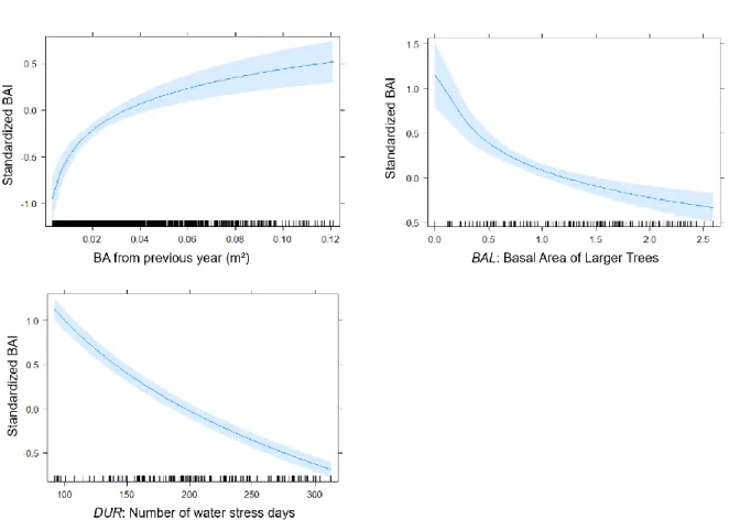
𝑉𝐸𝑅 = ∑

arctan (

)

204

8

205

The fourth index is the Relative Spacing (RS) index developed by Schröder & Gadow (1999). This index is

206

computed at the plot scale, which leads to a single plot-level value:

207

208

𝑅𝑆 =

)

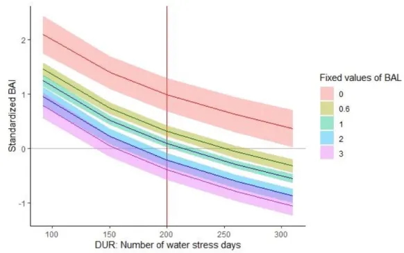
209

210

With N the number of stems per hectare and Hd the dominant stand height. The dominant stand height is usually

211

defined as the height of the 100 tallest trees in one hectare; however for our study we took the 5 tallest trees in

212

each plot.

213

The last index was first developed by Wykoff et al. (1982), and corresponds to the total basal area of trees that are

214

larger than the subject tree (also called Basal Area of Larger trees; BAL). It is expected to account for asymmetric

215

competition as only large trees are taken into account, but also for symmetric competition, as it is size-related:

216

217

𝐵𝐴𝐿 = ∑

218

219

We computed the values of the distance-dependent competition indices (HEG, HOR, VER) for different

220

competition radii (from 1 meter to 8 meters), and then calculated the correlation coefficients between the mean

221

BAI for 10 years and the competition index. We then selected a competition radius of 5 meters for the three

222

distance-dependent indices (see Appendix D). In total, we produced five competition indices for each individual

223

tree. We did not have height and circumference data for all individual trees between 2008 and 2017, but as the

224

stands are quite homogeneous and major changes in the stand composition and structure did not occur between

225

2007 and 2017 (Appendix F) we made the very likely assumption that individual CIs remained constant over this

226

period.

227

228

2.4. Water Balance model

229

230

The effects of the climate, stand, and soil properties on drought characteristics can be integrated into a

231

forest water balance model. We thus developed a two-strata forest water balance model, i.e. over- and understorey

232

9

233

et al., (1999), which computes daily variations in soil water content. The model uses daily temperatures and rainfall

234

data as inputs, and some site and stand parameters such as soil depth, maximum and minimum extractable soil

235

water (from soil texture analyses), fine root distribution, soil porosity, and stand Leaf Area Index (LAI). Istres

236

weather station (12 km NW of the site) provided the climatic data over the entire study period and global radiation

237

data came from Marignane station (14km E of the site). The PET was computed using the radiation-based method

238

of Turc (Turc, 1961) in the absence of wind data recorded on-site. Soil samples were collected in 2014 and 2017.

239

In 2014, 2 plots per treatment were sampled; in each of the selected plots 6 soil samples at three soil depths were

240

collected for texture analysis. In 2017, 5 soil pits were dug into the treatments and 30 soil samples of constant

241

volume (3 soil depths and 2 samples per depth) were collected to measure the bulk density, the content in coarse

242

elements and in fine roots (Table 1). The soil properties were considered as constant among the plots, except for

243

soil depth. Water buckets were computed for each soil layer (Jabiol et al., 2009) and aggregated at the plot scale.

244

Transmitted radiation was measured every minute for 48 hours during two successive clear days of April 2017 in

245

9 plots (3 plots/treatment) using 6 solarimeter tubes (PAR/LE Solems) per plot and 2 solarimeter tubes in open

246

conditions, in order to compute transmitted radiation. Based on this transmitted radiation, LAI was then calculated

247

using the Norman & Jarvis (1975) equations. A relationship between stand basal area and the LAI values was

248

established to model the changes of LAI through time. The LAI was later used to compute the rainfall interception

249

of the Aleppo pine canopy and the understorey using the model proposed by Molina & del Campo (2012). Rainfall

250

interception, transpiration of the two strata, and the soil water dynamics were computed and provided daily

251

variations of soil water content and relative extractable water (Prévosto et al., 2018) (REW, daily extractable water

252

standardized by maximum water extractable; Figure 1).

253

254

Table 1: Soil characteristics incorporated for each layer of each plot in the water balance model. Only variations

255

in layer thickness was incorporated within plots.

256

Soil characteristics Layer 1 Layer 2 Layer 3

Fine roots (%) 58.4 22.4 19.2 Coarse elements (%) 9.5 8.9 8.9 Bulk density (g/cm3_{) 1.33 1.44 1.56}

Sand (%) 53.8 52.8 49.7

10

Silt (%) 34.5 32.1 34.4

Plot number 1 2 3 4 5 6 7 8 9 10 11 12

Soil total depth (cm) 58 38 64 69 68 61 66 59 57 71 67 43 Layers thickness (cm) 19.3 12.7 21.3 23 22.7 20.3 22 19.7 19 23.7 22.3 14.3

257

258

Figure 1: Variations in rainfall, potential evapotranspiration (PET) and relative extractable water (REW) calculated using the

259

water balance model from between 2008 and 2017.

260

2.5. Water stress indices (WSI)

261

262

For each plot and each year, we used four different WSIs using different levels of information i.e. soil

263

and/or climatic constraints. The first three WSIs derive from the forest water balance to account for climate and

264

local conditions, while the fourth WSI derives directly from climatic data. We assumed that a drought had occurred

265

when the soil REW dropped below a threshold of 0.4, as proposed by Granier et al. (1999), a threshold that has

266

been successfully applied in other empirical and modelling studies (Bello et al., 2019; Forner et al., 2018; Granier

267

11

et al., 2007; Speich, 2019). The first WSI cumulates the daily differences between REW and the 0.4 threshold of

268

REW, and indicates both drought intensity and duration (INT, Figure 3):

269

270

[7] 𝐼𝑁𝑇 = ∑(0.4 − 𝑅𝐸𝑊𝑖) for 𝑅𝐸𝑊𝑖 ≤ 0.4

271

272

With i the day of the year.

273

The second WSI only represents the drought duration (DUR) and corresponds to the number of days that REW is

274

below 0.4 (Figure 2). The third WSI accounts for drought duration and timing (TIM), and was adapted from the

275

seasonal water stress index developed in Mina et al. (2016). For each season, we produced an intermediate WSI,

276

which is the number of water stress days divided by mean soil water content (𝑆𝑊𝐶) during the given period. We

277

then totalled all of the seasonal WSIs to obtain the annual WSI:

278

279

[8]

𝑇𝐼𝑀 = ∑(

)

280

281

The fourth WSI corresponds to annual rainfall (RAIN). Many studies have used seasonal rainfall instead of annual

282

rainfall when investigating P. halepensis radial growth (i.e. Olivar et al., 2012; Pasho et al., 2012), however after

283

preliminary analyses, we found that for our study site, annual rainfall was a better predictor of growth than seasonal

284

rainfall (Appendix A).

285

286

287

288

Figure 2: Graphical explanation of the WSIs construction. Example for year 2014. REW does not start at 1 every year, it goes

289

on from year to year.

12

291

is thus expected to be sensitive to cold temperatures, which could negatively affect its growth. However, such

292

temperatures are not seen at our study site (Appendix A). Secondly, during preliminary analyses, annual minimum

293

and maximum temperatures were found to be poor predictors of tree growth and were thus removed from the final

294

analyses (Appendix D).

295

296

2.6. Statistical analyses, growth models and indices selection

297

298

Kruskal-Wallis non-parametric tests followed by Dunn’s test were performed to explore the effect of the

299

cover treatments on BAI, using the {dunn.test} package (Dinno, 2017) from the open-source R statistical software

300

(R Core Team, 2017).

301

Simple linear regressions were used to explore the relationships between tree BAI and the different

302

CIs/WSIs. To jointly test the influence of both competition and water stress on P. halepensis tree growth, we

303

developedlinear mixed-effect models using the {lme4} and {lmerTest} packages (Kuznetsova et al., 2017). Natural

304

logarithm transformations were used to satisfy the assumptions of linearity and normality of the residuals, the

305

‘LogSt’ function from the {DescTools} package (Signorell et al., 2019) being specifically used to account for null

306

CI values. This led to the following model equation:

307

308

[9] log(𝐵𝐴𝐼𝑖,𝑡) = 𝑘 + ∝ log(𝐵𝐴𝑖,𝑡−1) + 𝛽 log(𝐶𝐼𝑖) + 𝛾 log(𝑊𝑆𝐼𝑡) + 𝛿𝑖 + 𝜀

309

310

Where k, ∝, β and γ are the fixed parameters, BAIi,t the basal area increment (mm²) of the tree i during the year t,

311

BAi,t-1 the tree basal area of previous year t-1 (m²), CIi, a competition index, WSIt a water stress index of the year

312

t, i the random effect estimated for the intercept with tree as a grouping factor, and  is the residual error. BA was

313

included in the models to account for the effect of tree size on current annual growth. We included trees nested

314

into the plot, plots alone, or trees alone as a random effect on the intercept term; however after preliminary analysis

315

we retained the tree random effect alone as it performed better. Similarly, we added a tree random effect on the

316

parameters (slope), however all of these random effect models failed to converge. Finally, the tree random effect

317

on the intercept term was the only to be retained. We also investigated the interaction between competition and

318

water stress, but the interaction was not significant and only the additive models were retained.

319

13

320

and WSI were selected using the Akaike’s Information Criterion (AIC) with maximum likelihood fitting (MLE)

321

as only our fixed effects differed between models. The parameters of the best model were fitted using restricted

322

maximum likelihood (REML). We used the marginal r-squared (variance explained by the fixed effects only) and

323

the conditional r-squared (variance explained by both fixed and random effects) using the R package {MuMIn}

324

(Barton, 2018) as indicators of model performance. The marginal r-squared of the best model were bootstrapped

325

using the R package {boot} to produce confidence intervals and to evaluate the model’s robustness (Canty &

326

Ripley, 2019; Davison & Hinkley, 1997). The bootstrap was stratified (strata: individual tree) and based on 2000

327

replicates. Conditional r-squared were not used for the bootstrap, as this method does not correctly estimate the

328

variance in a random effect model, in particular when the variables are not independent and identically distributed

329

(McCullagh, 2000).The normality of the residuals and multicollinearity of the explanatory variables were tested

330

using Shapiro-Wilk test and the Variance Inflation Factor, respectively. To evaluate the effect of the selected

331

variables on the standardized-BAI, effect plots were produced using the R package {effect} (Fox & Weisberg,

332

333

334

335

3.1. Temporal variability in tree BAI

336

337

Over the 2008-2017 study period, there was a consistent increasing gradient of BAI from the control to

338

the light cover treatment (Figure 3), confirmed by the Kruskal-Wallis test and Dunn’s test: significant differences

339

were found between the three treatments for all years (Kruskal-Wallis statistics: Chi square = 466.99, df = 2,

p-340

value < 2.2e-16_{). There was high variability between years with 2016 and 2017 being the least productive years.}

14

342

Figure 3: Variations of tree basal area increment (BAI ; mm²) between 2008 and 2017 among the cover treatments resulting

343

from different thinning intensities (Dense, Moderate, Light). Medians, 1st _{and 3}rd _{quartiles are presented. Decline in growth}

344

in 2016 and 2017 is a climatic trend, these years being both extremely dry (411mm and 311mm, respectively).

345

346

3.2. Linear regressions with one-single explanatory variable

347

348

BAI was negatively correlated with the CIs 1, 2, 3 and 5 – indicating that the higher the competition

349

experienced by the tree is, the lower its growth rates are (Figure 4, r² from 0.218 to 0.377). On the contrary, when

350

RS increased (the relative spacing between trees), the BAI increased as well: the wider the spacing between trees

351

is, the greater the BAI is (r² = 0.209).

352

15

354

Figure 4: Tree Basal Area Increment (BAI) relative to Competition Indices (CIs). Curve fits in the graphs are separate linear

355

regressions, from HEG to BAL: log(BAI) = -1.063 log(HEG) + 6.517, r² = 0.377; log(BAI) = -1.078 log(HOR) + 7.520, r² = 0.228;

356

log(BAI) = -0.582 log(VER) + 6.200, r² = 0.218; log(BAI) = 2.657 log(RS) + 8.068, r² = 0.209; log(BAI) = -1.925 log(BAL) + 6.612,

357

r² = 0.291. All slopes are significantly different from zero (p < 0.001)

358

As indicated by the different linear regressions, there was a negative relationship between the BAI and

359

the WSIs (except for RAIN; Figure 5), which indicates that when the water stress increases, the BAI decreases (r²

360

from 0.248 to 0.260). In contrast, when rainfall increases (RAIN) the BAI increases as well, though the relationship

361

is weaker (r² = 0.101).

16

363

Figure 5: Tree Basal Area Increment (BAI) relative to Water Stress Indices (WSIs). Curve fits in the graphs are separate linear

364

regressions, from INT to RAIN: log(BAI) = -1.657 log(INT) + 13.020, r² = 0.255; log(BAI) = -1.813 log(DUR) + 16.074, r² = 0.260;

365

log(BAI) = -1.915 log(TIM) + 13.077, r² = 0.248; log(BAI) = 1.032 log(RAIN) + 0.049, r² = 0.101. All slopes are significantly

366

different from zero (p < 0.001)

367

368

3.3. Linear mixed-effects models with multiple explanatory variables: selection of the indices

369

370

For the single variable models, HEG (Hegyi competition index) and DUR (number of days that trees

371

experienced water stress) were the best explanatory indices (38% and 16% of the variance explained, respectively).

372

HEG and DUR were still the best predictors when BA was included in the mixed models (38% and 53% of the

373

variance explained by the HEG and DUR models, respectively). However, WSIs and BA combined were better

374

predictors of growth than CIs and BA together (RAIN excluded), the marginal R² ranged from 43% to 53% for the

375

WSIs and from 30% to 40% for the CIs, respectively. When three explanatory variables were included, the best

376

five models included BA, DUR and different variants of the CIs (Table 2). In the best model, BAL – sum of the

377

basal area of larger trees – and DUR – the number of water stress days – were selected together. The fixed effects

378

17

(0.516-379

0.576; obtained from bootstrapping), highlighting its low dependency on the characteristics of the input dataset

380

and its high robustness. Finally, the inclusion of the random effect considerably improved the models explaining

381

a large proportion of the remaining variance (e.g. 22% for the best model).

382

383

Table 2: Linear mixed-effects models of the annual tree basal area increment (BAI) as a function of the basal area of the

384

previous year (BA) and the different indices produced previously (CI and WSI). Selected models are in bold in their group; the

385

final selected model is in bold and red.

386

Models (with tree as a random effect on the intercept)

Marg. R² Cond. R² AIC ∆i

log(BAI) ~ log(HEG) 0.378 0.678 3438.12 0.00 log(BAI) ~ log(BAL) 0.291 0.677 3478.62 40.50 log(BAI) ~ log(VER) 0.229 0.677 3502.86 64.74 log(BAI) ~ log(HOR) 0.219 0.677 3506.58 68.46 log(BAI) ~ log(RS) 0.210 0.677 3509.45 71.33 log(BAI) ~ log(DUR) 0.161 0.776 2798.09 0.00 log(BAI) ~ log(INT) 0.154 0.770 2839.22 41.12 log(BAI) ~ log(TIM) 0.149 0.768 2853.73 55.64 log(BAI) ~ log(RAIN) 0.102 0.790 2893.81 95.72

log(BAI) ~ log(BA) + log(HEG) 0.376 0.899 3276.37 0.00

log(BAI) ~ log(BA) + log(BAL) 0.328 0.908 3303.17 26.79 log(BAI) ~ log(BA) + log(HOR) 0.305 0.929 3366.63 90.26 log(BAI) ~ log(BA) + log(VER) 0.309 0.931 3373.32 96.95 log(BAI) ~ log(BA) + log(RS) 0.304 0.935 3390.50 114.13

log(BAI) ~ log(BA) + log(DUR) 0.527 0.755 2704.38 0.00

log(BAI) ~ log(BA) + log(TIM) 0.516 0.745 2761.41 57.04 log(BAI) ~ log(BA) + log(INT) 0.434 0.719 2802.18 97.80 log(BAI) ~ log(BA) + log(RAIN) 0.125 0.877 2885.25 180.88

log(BAI) ~ log(BA) + log(BAL) + log(DUR) 0.556 0.773 2672.26 0.00

log(BAI) ~ log(BA) + log(HEG) + log(DUR) 0.561 0.781 2681.25 8.99 log(BAI) ~ log(BA) + log(VER) + log(DUR) 0.561 0.781 2681.25 8.99 log(BAI) ~ log(BA) + log(HOR) + log(DUR) 0.547 0.767 2691.22 18.96

18

log(BAI) ~ log(BA) + log(RS) + log(DUR) 0.542 0.765 2701.21 28.95 log(BAI) ~ log(BA) + log(BAL) + log(TIM) 0.545 0.764 2729.16 56.90 log(BAI) ~ log(BA) + log(HEG) + log(RAIN) 0.424 0.854 2731.59 59.33 log(BAI) ~ log(BA) + log(VER) + log(RAIN) 0.424 0.854 2731.59 59.33 log(BAI) ~ log(BA) + log(HEG) + log(TIM) 0.552 0.773 2735.99 63.73 log(BAI) ~ log(BA) + log(VER) + log(TIM) 0.552 0.773 2735.99 63.73 log(BAI) ~ log(BA) + log(BAL) + log(INT) 0.481 0.770 2742.56 70.30 log(BAI) ~ log(BA) + log(HEG) + log(INT) 0.505 0.788 2742.82 70.56 log(BAI) ~ log(BA) + log(VER) + log(INT) 0.505 0.788 2742.82 70.56 log(BAI) ~ log(BA) + log(HOR) + log(TIM) 0.537 0.758 2747.50 75.23 log(BAI) ~ log(BA) + log(RS) + log(TIM) 0.533 0.756 2756.83 84.57 log(BAI) ~ log(BA) + log(BAL) + log(RAIN) 0.344 0.865 2767.70 95.43 log(BAI) ~ log(BA) + log(HOR) + log(INT) 0.471 0.751 2773.10 100.84 log(BAI) ~ log(BA) + log(RS) + log(INT) 0.469 0.746 2788.17 115.91 log(BAI) ~ log(BA) + log(HOR) + log(RAIN) 0.281 0.865 2816.03 143.77 log(BAI) ~ log(BA) + log(RS) + log(RAIN) 0.273 0.852 2829.26 157.00

Abbreviations: Marg. R² the marginal r-squared (accounting for the fixed effects); Cond. R² the conditional r-squared

387

(accounting for the fixed and random effects); AIC the Akaike Information Criterion; ∆i the difference in AIC with respect to

388

the best fitting model of each category delimited by plain black lines.

389

390

Table 3: Estimated coefficients, standard errors (Std. errors) and p-values for the best model. The variances of 𝜀𝑟𝑎𝑛 and 𝜀𝑟𝑒𝑠

391

are shown as well.

392

log(𝐵𝐴𝐼𝑖,𝑡) = 𝑘 + ∝ log(𝐵𝐴𝑖,𝑡−1) + 𝛽 log(𝐵𝐴𝐿) + 𝛾 log(𝐷𝑈𝑅) 𝛿𝑖 𝜀

Parameters Estimates Std. errors P value Variance Variance

k 15.974 0.409 < 2e-16 * 0.206 0.212 α 0.410 0.064 6.29e-10 * β -1.027 0.175 1.94e-08 * γ -1.497 0.048 < 2e-16 * *significant correlation (p < 0.01)

393

394

19

3.4. Predicted effects of the main variables from the best model on growth

395

396

All of the variables of the best final model significantly affect individual BAI (Table 3). Basal area in the

397

previous year (BAt-1) had a positive effect on BAI (Table 3 & Figure 6). From 0.01 m² to approximately 0.04 m²,

398

BAt-1 had a strong positive effect on BAI. This positive effect became relatively lower with higher variability

399

between 0.04 m² and 0.10 m² due to sparse data. Both BAL and DURhad a negative effect on BAI overall. DUR

400

had a negative effect on BAI with low variability. BAL had a strong negative effect on BAI with high variability

401

between 0 and 1 and a more neutral negative effect on BAI with higher variability when BALranged between 1

402

and 3.

403

404

Figure 6: Predicted effects of BAt-1, BAL, and DUR on standardised BAI estimated using the best three-variable model (table 2).

405

Shaded areas around the curves represent the confidences intervals of the mean (95%). Straight lines above the x-axis

406

represent the distribution of the measured data.

407

The relationship between BAL and DUR is only additive, which means that pine growth response to

408

drought is the same under different levels of BAL. However, BAL reduces growth, i.e. the higher the BAL the

409

lower the growth (Figure 8). For example, when drought duration equals 200 days in a year, pine trees experiencing

410

no competition at all increase annual pine growth by 1mm², while pines experiencing strong competition (BAL =

411

20

412

number of water stress days pine trees can tolerate in a year before BAI is considerably affected (i.e. when

413

standardized BAI drops below 0). In our example, when BAL = 3, standardized BAI drops below 0 after 150 water

414

stress days. When BAL = 1, standardized BAI drops below 0 only after 200 water stress days. Finally, when BAL

415

= 0, standardized BAI never goes below 0 (Figure 8).

416

417

Figure 7: Predicted effects of the number of days with water stress (DUR) on standardised BAI according to different fixed

418

values of Basal Area of Larger trees (BAL; in colors), estimated using the best three-variables model (table 2). Shaded areas

419

around the curves represent the 95% confidences intervals of the mean effects (means are the coloured curves). The mean

420

standardized growth (horizontal line) and the value of DUR=200 is indicated in red (vertical line) (see also comments in the

421

422

423

424

425

In this study, the Hegyi competition index (HEG) was selected as the best predictor of individual annual

426

BAI among the competition indices for the one-variable and the two-variable models, followed by the basal area

427

of larger trees (BAL; BAL), the angles CIs (i.e. HOR and VER), and the relative spacing CI (RS). This suggests

428

that competition would mainly be symmetric, i.e. the system is limited by water. However, the BAL was selected

429

as the best predictor of BAI among the CIs in the three-variable models, followed closely by the Hegyi CI (HEG),

430

21

431

be taken into account by WSIs. In other words, this indicates that some CIs do indeed reflect the competition for

432

water. The poor performance of RS can be explained by its generality as it provides a single competition value for

433

all trees within a given plot, which does not accurately represent the actual competition experienced by each

434

individual tree.

435

The three best CIs (BAL, HEG and VER) correspond to three different methods of computing competition;

436

despite this, BAL, HEG and VERhave similar BAI predictive power, with a marginal r-squared of about 56%.

437

HEG only relies on circumference and should indicate symmetric competition for belowground resources, while

438

BAL also relies on circumferences but only incorporates trees larger than the subject tree, reflecting both

439

asymmetric and symmetric competition. VER uses tree height, which is more subject to measurement errors, but

440

is more representative of competition for light (e.g. asymmetric competition) than circumference. We investigated

441

the relationship between height and circumference. However, no clear relationship was detected (Appendix G),

442

indicating that both represent different aspects of competition with water stress indices explaining yet another

443

aspect of competition. It also highlights the fact that CIs can share some information, as competition can never be

444

defined as completely size-symmetric or completely size-asymmetric (Schwinning & Weiner, 1998). Hence, our

445

hypothesis (i) is not entirely verified: P.halepensis’ mode of competition seems to be asymmetric, but this is

446

contradicted by the good performance of the HEG index.

447

Moreover, BAL is distance-independent, while HEG and VER are distance-dependent. The fact that a

448

distance-independent CI and distance-dependent CIs have similar predictive power is not straightforward. In most

449

cases and especially in heterogeneous stands, distance-dependent competition indices appear to be more correlated

450

with tree growth, as they consider the spatial arrangement of the trees within a stand (Contreras et al., 2011;

451

Pukkala & Kolström, 1987; Rouvinen & Kuuluvainen, 1997). However, results from other studies suggest that

452

neither distance-independent indices nor distance-dependent indices perform universally better (our study; Biging

453

& Dobbertin, 1995; Prévosto, 2005). These contrasting results suggest that a single best CI for all sites and all

454

species may not exist. In fact, CIs are most likely species-specific, and depend on local site conditions. For

455

example, Contreras et al. (2011) found that the best predictor of BAI of Pinus ponderosa, Pseudotsuga menzisii

456

and Larix occidentalis was the horizontal angles CI. Cattaneo et al. (2018) found that the Hegyi CI was the best

457

predictor of Pinus pinea and Pinus halepensis radial growth, compared to asymmetric competition indices. In our

458

study, the stands are quite homogeneous and major changes in the stand composition and structure did not occur

459

between 2007 and 2017 (Appendix F). Therefore, if we aim to successfully predict tree growth over a long-term,

460

22

461

However, to simulate short-term radial growth, testing several different CIs would be a valuable approach as their

462

predictive power could differ between species and stand spatial arrangements.

463

464

4.2. Water stress indices

465

466

Our results suggest that the growth of P. halepensis is largely controlled by soil water content rather than

467

annual precipitation alone, which verifies our second hypothesis and is in accordance with Alfaro-Sánchez et al.

468

(2018), Misson et al. (2004), Rathgeber et al., (2005) and Vennetier et al. (2018). Soil water availability is more

469

biologically meaningful than annual precipitation alone, as it not only integrates water inputs (rainfall and

470

interception by the canopy), but also the soil water content (e.g., according to soil depth and texture), and water

471

loss through vegetation (evapotranspiration, which depends on PET, a combination of atmospheric temperature,

472

air relative humidity and solar radiation). Indeed, atmospheric conditions also play an important role in regulating

473

stomatal conductance. For example, Maseyk et al. (2008) found in the case of P.halepensis that, irrespective of

474

soil moisture, leaf vapour pressure deficit greatly influenced stomatal conductance when REW was above 0.2. In

475

general, vapour-pressure deficit was found to limit tree growth and was therefore advised to be considered in forest

476

models (Novick et al., 2016; Sanginés de Cárcer et al., 2018).

477

Among the water stress indices tested, drought duration alone (DUR) better predicted P. halepensis BAI

478

than an index that combines drought timing (TIM), or duration and intensity (INT). Similarly, preliminary analyses

479

revealed that the annual water stress indices performed better than the seasonal indices tested (Appendix A), which

480

is the reason why we chose to use annual indices over seasonal indices. This would suggest that P. halepensis uses

481

water whenever it is available, with no distinction for the time of the year. These results were not expected as

482

drought timing is known to have a differential impact on cambial activity, and thus ring-width (Campelo et al.,

483

2007; Mina et al., 2016, Raventós et al., 2001). In the case of P. halepensis, Pasho et al., (2012) demonstrated that

484

cumulative precipitations from winter to spring drive secondary growth of the same year. However, Rathgeber et

485

al., (2005) found that the duration and intensity of the drought was the main predictive factor of P. halepensis

486

growth, although they did not investigate the effect of drought duration alone.

487

In our study, the fact that drought duration alone better predicted Aleppo pine growth than an index that

488

also integrates drought intensity could suggest that its cambial activity may be more sink-limited than

source-489

limited. In other words, it may be more limited by the drought-induced loss of cell turgor in the cambium than by

490

23

491

In this sink-limited approach, there is no notion of drought intensity: as soon as the REW drops below 0.4,

492

xylogenesis stops, even though the stomata can still be open and allow carbon assimilation and transpiration.

493

Indeed, there is evidence that cambial and leaf growth are inhibited sooner than photosynthesis when water stress

494

increases (Hsiao et al., 1976; Lempereur et al., 2015; Muller et al., 2011; Tardieu et al., 2011).

495

As P. halepensis is known to strongly control its transpiration through stomata closure, a strategy to

496

reduce water stress (Melzack et al., 1985), we could also hypothesise – as another way of explaining our results –

497

that P. halepensis closes its stomata as soon as there is water stress, and thus stops growing. However, Maseyk et

498

al. (2008) found that P. halepensis transpiration follows the same trend as described in Granier et al. (1999):

499

transpiration decreases linearly after reaching REW = 0.4. This threshold therefore seems accurate when looking

500

at tree transpiration; however, it might not be appropriate when linking it to tree growth. Despite the fact that P.

501

halepensis is well studied (Baquedano & Castillo, 2007; Froux et al., 2005; Hover et al., 2017; Klein et al., 2011;

502

Melzack et al., 1985; Ungar et al., 2013), there is a need for more physiological studies investigating the

non-503

linear, threshold-based relationship between secondary growth and drought for this species. To achieve this,

504

several different approaches could be envisaged, such as using photosynthetic rate as a proxy for carbon

505

assimilation, or by investigating water-use efficiency. A promising approach would be to investigate the link

506

between cambial activity and drought stress experienced by the tree by combining leaf water potential (Ψpd) and

507

dendrometer data that has been pre-analysed to remove shrinking-expansion phases arising from changes in the

508

water content in the elastic tissue of the stem (Balducci et al., 2019; Zweifel et al., 2006). For instance, Lempereur

509

et al. (2015) found that the summer interruption of Quercus ilex growth was associated with a threshold of -1.1

510

MPa and remained nil for values of Ψpd ranging from −1.1 to −4 MPa, well before transpiration ceased and

511

cavitation occurred.

512

Finally, our results suggest that water availability is a better predictor of annual tree growth than

513

competition alone, which can be explained by high climatic interannual variability, while CIs remained constant.

514

Our findings also suggest that WSIs and CIs together are the best predictors of Aleppo pine radial growth,

515

confirming our final hypothesis (iii).

516

517

518

519

520

24

4.3. Inter-individual variability

521

522

Finally, as indicated by the large proportion of the variance explained by the random effect of the tree

523

individual on the intercept (22% for the best model), there was a high inter-individual variability in P. halepensis

524

radial growth within our study population. The Western European population of P. halepensis is considered to

525

have very low genetic diversity (Soto et al., 2010). However, it has high phenotypic plasticity, which has been

526

demonstrated many times for various traits at different spatial scales and climatic conditions (Baquedano et al.,

527

2008; Choat et al., 2018; de Luis et al., 2013; Rathgeber et al., 2005; Vizcaíno-Palomar et al., 2016; Voltas et al.,

528

2015; Voltas et al., 2018). In our study, all P. halepensis individuals were within the same forest area and were

529

approximately the same age; we can therefore assume that they are part of the same genetic population. The high

530

variability in individual tree growth could therefore be explained by phenotypic variations that arose due to the

531

micro-local heterogeneity in abiotic and biotic factors, which could not be investigated in this study (e.g., presence

532

of pathogens, varying water availability at the individual level due to small-scale changes in slope or soil properties

533

and that is not considered in the WSIs). For example, we considered the understorey as a uniform patch ergo the

534

competition applied by the understorey was also considered to be uniform. These results highlight the importance

535

of considering variations in local conditions to accurately represent existing environmental heterogeneity (Ettl &

536

537

538

539

540

The importance of thinning has already been supported by many other studies investigating forest

541

management practices for adaptation to climate change (Aldea et al., 2017; Calev et al., 2016; Millar et al., 2007;

542

Olivar et al., 2014; Vilà-Cabrera et al., 2018). In particular, thinning has been found to have a positive effect on

543

biomass accumulation of young Aleppo pines, which is even more marked at dry sites (Alfaro-Sánchez et al.,

544

2015).However, the results available in the literature are not as clear when looking at the effects of thinning on

545

microclimatic variables. For instance, forest thinning has been found to have a limited impact on

546

evapotranspiration (Liu et al., 2018), which was explained by the rapid recovery of understorey vegetation in the

547

thinned plots. The importance of accounting for understorey evapotranspiration was also highlighted by Simonin

548

et al. (2007) who found a substantial contribution of understorey evapotranspiration to stand evapotranspiration.

549

Mediterranean forests often present a well-developed shrubby understorey which influences the microclimate

550

25

551

model integrates this understorey layer and all of the variables associated with it (evapotranspiration, transpiration,

552

rainfall interception) to compute the soil water availability at the stand level. Because water-stress was quantified

553

through a soil water budget model based on functional processes, this model can provide useful insights to forest

554

managers despite the fact that it was calibrated on a short time period and at a single site.Firstly, managers should

555

focus on soil water storage rather than precipitations alone to quantify drought situations. This is clearly more

556

complicated, but the use of forest models can be a useful alternative for assessing soil moisture and predicting tree

557

growth. Our empirical pine tree growth model can provide useful information for forest managers of

558

Mediterranean forests. For example, with ongoing climate change, the number of water stress days is expected to

559

increase (IPCC, 2014) and according to our model, this will correspond to an abrupt decline in tree annual growth

560

if the number of water stress days exceeds roughly 200 days (Figure 6). Our results suggest that reducing

561

competition by thinning could alleviate the negative effect of drought (Figure 7). For example, in dense stands

562

with a mean BAL = 3 (corresponding to our dense cover), 150 days of drought in a year is already predicted to

563

lead to an abrupt decline in tree growth in our conditions. Thinning dense stands, leading to moderate to light cover

564

(mean BAL = 1) would reduce the impact of the water stress and increase annual pine growth by 0.7 mm². This

565

study further highlights the positive effects of thinning, especially in regard to alleviating drought-related stress.

566

567

Acknowledgements

568

Acknowledgements are expressed to the French Ministry of Agriculture, which funded the research activities. This

569

study was also supported by the French Ministry of Ecology (MTES/DEB).

570

The authors are especially grateful to M. Audouard, J.M. Lopez for measurements and fieldwork, to M. Logez for

571

his support with the statistical analyses, to K. Villsen for English proofreading, and to three anonymous reviewers

572

for their comments that strongly improved the quality of the manuscript.

573

574

5. BIBLIOGRAPHY

575

576

Aldea, J., Bravo, F., Bravo-Oviedo, A., Ruiz-Peinado, R., Rodríguez, F., & del Río, M. (2017). Thinning enhances the

species-577

specific radial increment response to drought in Mediterranean pine-oak stands. Agricultural and Forest Meteorology,

578

237–238, 371–383. https://doi.org/10.1016/j.agrformet.2017.02.009

579

Alfaro-Sánchez, R., Camarero, J. J., Sánchez-Salguero, R., Trouet, V., & Heras, J. de Las. (2018). How do Droughts and

580

Wildfires Alter Seasonal Radial Growth in Mediterranean Aleppo Pine Forests? Tree-Ring Research, 74(1), 1–14.

26

https://doi.org/10.3959/1536-1098-74.1.1

582

Alfaro-Sánchez, R., López-Serrano, F. R., Rubio, E., Sánchez-Salguero, R., Moya, D., Hernández-Tecles, E., & De Las Heras,

583

J. (2015). Response of biomass allocation patterns to thinning in Pinus halepensis differs under dry and semiarid

584

Mediterranean climates. Annals of Forest Science, 72(5), 595–607. https://doi.org/10.1007/s13595-015-0480-y

585

Allen, C. D., Macalady, A. K., Chenchouni, H., Bachelet, D., McDowell, N., Vennetier, M., … Cobb, N. (2010). A global

586

overview of drought and heat-induced tree mortality reveals emerging climate change risks for forests. Forest Ecology

587

and Management, 259(4), 660–684. https://doi.org/10.1016/j.foreco.2009.09.001

588

Ameztegui, A., Cabon, A., De Cáceres, M., & Coll, L. (2017). Managing stand density to enhance the adaptability of Scots

589

pine stands to climate change: A modelling approach. Ecological Modelling, 356.

590

https://doi.org/10.1016/j.ecolmodel.2017.04.006

591

Balducci, L., Deslauriers, A., Rossi, S., & Giovannelli, A. (2019). Stem cycle analyses help decipher the nonlinear response of

592

trees to concurrent warming and drought. Annals of Forest Science, 76(3), 1–18.

https://doi.org/10.1007/s13595-019-593

0870-7

594

Baquedano, F J, & Castillo, F. J. (2007). Drought tolerance in the Mediterranean species Quercus coccifera , Quercus ilex ,

595

Pinus halepensis , and Juniperus phoenicea. Photosynthetica, 45(2), 229–238.

596

Baquedano, Francisco J., Valladares, F., & Castillo, F. J. (2008). Phenotypic plasticity blurs ecotypic divergence in the response

597

of Quercus coccifera and Pinus halepensis to water stress. European Journal of Forest Research, 127(6), 495–506.

598

https://doi.org/10.1007/s10342-008-0232-8

599

Barbeta, A., Mejia-Chang, M., Ogaya, R., Voltas, J., Dawson, T. E., & Peñuelas, J. (2015). The combined effects of a

long-600

term experimental drought and an extreme drought on the use of plant-water sources in a Mediterranean forest. Global

601

Change Biology, 21, 1213–1225. https://doi.org/10.1111/gcb.12785

602

Barbeta, A., Ogaya, R., & Peñuelas, J. (2013). Dampening effects of long-term experimental drought on growth and mortality

603

rates of a Holm oak forest. Global Change Biology, 19, 3133–3144. https://doi.org/10.1111/gcb.12269

604

Barton, K. (2018). MuMIn: Multi-Model Inference. R package version 1.42.1. Retrieved from

https://cran.r-605

project.org/package=MuMIn

606

Bello, J., Vallet, P., Perot, T., Balandier, P., Seigner, V., Perret, S., … Korboulewsky, N. (2019). How do mixing tree species

607

and stand density affect seasonal radial growth during drought events? Forest Ecology and Management, 432(April

608

2018), 436–445. https://doi.org/10.1016/j.foreco.2018.09.044

609

Biging, G. S., & Dobbertin, M. (1995). Evaluation of Competition Indices in Individual Tree Growth Models. Forest Science,

610

41(2), 360–377.

611

Biondi, F., & Qeadan, F. (2008). A Theory-Driven Approach to Tree-Ring Standardization: Defining the Biological Trend

612

from Expected Basal Area Increment. Tree-Ring Research, 64(2), 81–96. https://doi.org/10.3959/2008-6.1

613

Borghetti, M., Cinnirella, S., Magnani, F., & Saracino, A. (1998). Impact of long-term drought on xylem embolism and growth

614

in Pinus halepensis Mill. Trees, 12(4), 187–195. https://doi.org/10.1007/s004680050139