HAL Id: hal-03009432
https://hal.archives-ouvertes.fr/hal-03009432
Submitted on 17 Nov 2020
HAL is a multi-disciplinary open access
archive for the deposit and dissemination of
sci-entific research documents, whether they are
pub-lished or not. The documents may come from
teaching and research institutions in France or
abroad, or from public or private research centers.
L’archive ouverte pluridisciplinaire HAL, est
destinée au dépôt et à la diffusion de documents
scientifiques de niveau recherche, publiés ou non,
émanant des établissements d’enseignement et de
recherche français ou étrangers, des laboratoires
publics ou privés.
Gaëtan Lutzweiler, Jean Farago, Emeline Oliveira, Léandro Jacomine, Ozan
Erverdi, Engin Nihal Vrana, Aouatef Testouri, Pierre Schaaf, Wiebke
Drenckhan
To cite this version:
Gaëtan Lutzweiler, Jean Farago, Emeline Oliveira, Léandro Jacomine, Ozan Erverdi, et al.. Validation
of Milner’s visco-elastic theory of sintering for the generation of porous polymers with finely tuned
mor-phology. Soft Matter, Royal Society of Chemistry, 2020, 16 (7), pp.1810-1824. �10.1039/C9SM01991J�.
�hal-03009432�
ARTICLE
Received 00th January 20xx, Accepted 00th January 20xx DOI: 10.1039/x0xx00000x
Validation of Milner’s visco-elastic theory of sintering for the
generation of porous polymers with finely tuned morphology
Gaëtan Lutzweiler,*a,b Jean Farago,* b Emeline Oliveira,b Léandro Jacomine,b Ozan Erverdi, b Engin. Nihal Vrana, c Aouatef Testouri, b Pierre Schaaf, a,b Wiebke Drenckhan bSacrificial sphere templating has become a method of choice to generate macro-porous materials with well-defined, interconnected pores. For this purpose, the interstices of a sphere packing are filled with a solidifying matrix, from which the spheres are subsequently removed to obtain interconnected voids.In order to control the size of the interconnections, viscous sintering of the initial sphere template has proven a reliable approach. To predict how the interconnections evolve with different sintering parameters, such as time or temperature, Frenkel’s model has been used with reasonable success over the last 70 years. However, numerous investigations have shown that the often complex flow behaviour of the spheres needs to be taken into account. To this end, S. Milner [arXiv:1907.05862] developed recently a theoretical model which improves on some key assumptions made in Frenkel’s model, leading to a slightly different scaling. He also extended this new model to take into account the visco-elastic response of the spheres. Using an in-depth investigation of templates of paraffin spheres, we provide here the first systematic comparison with Milner’s theory. Firstly, we show that his new scaling describes slightly better the experimental data than Frenkel’s scaling. We then show that the visco-elastic version of his model provides a significantly improved description of the data over a wide parameter range. We finally use the obtained sphere templates to produce macro-porous polyurethanes with finely controlled pore and interconnection sizes. The general applicability of Milner’s theory makes it transferable to a wide range of formulations, provided the flow properties of the sphere material can be quantified. It therefore provides a powerful tool to guide the creation of sphere packings and porous materials with finely controlled morphologies.
1) Introduction
Macro-porous materials with pore sizes larger than 10 µm are employed in many fields1–4, ranging from catalysis, absorption,
acoustics, heat transfer to tissue engineering applications. This widespread use is motivated by the many different types of macro-porous materials which can be manufactured in terms of their porous structure (open- vs closed-cell, low- vs high density, etc.)5,6 and their base materials (metals, ceramics, synthetic or
natural polymers, etc.)7–9.
Key parameters of the porous structure are the dimensions of the pores and of their interconnections. Their impact on the material properties has been put in evidence in different fields. For example, in acoustics, Trinh et al.10 and Jahani et al.11
showed how the number and size of the interconnections relates to the sound absorption coefficient. In catalysis, a high degree of interconnectivity helps to reduce the pressure drop in reactors12. Langlois et al.13 demonstrated how the number and
the size of the interconnections are related to the flow resistivity. Last but not least, in tissue engineering it has been shown that pore and interconnection sizes impact significantly the behaviour of cells14,15, fibrotic encapsulation and
vascularisation within the body16–18.
Of particular interest to this article are macro-porous polymeric
materials. The explicit control of their pore and interconnection
sizes remains an important challenge. Liquid foams or emulsions may be used as templates for this purpose19–22. The pore
dimensions can then be controlled via the choice of the foaming/emulsification methods23 and/or via the formulation24.
In particular, microfluidic techniques allow to generate porous materials with highly monodisperse and even periodic pores
25,26. However, since the pore opening mechanisms are badly
understood27,28, it remains a major challenge to control the
stability of the initially liquid template and to tune explicitly the presence and size of the interconnections. Moreover, the necessity to stabilise the initially liquid template of two immiscible fluids puts important constraints on possible formulations.
One way to overcome these challenges is the so-called sphere
templating approach29–31 (Figure 1), which is is based on the use
of solid spherical particles which are tightly packed in a mould. The interstices between the spheres are infiltrated by an initially liquid matrix (monomers, polymer solutions or melts, etc.), which is then solidified through polymerisation and/or
cross-a.Institut National de la Santé et de la Recherche Medicale, UMR_S 1121, 11 rue
Humann 67085 Strasbourg Cedex, France.
b.Institut Charles Sadron, CNRS UPR22 – University of Strasbourg, Strasbourg,
France, 23 rue du Loess 67034 Strasbourg, France.
c. Protip Medical SAS, 8 Place de l’Hôpital, 67000 Strasbourg, France.
Electronic Supplementary Information (ESI) available: [details of any supplementary information available should be included here]. See DOI: 10.1039/x0xx00000x
linking. Once the matrix is solidified, the spheres are selectively dissolved in order to leave an interconnected network of pores. In this process, the final pore diameter is given by the diameter of the sacrificial spheres, while the interconnections are obtained by sintering of the initial sphere template. The latter is obtained by heating the sphere template to temperatures which allow for a material transport from the spheres to the interconnections32, without melting the entire structure. This
material transport is driven by the surface energy of the spheres, which is reduced by a progressive filling of the interconnections creating a growing “neck” between the spheres. The material transport can arise via different phenomena32. Of interest here are those which result from
viscous flow.
Such sphere templating approaches have been successfully employed in the past for the generation of macro-porous polymeric materials. For example, Somo et al. 33 and Chen et
al.34 used Poly (methyl methacrylate) PMMA spheres to
produce scaffolds with micrometric pore size (20 - 110 μm) for tissue engineering purposes. The spheres were sintered for variable times (0 – 30 h) and temperatures (110 - 175°C) to tune the interconnection sizes. Paraffin is also regularly used as a porogen, since spherical paraffin beads can be easily produced via quenching of an emulsion35,36. For example, Grenier et al.37
produced a polyurethane scaffold using paraffin as sacrificial template, but without sintering. Ma et al.30 sintered paraffin
spheres at 37°C for 20 min to generate a porous scaffold. Takagi
et al. 38 sintered polyethylene spheres to form the template of a
porous bio-ceramic.
Alternative approaches to sintering for the control of the interconnections may be used. For example, Zhao et al.39 used
Poly(styrene-co-divinylbenzene) spheres as porogens, creating the neck (i.e. interconnections) by addition of an adhesive which accumulated in the contact zone of the spheres. In another case, Descamps et al. 40 created the neck between
PMMA spheres using acetone which slightly dissolved the spheres creating a neck at their contact.
Even if sphere templating via sintering is regularly used to obtain macro-porous polymers, the detailed mechanism of the formation of the interconnections has not been studied in a sufficiently systematic manner to profit from the predictive power of an accompanying model. As discussed in more detail in Section 2, for systems where the relaxation dynamics can be described by a viscous flow, the first theoretical description of the phenomenon dates back to a theory proposed by Frenkel41.
His model has been used quite successfully to account for a wide range of experimental results36,42,43. Some modifications
of the existing theories were made by Bellehumeur et al.44 and
Mazur et al.45 to take into account the viscoelastic properties
of polymeric spheres which were compared with experiments. Recently, Frenkel’s model has been challenged by Milner46,47,
who established an analogy between elastic Hertzian contacts and the early stages of viscous sintering. Milner showed that the characteristic size of the flow in the neck region is incorrectly estimated in Frenkel’s model and that the resulting correction leads to a slightly different scaling for the neck evolution (Section 2). This improved model was shown to describe
successfully the flattening of polystyrene latex microsphere on glass surfaces47. Moreover, Milner extended his analysis to
include predictions for the sintering of visco-elastic spheres, for which the flow cannot be considered as purely viscous. Goal of this article is to compare for the first time the scalings proposed by Frenkel and Milner by providing a detailed quantitative investigations of viscous sintering to generate porous polymeric structures with explicitly controlled pore and interconnection diameters. As template system we use spheres of paraffin with radii R in the range of 33 - 125 µm radius (top row of Figure 1) which we generate via an emulsification process (Section 3). We show that for the entire range of the used control parameters, the associated mechanisms are captured slightly better by Milner’s “viscous model” (Section 2) than by Frenkel’s. Nevertheless, the experimental data remains unsatisfyingly scattered with respect to the theoretical prediction. We finally show that this scatter can be drastically reduced to a very satisfying comparison using Milner’s “visco-elastic model” which takes correctly into account the Non-Newtonian response of the paraffin.
By replicating the sintered sphere templates, we obtain macro-porous polyurethanes (bottom row of Figure 1) with finely controlled pore and interconnection sizes. Since Milner’s model can be readily transferred to a wide range of polymers as long as their temperature-dependent surface and visco-elastic properties are known, it will provide the reader with a powerful tool for the predictive design of macro-porous polymers.
Figure 1: Examples of SEM images of paraffin beads (central row) showing the increase of interconnection radius r with increasing sintering time t or temperature T. The bottom row shows the macro-porous polyurethanes obtained from moulding the sphere template. The top row sketches the deformation of two contacting spheres together with the variables used in this article.
2) Theory
2.1) Frenkel’s and Milner’s Newtonian scalings
The sintering process of spheres in contact is driven by the surface energy of the sphere packing which is proportional to its surface area. An important reduction of this surface area is
achieved by progressively filling the contact zones between the spheres. This filling process can arise in many different ways32,
ranging from solid-state diffusion of the sphere surface to viscous flow of the contact zone. The sintering process of spheres of paraffin (mixture of alkanes, iso-alkanes or cyclo-alkanes48) at work in our experiments is well described by a
viscous flow in the vicinity of the contact area of the spheres induced by surface forces. A comprehensive theoretical treatment of the complete dynamics is highly complex due to the non-trivial intermediate states of the system. A thorough and illuminating treatment of the early stages of sintering has been given recently by Milner46,47. Here we shall only provide a
short summary of the main arguments.
An initial dimensional analysis of the problem shows that for a Newtonian fluid of viscosity 𝜂, the evolution of the radius 𝑟(𝑡) of the circular, symmetric contact between two spheres of radius R (see top of Figure 1) must fulfil the general scaling
𝑟(𝑡) = 𝑓 (𝛾𝑡
𝑅𝜂) 𝑅. (1)
Here, t is the time and 𝛾 the surface tension of the spheres. The mass density does not enter since the sintering processes are sufficiently slow to neglect inertial effects. Additionally, the considered sample heights are sufficiently small so that the pressure force induced by gravitation can be neglected with respect to surface forces.
Note that
𝜏 =𝑅𝜂
𝛾 (2)
provides a characteristic sintering time 𝜏 which highlights the important influence of the sphere radius: the smaller the spheres, the faster the sintering process.
In the regime of small deformations (𝑟(𝑡 ) 𝑅⁄ <<1), Equ. (1) is expected to be well approximated by a power law46
𝑟(𝑡) = (𝐶𝛼𝛾𝜂) 𝛼
𝑡𝛼𝑅1−𝛼, (3)
where C is a numerical constant. First quantitative expressions for Equ. (3) were provided by Frenkel in 194541. Using a scaling
argument, he predicted that 𝛼 = 1 2⁄ with 𝐶𝛼= 4. The resulting
expression has been used quite successfully in the past to describe experimental observations36,42,43. However, as Milner
pointed out, his scaling does not capture properly the underlying mechanism. In the following we shall recall the main arguments.
Sintering dynamics is controlled by the balance between the rate of change of the surface energy49,
𝐸˙surf= −γ𝜕𝑡(2𝜋𝑟2) = −4𝜋𝛾𝑟𝑟̇, (4)
and the dissipation rate
𝐸˙dis= −(𝜂 2⁄ ) ∫[𝜕k𝑣𝑖+ 𝜕i𝑣𝑘]2𝑑𝑥𝑑𝑦𝑑𝑧, (5)
Where 𝑣 is the velocity field of the sphere with the indices 𝑖, 𝑘 indicating the Cartesian coordinates x,y,z, implying implicit summation over 𝑖 and 𝑘 and 𝑑𝑥𝑑𝑦𝑑𝑧 is the elemental volume. In the early stage of sintering, one can approximate the geometry by overlapping spheres, as sketched in the top row of Figure 1. Milner noticed that the typical strain rate 𝜀˙ ≈ 𝜕𝑟𝑣 scales as ℎ˙ 𝑟⁄ , where [2𝑅 − ℎ(𝑡)] is the distance between
the centres of the spheres at time t. This gives simply ℎ ≈ 𝑟2⁄ 𝑅 . The key difference between Milner’s and Frenkel’s approach
is to realise that the flow extends along the symmetry axis only up to a characteristic length 𝒓 (and not 𝑹), as shown in Figure
2. This is justified by the fact that at early times, the only relevant length scale of the flow, described by 𝛻2(𝛻⃗⃗ × 𝑣⃗ ) = 0⃗⃗ ) , is given by the boundary extension, namely by 𝑟. The typical volume in which the flow develops is therefore proportional to 𝑟3, as in the Hertz contact problem50, and not proportional to
𝑅3, as assumed by Frenkel. One can therefore approximate Equ.
(5) by the scaling 𝐸˙dis~ − 𝜂𝑟3[ℎ̇/𝑟]2~ − 𝜂𝑟3[𝑟̇/𝑅]2
After equating with Equ. (4) one obtains for the rate of change of 𝑟
𝑟̇~𝛾𝜂(𝑅𝑟)2. (6)
After integration this gives the scaling
(𝑟𝑅)3∝ 𝑡𝜏. (7)
This leads to the dimensional form provided in Equ. (3) with 𝛼 = 1 3⁄ . Thanks to a refined argument which exploits quantitatively the geometry of the Hertz contact, Milner also obtains the prefactor46 𝐶 = 3/32. Using Milner’s approach, Equ. (3)
therefore becomes 𝑟(𝑡) = (3𝜋𝑡32𝜏) 1 3 ⁄ 𝑅 = (3𝜋32𝛾𝜂𝑡) 1 3 ⁄ 𝑅2⁄3. (8)
Figure 2: Schematic presentation of the crushing flow and the smoothing flow. Both take place simultaneously, with the crushing flow dominating at early times due to its larger growth rate 𝒓̇(t).
2.2) « Crushing » vs « smoothing » flow
It is important to keep in mind that the growth regime described in Section 2.1, which we may call the “crushing flow”, is expected to dominate only for small deformations. During this “crushing flow” the velocity field is purely normal to the contact surface between the sphere and the solid, as sketched in Figure 2 (left). For larger deformations, however, a secondary “smoothing flow” takes over, which is sketched in Figure 2 (right). The smoothing flow is driven by the fact that the contact zone between the two spheres is cusp-like, with very small radii of curvature leading to an unbalanced Laplace pressure drop. As a result, the surface tension also drives a radial flow in the neck region, which becomes increasingly important. Since both processes are described by different scalings, it is important to know at what point of the sintering process the change of regime arises.
For the derivation46, let us consider the geometry sketched in
Figure 3. Two spheres of radius 𝑅 are in contact with a cusp of radius 𝑟𝑐 centred around 𝑟. Let us assume early stages of
sintering so that 𝑟𝑐 << 𝑟. Then, the external boundary of the
contact area between two sintering spheres is a circle whose radius can be approximated as 𝑟(𝑡) + 𝑟𝑐(𝑡) 𝑟(𝑡). In the
smoothing flow regime, the fluid is flowing radially, with a component tangential to the contact line. In the cross section, this flow is approximately a two-dimentional sink flow (red dashed arrows in Figure 3), with material being conveyed to fill the gap between the spheres. This approximation is justified in the early times when the angle between the two spheres at the boundary is small. The two-dimensional incompressible flow has a well-known velocity field, 𝑣(𝑟′) = −𝑣0(𝑡)𝛿(𝑡)2 (𝒓′)𝒓′2 where
𝑣0(𝑡) is the velocity of the smoothed cusp and 𝑟 is taken from
the sink centre. Notice in his formula, that the radius 𝑟𝑐 of the
smoothed cusp has been approximated by 𝛿(𝑡)/2 where 𝛿(𝑡) is defined in Figure 3. This parameter is geometrically related to 𝑟(𝑡) and provided that 𝑟(𝑡)/𝑅 << 1, one has δ(t) ~ r (t)²/R.
Figure 3: Sketch of the geometry and variables used in the derivation of the smoothing flow
This velocity field is responsible for a flow rate, 𝑉̇ = 2𝜋𝑟(𝑡) ∫ 𝑣(𝑟)𝑑𝑙 = 2𝜋2𝑟(𝑡)𝛿(𝑡)𝑣(𝑡)
𝑐𝑢𝑠𝑝 , where 𝑑𝑙 is the line
element along the cusp in the cross-section. Notice that (i) the integral has been performed on a complete circle assuming that the cusp is sufficiently small so that all flow directions contribute to the sink flow; and (ii) the term 2𝜋𝑟(𝑡) accounts for the summation along the boundary circle which shows that possible effects due to the curvature of the boundary circle are neglected. This is justified because the characteristic length of the flow is 𝛿(𝑡)~ 𝑟(𝑡)²/ 𝑅 which is << 𝑟(𝑡) in the early time of sintering.
Another expression for 𝑉̇ is obtained by realising that 𝑉̇ is the time derivative of the volume already filled by the flow. This leads to the expression 𝑉(𝑡) =∫𝑟(𝑡)2𝜋𝑟 (𝑟𝑅2) 𝑑𝑟 = 𝜋𝑟(𝑡)4/
0
(2𝑅), and hence to 𝑉̇ = 2𝜋𝑟̇(𝑡)𝑟̇ 3(𝑡)/𝑅. Equating the two
expressions for 𝑉̇ yields the kinematic relation
𝑟̇(𝑡) = 𝜋𝑣0(𝑡). (9)
I.e. the rate of change of r is directly proportional to 𝑣0.
A second dynamical relation is obtained by equating, as in Section 2.1, the rate of change in surface energy 𝐸˙surf (Equ. (4))
with the adapted dissipation rate 𝐸˙𝑑𝑖𝑠 (Equ. (5)). For the radial
flow near the circular contour line one obtains 𝐸˙dis= −𝜂𝜋𝑟(𝑡) ∫ 𝑑𝑟𝛿∞ ′𝑟′ 2 ∫ 𝑑𝜃 2𝜋 0 ∑𝑖,𝑘𝜖{𝑥,𝑦}[𝜕k𝑣𝑖+ 𝜕i𝑣𝑘]2= −8𝜂𝑟̇2(𝑡)𝑟(𝑡). (10)
Equating Equ. (10) with Equ. (4) using Equ. (9) one therefore obtains an expression for the growth rate of 𝑟 in the smoothing regime
𝑟̇(𝑡) =𝜋2𝛾𝜂. (11)
Thus, unlike in the crushing regime (Equ. (6)), 𝑟 ̇(𝑡) becomes independent of time in the smoothing regime and depends only on the ratio 𝛾/𝜂.
Consequently, after integration, the interconnection radius r is predicted to depend linearly on time, i.e.
𝑟 = 𝜋2𝛾𝜂𝑡. (12)
To obtain a quantitative estimation of the crossover time 𝑡𝑐𝑟
from the crushing flow (𝑟(𝑡)~𝑡1⁄3) to the smoothing flow
(𝑟(𝑡)~𝑡), Milner proposes the criterion of equality of rate of growth 𝑟 ̇(𝑡) between the two regimes. Equating the time-derivative of Equ. (8) for the crushing flow with Equ. (11) for the smoothing flow, one obtains
Using 𝑡𝑐𝑟 in Equ. (8), one can predict that at the transition
between the two regimes, the crushing flow will have grown the contact surface to a radius
𝑟𝑐𝑟
𝑅 = 1
4= 0.25. (14)
It is interesting to note that at the crossover time 𝑡𝑐𝑟, the
normalised radius 𝑟(𝑡)/𝑅 predicted by the smoothing flow using Equ. (12) flow is only ~ 0,08. This means that the effective validity of the approximation where only the crushing flow is taken into account, goes probably farther than the value given in Equ. (14).
2.3) Milner’s visco-elastic model for paraffin spheres
In his paper46, Milner extended the viscous scaling of Equ. (8) to
the sintering of viscoelastic liquids, leading to the prediction .
𝑟(𝑡) = (3𝜋𝛾𝑅322𝐽(𝑡))1 3⁄ . (15)
Here 𝐽(𝑡) is the creep compliance of the visco-elastic matrix which constitutes the spheres51. Note that the asymptotic
regime of 𝐽(𝑡) for very long times is 𝐽(𝑡) ~ 𝑡/𝜂. Therefore, Equ. (15) is in full accordance with its viscous analogue given in Equ. (8) in the crushing time regime. Interestingly, the dependency of 𝑟(𝑡) on 𝐽(𝑡)1/3 was already found by Mazur et al.52 in the 90s.
In order to compare the visco-elastic model with experimental data, it is important to be able to express the creep compliance 𝐽(𝑡). 𝐽(𝑡) can be obtained via some mathematical manipulation from rheology data which provides 𝜂(𝜔), where ω is the angular frequency of the solicitation. () is related to the stress relaxation modulus 𝐺(𝑡) via51
𝜂(𝜔) = ∫ 𝐺(𝑡)cos (𝜔𝑡)𝑑𝑡0∞ . (16)
Defining the Laplace transform of 𝐺(𝑡) as 𝐺̂(𝑠) = ∫ 𝐺(𝑡)𝑒∞ −𝑡𝑠
0 , (17)
one notices that 𝜂(𝜔) = ℜ[𝐺̂](𝑠 = −𝑖𝜔).
As shown in Section 3.7 (Figure 8), in the experimentally accessible frequency range (10-2 Hz < ω < 10 Hz), 𝜂(𝜔) of our
paraffin is convincingly described by a simple powerlaw 𝜂(𝜔) ≈ 𝜉𝜔−𝜈 with 𝜈 and 𝜉 being temperature-dependent
phenomenological coefficients. It is worth stressing that 𝜈 ∈ ]0,1[. Since 𝜂(𝜔) does not show a tendency to level off in the low frequency range of the measurements (10-2 Hz), we assume
here that we can extrapolate the simple power law all the way into the frequency range relevant for our experiments, which ranges from minutes to a day, i.e. 10-5 Hz < ω < 10-2 Hz.
In this case, an analytical expression of 𝐺(𝑡) can be obtained because the inverse cosine-Fourier transform of 𝜉𝜔−𝜈 is exactly known to be53
𝐺(𝑡) =2𝜉Γ(1 − 𝜈)cos ( 𝜋𝜈
2 )
𝜋 𝑡𝜈−1. (18) 𝐽(𝑡) then follows from the fact that 𝐽(𝑡) and 𝐺(𝑡) are exactly related via
𝐺̂(𝑠)𝐽̂(𝑠) = 1/𝑠². (19)
One therefore finds 𝐽̂(𝑠) = sin (𝜋𝜈2) /(𝜉𝑠2−𝜈), whose inverse Laplace transform is known53
𝐽(𝑡) = sin (
𝜋𝜈 2)
𝜉(1−𝜈)Γ(1−𝜈)𝑡
−𝜈+1. (20)
Hence using the fit parameters ν and ξ from the rheology experiments, we avail of a direct expression for the creep compliance 𝐽(𝑡).
The visco-elastic model of Equ. (15) for our experiments therefore becomes 𝑟(𝑡) = [ 3𝜋𝑅 2𝛾 sin (𝜋𝜈 2 ) 32𝜉(1 − 𝜈)Γ(1 − 𝜈)] 1/3 𝑡(1−𝜈)/3. (21)
3) Materials and Methods
3.1) Generation of paraffin spheres
We generate the paraffin spheres by a dispersion method inspired by Ma et al.30. We use melting paraffin with a
molecular weight of 341.451 g/mol from Fischer Scientific (CAS 8002-74-2). Its melting point is given at 58-62°C, which is confirmed by our DSC measurements shown in Section 3.6. To generate the spheres, we add 10 g of paraffin to a 400 mL solution of 70 °C osmosed water with 3 g of Polyvinyl alcohol (PVA) (Sigma, CAS 9002-89-5, MW 31 000- 50 000 89% hydrolysate). The mixture is kept in an 800 mL beaker and is vigorously stirred with a magnet (35 mm length) for 10 min at different rotation velocities (400, 700, 950 and 1200 rpm). Higher rotation speeds of 3200 and 4200 rpm are obtained using an ultra-Turrax (IKA ®T25). Since the paraffin is liquid at the chosen temperature, the vigorous stirring creates a paraffin-in-oil emulsion whose drops are stabilised against coalescence by the PVA. With increasing rotation speed, the paraffin is broken into increasingly smaller drops, leading to smaller spheres after solidification.
We quench the emulsion by the addition of 400 mL of 4 °C osmosed water, leading to nearly instantaneous solidification of the liquid drops into spherical beads, as shown in the central row of Figure 1 and Figure 4a. We noticed that with decreasing bead size, the surface of the spheres roughens. This may be due to the increasing surface-to-volume ratio and potentially associated shrinkage phenomena since for smaller spheres, the surface-to-volume ratio increases dramatically. If the surface shrinks differently at the core of the particle during cooling/solidification, this is greatly amplified and can lead to buckling stresses.
Using numerical microscopy combined with image analysis (Section 3.2) we determine the size distributions of the obtained paraffin spheres. Figure 4d shows examples of size distributions obtained for two different rotation speeds (400, 950 rpm), putting clearly in evidence the systematic decrease of the sphere radius 𝑅 with rotation speed. Since the distributions are quite polydisperse, we reduce the polydispersity using
stainless sieves with different mesh sizes (32, 50, 80, 125, 200, 300 μm) to select the desired size ranges. The sieving is applied directly to the liquid sphere dispersion by sieving progressively from the largest to the smallest mesh size. Figure 4e and f show examples the narrow distributions obtained after the sieving procedure together with the resulting average sphere radii 〈𝑅〉. We mostly used paraffin beads obtained at 400 and 950 rpm. For the interested reader we provide the distributions of paraffin spheres for higher stirring rates in the Supplementary Materials.
After sieving, the paraffin spheres are let to dry under a fume hood for 24 hours.
3.2) Determination of the sphere size distribution
We use the numerical microscope Keyence VHX-5000 to obtain the sphere size distributions. For the imaging, we disperse about 1 mg of dried paraffin spheres on a microscope slide and place it on the transparent tray of the microscope. Images are recorded with the transmitted lighting mode. For the image analysis, we use the software supplied with the microscope. First we apply the “brightness” mode to select the desired image area and choose the most appropriate threshold level which allows to identify (Figure 4a) and isolate spheres which are stuck together (Figure 4b). We further apply the “separation tool” to separate spheres contained in clusters, as shown in Figure 4c. After detecting at least 800 spheres, the size distributions are expressed as the probability density function defined by
PDF =𝑛(𝑅<𝑅𝑏<𝑅+𝛥𝑅)
𝑁𝛥𝑅 . (22)
Here, 𝑅𝑏is the measured sphere radius and 𝑛(𝑅 < 𝑅𝑏 < 𝑅 + ∆𝑅) is the number of spheres having a radius between 𝑅 and 𝑅 + ∆𝑅, where ∆𝑅 is the bin width of the frequency count histogram. N stands for the total number of particles. We use OriginPro 8 software for the data treatment. The obtained PDFs are then fitted to Gaussian distributions, as shown in Figure 4d-f.
3.3) Sintering procedure
We add 3 g of paraffin spheres with given average radius 〈𝑅〉 (Section 3.1) to a petri dish (34 mm in diameter, VWR) and pack them manually by tapping. Small holes are drilled into the bottom and on the sides of the Petri dish beforehand to help air removal upon polymer filling. We initially close the holes from the outside with parafilm to prevent the loss of paraffin spheres. The Petri dishes containing the paraffin spheres are then put in an oven (Memmert) at temperatures ranging from 35°C to 42°C for sintering times up to 18 hours. We pre-heated the oven for 24 hours to ensure stable temperatures. Once the required sintering time is reached, the mold is cooled down at room temperature and we removed the parafilm.
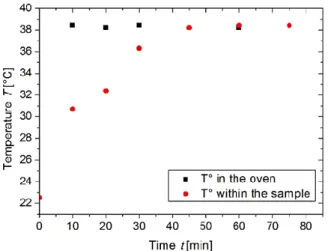
Using a microprocessor thermometer (HANNA instruments, HI 8757), we characterised the evolution of the temperature in the oven and at the center of the sphere template. As shown in the example of Figure 7, the fluctuations of the oven temperature are of the order of 0.5 °C and it takes about 60 min for the sphere packing to reach the temperature of the oven. In order to avoid misinterpretation of the data due to this initial equilibration time, we characterised the template morphology for samples which spent at least 2 hours in the oven.
Figure 4: a) Photograph of paraffin spheres taken under a microscope. b) Image thresholded with selected spheres in red. c) Same image after using the separation tool provided with the Keyence Software. The inset shows a zoom on the selected group of spheres. d) Probability density function (PDF) of the radii of the paraffin spheres and the corresponding Gaussian fits for two different rotation speeds. e-f) PDF of selected sphere ranges after sieving for different rotation speeds and sieve dimensions.
Figure 5: Calibration curve of the oven for a set temperature at 38 °C (black points) and in the centre of the sample (red points).
3.4) Generation of macro-porous polyurethane
All polyurethane precursors are kindly supplied by FoamPartner (Gontenschwil, Swiss). We use the polyether-based triol Voranol 6150 and the diisocyanate M220 (both from DOW chemical) at a weight ratio of 13.4 to 1 to ensure an isocyanate index of 100. The polyurethane is obtained by simply mixing both components (Ultra Turrax, IKA ®T25 at 20K rpm, for 2 minutes). No catalyst is added to let enough time for the liquid mixture to infiltrate the sphere packing before solidification and to maintain a low reaction temperature to avoid additional sphere deformation. The mixture is poured directly onto the sintered sphere packing where it spontaneously fills the interstitial spaces between the beads. This filling process takes about 1 h. The sample is then left at room temperature for 72 h to ensure full solidification of the polyurethane.
Finally, we use Soxhlet extraction by n-hexane for 6 h, at 100°C in order to remove the paraffin spheres. The resulting porous polyurethanes are let to dry overnight under a fume hood at room temperature.
3.5) Scanning electron microscopy (SEM)
We image the sphere templates and the porous polyurethanes with an SEM Hitachi SU8010 (FEG-SEM) under 1 KeV voltage acceleration to investigate the pore and interconnection morphologies. The samples are imaged directly without metallisation. Before observation of the paraffin sphere
templates, they are quenched in liquid nitrogen at -196 °C and
then directly broken. This helps to conserve the template structure and, in particular, the geometry of the necks. The PU
sponges are cut at room temperature using a cutter knife and
imaged directly (Figure 6a).
The obtained images are treated with ImageJ software. In the case of the sphere templates, the pore radius 𝑅 and interconnection radius 𝑟 were measured by hand, taking into account at least 130 pores and interconnections for each data point to ensure good statistic.
In the case of the PU sponges, the interconnection sizes are calculated semi-automatically by employing the « particle analysis » tool (Figure 6c) after proper thresholding (Figure 6b) of the initial image (Figure 6a). In order to exclude zones which are not interconnections, only objects with a circularity higher than 0.5 are selected. We also only considered “particles” whose area ranges between 60 and 6000 μm². Since the circular interconnections are imaged at different angles, they commonly appear as ellipses. We use the measurement of half of the major axis of the ellipse (Frenet diametre), which corresponds to the real radius 𝑟 of the interconnections. For each data point we measure at least 200 interconnections to ensure good statistics.
The average values of the sphere radii 𝑅 and the interconnection radii 𝑟 are obtained from the arithmetic mean of the distributions, while we use the standard deviation as the error of one sample.
The error bars given in the unscaled graphs of Section 4.2 are obtained by repeating each experiment three times. The error bar corresponds to the standard deviation calculated for the overall set of values.
The error bars in scaled graphs (such as Figure 11) are obtained by linear error propagation. If we plot the function 𝐹 = 𝑟/𝑅1−
its relative error is given by
∆𝐹 𝐹 = [ ∆𝑟 𝑟 + (1 − 𝛼) ∆𝑅 𝑅], (23)
3.6) DSC analysis
We place 8.2 mg of the paraffin in a stainless steel capsule and put the capsule inside the instrument (PerkinElmer DSC 8500). Experiments were done under nitrogen atmosphere which allow to ensure a chemically inert environment. Figure 7 shows the curves obtained by heating/cooling between 25 °C and 80°C with a ramp of 10 °C/min. A first cycle has also been performed to erase the thermal history of the paraffin (not shown here). The endothermic peak at 55-67°C corresponds to the melting point which is in accordance with the range given by the supplier.
Figure 7: DSC curve of the paraffin wax used for the sphere templating.
However, one can also see a slight shoulder in the curve around 40°C which indicates that some paraffin chains may have started to melt already before the melting point. All our experiments were typically conducted between 35 and 42°C, thus, even if our working temperatures were below the melting transition, due to the polydisperse nature of paraffin, we expected that some hydrocarbon chains may have melted at these temperatures.
3.7) Rheology of paraffin
Experiments were conducted with a rheometer MCR 702 MultiDrive® from Anton Paar at various temperatures (30, 32, 34, 36, 38, 40, 42 °C). The cone plate configuration with an angle of 5° was used. Before the tests, platelets of paraffin wax were deposited onto the peltier plate and heated up to 60 °C to transform the paraffin into its liquid state. The rheometre cone was then approached until having full contact with the wax and down to the desired gap size. The paraffin was then cooled down at 20 °C/min until 25 °C to form the solid sample between the plateaux. Afterwards, the solidified sample is heated at 5 °C/min to the desired temperature to simulate the conditions in the oven. The rheological measurements are started once the sample has reached thermal equilibrium. The dynamic viscosity of the paraffin was obtained with a frequency sweep from 0.01 up to 10 Hz (50 points log spaced) at a constant strain of 0,1 %. he resulting (𝜔) curves are shown in Figure 8. They are well fitted by a simple power law
𝜂(𝜔) = 𝜉(𝑇)𝜔𝜈(𝑇), (24) Figure 6: a) SEM image of a porous polyurethane sample. b) Thresholded image of (a) to bring out the interconnections. c) Objects with circularity above 0.5 are selected as interconnections. d) Probability Density Function (PDF) of the interconnection radii r corresponding to the image (a) and the corresponding Gaussian fit (red curve).
Figure 8: Frequency-dependent shear viscosity of paraffin for different temperatures obtained by oscillatory shear rheology. Dashed lines indicate the fit obtained using the power law of Equ.(24). The associated fit parameters are given in Table 1.
using 𝜉(𝑇) and 𝜈(𝑇) as temperature-dependent fit parameters with 𝜈 ∈ ]0,1[ . The obtained values are listed in Table 1. Table 1: Fit parameters obtained after fitting Equ. (24) to the viscosity data obtained from rheology.
Temperature T (°C) (Pas) 30 449 148 -0.66 34 272 835 -0.61 36 206 597 -0.59 38 158 684 -0.57 40 117 897 -0.56 42 93 655 -0.59
4) Results and discussion
4.1) General description
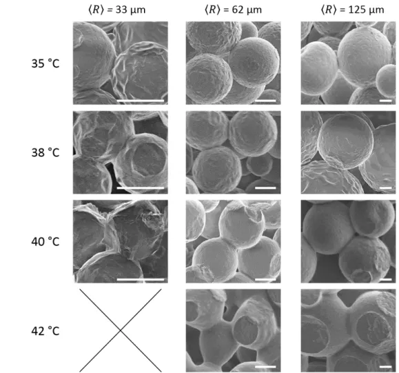
Figure 9 shows a series of SEM images obtained for different sphere sizes and sintering temperatures after 18 hours of sintering time. Images after shorter sintering times show the same overall pattern but with less pronounced evolutions of the interconnections. Following the indications of Figure 1, we denote in the following 𝑅 the average radius of the spheres and 𝑟 the average radius of their interconnections.
From Figure 9 we can see very clearly the influence of the sphere radius 𝑅 and the sintering temperature T on the kinetics of formation of the interconnections. Globally, one observes that the radius 𝑟 of the interconnections increases with temperature. For example, at the lowest temperature and for the largest sphere sizes, the interconnections are almost singularities as it is the case for two hard spheres in contact. With increasing temperature or decreasing sphere size, the deformation is accelerated and the spheres start to flatten
earlier, forming a neck which can be observed from the side or through the footprint left after breaking the contact (i.e. the flat circles visible on the spheres). This flattening is a consequence of the “crushing flow” (Figure 2a Section 2) as described by Milner. It is clearly seen at 40°C for the largest spheres (𝑅 = 125 µm). For smaller spheres at higher temperatures, one observes that the radius of curvature in the cusp of the interconnection increases, i.e. the interconnection does not only grow in area but its boundary also becomes increasingly rounded. This is a signature of the onset of the so-called “smoothing flow” shown Figure 2b and discussed Sections 2.2. For the smallest spheres (𝑅 = 33 µm), the spheres coalesce completely at the highest temperature. This is why the item is represented by a cross in Figure 9.
Figure 10 shows the macro-porous polyurethanes obtained from the sphere templates shown in Figure 9. One notices that these are accurate negative copies of the initial template, containing spherical pores with circular interconnections. Accordingly, the radii of the interconnections increase in the same manner with increasing temperature and decreasing sphere radius. For the structures with the smallest pore radii, the interstices between the spheres are too small to allow for the polymer to spread homogeneously through the template. This is why these structures are represented by a cross in Figure 10. One notices that when the radius of the interconnections becomes of the order of the sphere radius, the structure loses its spherical morphology and evolves into a very open “bicontinous like” shape, which may be interesting for applications looking to optimise permeability while maintaining a characteristic pore size and a certain mechanical stability of the material. This transition happens between 35 and 38°C for the smallest pore radius (𝑅 = 33 µm) and between 40 and 42°C for the structure with the intermediate pore radius (𝑅 = 62 µm). For the largest pore diameters, the transition happens above 42°C.
Figure 9: SEM images of paraffin sphere templates having an average radius of 〈𝑹〉 = 33 µm (left column), 〈𝑹〉= 62 µm (column in the middle) and 〈𝑹〉 = 125 µm (right column) for several sintering temperatures. All templates were sintered for 18 hours. The scale bars are 50 µm.
4.2) Quantitative analysis and interpretation
Figure 11a shows an example of the evolution of the mean radius 𝑟 of the interconnections with time for three sphere radii (𝑅 = 33, 62 and 125 m) at 38°C. The error bars are obtained by the procedure described in Section 3.5. Despite some scatter, all curves follow a clear trend: a rapid increase of 𝑟 over a few hours is followed by a much slower evolution. Moreover, the evolution of 𝑟 depends clearly on the radius 𝑅 of the spheres.
Figure 11b shows for the same sphere radii, how the mean radius 𝑟 of the interconnections after 18 h sintering time depends on the sintering temperature T in a temperature range of 35-42°C. As expected, 𝑟 increases significantly with the sintering temperature and the sphere radius 𝑅.
Figure 11c,d show the same data rescaled by the historic scaling of Frenkel, given in Equ. (3) with = ½ . Figure 11e,f exploit the new viscous scaling provided by Milner’s Newtonian model, given by Equ. (3) with = 1/3. A first observation is that both scalings collapse the data fairly well onto a mastercurve within the experimental scatter, implying that for the chosen data both
scalings capture reasonably well the main underlying mechanisms. It also confirms that the ratio ( /) evolves with temperature in the same manner for all sphere sizes, implying the absence of finite size effects. The interpretation of the overall shape of the master curves depends on how exactly ( /) depends on temperature, which is discussed in more
detail later.
For illustrative purposes, Figure 11 contains only a subset of the full data set. The full data set is shown in Figure 12a for different sphere sizes (R = 33, 62, 125 m), sintering temperatures (T = 35, 38, 40, 42°C) and sintering times (2, 4, 7, 11, 18 hours). To scale all data within the same plot and to allow comparison between the models, we rewrite Equ. (3) to obtain the scaling
[ 〈𝑟(𝑡)〉 𝑡𝛼〈𝑅〉1−𝛼]
1 𝛼⁄
= 𝐶𝛼𝛾𝜂= 𝑓𝛼(𝑇), (25)
where 𝑓𝛼(𝑇) is a function of the temperature T only. The
resulting mastercurve for Frenkel’s scaling is shown in Figure 12b (R2 = 0.48), while Milner’s scaling is shown in Figure 12c (R2
= 0.61). A first observation is that while the data remain fairly
scattered after application of Frenkel’s scaling, Milner’s scaling collapses the data somewhat more convincingly, especially for the lower temperatures. To quantify the quality of the scaling, we fit the scaled data to a second order polynomial
[ 〈𝑟(𝑡)〉 𝑡𝛼〈𝑅〉1−𝛼] 1 𝛼⁄ = 𝑎(𝑇 − 35°𝐶)2+ 𝑏(𝑇 − 35°𝐶) + 𝑐 ≡ 𝐵 𝛼(𝑇), (26)
with a,b and c being the fitting parameters. This captures in particular the temperature variation of the viscosity of the
paraffin, which is quite important since the experiments are done in the first endothermic shoulder in the DSC curve (Figure 7) close to the melting transition. The temperature variation of
can be assumed negligible in comparison to that of in our
temperature range. The resulting fits are shown by the red lines in Figure 12b and c, while the resulting fit parameters and coefficient of determination R2 are given in Table 2. Values of 𝛾
𝜂
for Frenkel’s and Milner’s viscous model can therefore be
approximated by using Equ. (26) and the associated fit parameters.
Table 2: Summary of exponents and fit parameters obtained for the different scaling by fitting Equ (26). Name a [µm.h-1.K-2] b [µm.h-1.K-1] c [µm.h-1] R 2 Frenkel’s scaling 1/2 0.05 0.01 0.76 0.48 Milner’s viscous scaling 1/3 0.03 -0.03 0.18 0.61
Figure 11 : Evolution of the average interconnection radius r as (a) a function of the sintering time t at 38°C and (b) as a function of sintering temperature T after 18 hfor three different sphere radii. (a,b) Unscaled results. (c,d) Results of a,b rescaled using Frenkel’s scaling (Equ. (3) with = ½). (e,f) Results of a,b rescaled using Milner’s Newtonian scaling (Equ. (3) with = 1/3). Error bars are calculated according to Section 3.5.
It is particularly evident by plotting the experimental results of 𝑟/𝑅 versus the theoretically predicted in Figure 13 Milner’s viscous scaling collapses slightly better the data than Frenkel’s scaling. Nevertheless, the spread in the collapsed data remains unsatisfyingly large, indicating the lack an important ingredient in either model. The origin of this scatter becomes readily evident by considering the rheology data of the paraffin shown in Figure 8. While the scalings used until now can take into account the dependence of the viscosity of the paraffin on
temperature, they cannot account for its dependence on the characteristic time scale of solicitation i.e. the strongly visco-elastic behaviour displayed by the paraffin in Figure 8 is not reflected in any of the models used up to this point.
We therefore use the visco-elastic model provided by Milner (Equ. (15) in Section 2.3) with the appropriate modification that takes into account the rheological response of our paraffin, given by Equ. (21). The only unknown (temperature-dependent) parameter is the surface tension 𝛾 of the paraffin, while 𝜈 and 𝜉 are known from fitting data of the rheological measurements (Figure 8). We therefore performed a fit to all data assuming for
(𝑇) a second order polynomial expansion around the lowest temperature 35°C: 𝛾(𝑇) = (𝛾0+ (𝑇𝑗− 35)𝛾1+ (𝑇𝑗− 35)
2
𝛾2)
For this purpose, we performed a fit with the function “fminsearch” of Matlab© which looks for a minimum for
𝐹(𝑎0, 𝑎1, 𝑎2) = ∑ [〈𝑟𝑗〉 − 𝐶𝑗 1 3𝑡 𝑗 (1−𝜈𝑗) 3 〈𝑅 𝑗〉 2 3(𝛾0+ (𝑇𝑗− 35)𝛾1+ (𝑇𝑗− 𝑗 35)2𝛾2) 1 3] 2 , (27) where 𝐶𝑗≡ 3𝜋 sin (𝜋𝜈2 )𝑗 32𝜉𝑗(1 − 𝜈𝑗)𝛤(1 − 𝜈𝑗). (28)
Here 𝑗 represents a measure, namely a set of time 𝑡𝑗 or
temperature 𝑇𝑗 (determining the viscoelastic parameters 𝜉𝑗=
𝜉(𝑇𝑗)and 𝜈𝑗= 𝜈(𝑇𝑗), average radii of the spheres 〈𝑅𝑗〉 and the
corresponding average radii of the interconnections 〈𝑟𝑗〉).
Figure 14 plots the obtained fit for 𝛾(𝑇) together with the surface tension values obtained for each data point using the reshuffled expression of Equ. (21): 𝛾(𝑇𝑗) = {𝑟𝑗/
[𝐶𝑗1/3𝑡𝑗(1−𝜈𝑗)/3𝑅
𝑗2/3]}. The characteristic values of 𝛾 0.01 N/m
are very satisfactory, since they are compatible with the values for the surface tension of paraffin measured in the literature (see
www.accudynet.com/polymer_surface_data/paraffin.pdf), where it is found that 𝛾 ≈ 0.02 N/m. Nevertheless, the
Figure 12: a) Summary of all data without any scaling. (b) Frenkel’s scaling (α = ½) (c) Milner’s scaling (α = 1/3). The red lines are the best fits obtained using Equ.(26). The resulting fitting parameters are summarised in Table 2.
temperature dependence of 𝛾(𝑇) we found is not physical, since 𝛾(𝑇) has to be a decreasing function of temperature. However, a significant increase in temperature is observed only for the highest temperature T= 42 °C. For the lower temperatures, 𝛾 is essentially independent of temperature. At the highest temperature, the problem may presumably arise from a failure of our assumption according to which the
viscoelastic behaviour of 𝜂(𝜔) = 𝜉𝜔−𝜈could be extended to the extremely low frequency range appropriated for our experiment. At this temperature, the longest relaxation time of the paraffin may be shorter than the 18 hours of our longest experiment. Another possible cause of discrepancy could be sought in the fact that for the highest temperature, the sintering dynamics is the fastest, and therefore, the largest values of 𝑟/𝑅 are measured. As a result, some quantitative discrepancies with the theory which is intended to describe the
Figure 13: Experimental values of 𝑟(𝑡)/𝑅 as a function of the values predicted by the different theories, the best fit of the unknown parameter have been chosen. Data which is perfectly described by the theory would fall onto the black line X=Y
𝑟 /𝑅 << 1 regime only, might show up here. In particular, the smoothing flow described in Section 2.2 may be no longer negligible here.
Using the obtained expression for (𝑇), we plot in Figure 13 the experimental values of 〈𝑟(𝑡)〉/〈𝑅〉 versus the values predicted by Milner’s visco-elastic scaling given by Equ. (21). This comparison shows convincingly that Milner’s visco-elastic model captures very well the experimental data in collapsing it fairly neatly on the line X = Y. For 〈𝑟(𝑡)〉/〈𝑅〉 > 0.25 the
Figure 14: Best fit results for the surface tension (T) with all the data available. The
different sizes are represented by circles (〈𝑹〉= 33 µm), squares (〈𝑹〉= 62 µm), and diamonds (〈𝑹〉= 125 µm) respectively. The different times: t = 2, 4, 7, 11, 18 hours are represented by the colour marine blue, red, yellow, purple, green, and cyan, respectively.
experimental data is slightly above the theoretically predicted values. This deviation may be explained by three arguments. On the one hand it is coherent with the onset of the smoothing flow, which is expected to start playing a role for 𝑟/𝑅 > 0.25 and which follows a different scaling, as discussed in Section 2.2. The smoothing flow would lead to larger 〈𝑟(𝑡)〉/〈𝑅〉-values, as observed. On the other hand, our extrapolation of the power laws describing the rheology data (Section 3.7) may break down in this limit which concerns either high temperatures or long time scales. Besides, it is worth to mention that when neck radii approach the order of magnitude of sphere radii, cross interactions of close necks may not be negligible anymore and thus, account for the gap between experimental and theoretical values (see Figure 10). And last but not least, at these large 〈𝑟(𝑡)〉/〈𝑅〉 values, interconnections start to interact on the surfaces of the spheres, leading to a shift away from the scalings which are derived for isolated interconnections.
In summary we can state that both of Milner’s scalings capture our experiments better than Frenkel’s scaling, while the quality of the visco-elastic scaling clearly indicates the importance of
taking into account the Non-Newtonian nature of the paraffin spheres.
Conclusions
In this article we present the results of thoroughly conducted sintering experiments with paraffin spheres. All experimental results are compared to the historic scaling proposed by Frenkel and to the recent models proposed by S. Milner46,47. While both
models are similar in their approach, we believe that Milner’s approximation of the flow field being confined to the contact zone (Section 2.1) is physically better justified. The resulting
viscous model (Equ. (8)) leads to slightly different exponents
(1/3 instead of 1/2) and pre-factors (3/32 instead of 4) with respect to Frenkel’s model, with Milner’s model fitting slightly better our experimental data. However, a real breakthrough in the quality of the description of the data is made using Milner’s
visco-elastic model (Equ. (15)), which takes into account the
visco-elastic nature of the paraffin spheres. The general applicability of this model will allow a direct transfer of the predictions to other sphere systems, provided their visco-elastic properties can be quantified.
Milner’s visco-elastic model captures very well our data up to deformations of 〈𝑟(𝑡)〉/〈𝑅〉 0.25. Beyond this point, the onset of the smoothing flow (Section 2.2), interactions between contact areas or the breakdown of our rheological approximations may play a role.
In order to fully validate Milner’s model and its limits, it will be important to conduct future experiments with different types of model-spheres in which both, visco-elasticity and surface energy are known and controlled in a quantitative manner. It would be important to validate not only the Non-Newtonian model, but also to access the transition to the regime in which the smoothing flow becomes dominant. Last but not least, it would be interesting to analyse the influence of the multiple contacts on each sphere54.
Beyond the analysis of the sintering process, we successfully used the obtained sphere templates to generate macro-porous polyurethanes whose morphology can be finely tuned in a predictive manner thanks to Milner’s model. Since paraffin and polyurethane can be replaced by a wide range of alternative formulations, this approach can be transferred easily to a multitude of systems which require a fine control over the pore morphology. Indeed, by the knowledge of only a few parameters: surface tension, sphere size and the temperature-dependent rheological data (𝜈 and 𝜉), the sintering behaviour of the system can be predicted
Conflicts of interest
Acknowledgements
This work has been published within the IdEx Unistra framework (Chaire W. Drenckhan) and has, as such, benefited from funding from the state, managed by the French National Research Agency as part of the 'Investments for the future' program. The work was also supported by the Institut Carnot MICA (project DiaArt) and by an ERC Consolidator Grant (agreement 819511 – METAFOAM).
We thank Scot Milner for having shared his detailed, originally unpublished analysis on which much of our analytical work is based and for various email exchanges on the matter. We thank the platforms “Characterisation” (Mélanie Legros and Catherine Saettel) and “Microscopy” (Marc Schmutz and Alain Carvalho) for access to project-relevant devices and for discussion. We thank Robin Bollache and Damien Favier for help with the experiments. We thank Fouzia Boulmedais, Alexandre Collard and Jörg Baschnagel and for scientific discussions. We also acknowledge the first tomographic analysis of our samples by Matthias Schröter and Gaetan Dalongeville. Last but not least, we thank FOAMPARTNER for advice and for providing the chemicals required for the PU synthesis.
Notes and references
1 U. Betke and A. Lieb, Adv. Eng. Mater., 2018, 20, 1800252. 2 A. G. Evans, J. W. Hutchinson and M. F. Ashby, Prog. Mater.
Sci., 1998, 43, 171–221.
3 M. Inagaki, J. Qiu and Q. Guo, Carbon N. Y., 2015, 87, 128–152. 4 L. Glicksman, M. Schuetz and M. Sinofsky, Int. J. Heat Mass
Transf., 1987, 30, 187–197.
5 S. C. Isabelle Cantat, Sylvie Cohen-Addad, Florence Elias, Francois Graner, Reinhard Hohler, Olivier Pitois, Florence Rouyer, Arnaud Saint-Jalmes, Ruth Flatman, Foams: Structure and
Dynamics, Oxford University Press, 2013.
6 H. Janik and M. Marzec, Mater. Sci. Eng. C, 2015, 48, 586–591. 7 E. C. Hammel, O. L.-R. Ighodaro and O. I. Okoli, Ceram. Int., 2014, 40, 15351–15370.
8 M. A. H. Michael S. Silverstein, Neil R. Cameron, Porous
Polymers, Wiley, 2011.
9 J. Banhart, Prog. Mater. Sci., 2001, 46, 559–632.
10 V. H. Trinh, V. Langlois, J. Guilleminot, C. Perrot, Y. Khidas and O. Pitois, Mater. Des., 2019, 162, 345–361.
11 D. Jahani, A. Ameli, P. U. Jung, M. R. Barzegari, C. B. Park and H. Naguib, Mater. Des., 2014, 53, 20–28.
12 J. . Richardson, Y. Peng and D. Remue, Appl. Catal. A Gen., 2000, 204, 19–32.
13 V. Langlois, V. H. Trinh, C. Lusso, C. Perrot, X. Chateau, Y. Khidas and O. Pitois, Phys. Rev. E, 2018, 97, 53111.
14 G. Lutzweiler, J. Barthès, G. Koenig, H. Kerdjoudj, J. Mayingi, F. Boulmedais, P. Schaaf, W. Drenckhan and N. E. Vrana, ACS Appl.
Mater. Interfaces.
15 M. Costantini, C. Colosi, P. Mozetic, J. Jaroszewicz, A. Tosato, A. Rainer, M. Trombetta, Ś. Wojciech, M. Dentini and A. Barbetta, 2016, 62, 668–677.
16 L. R. Madden, D. J. Mortisen, E. M. Sussman, S. K. Dupras, J. A. Fugate, J. L. Cuy, K. D. Hauch, M. A. Laflamme, C. E. Murry and B. D. Ratner, Proc. Natl. Acad. Sci. U. S. A., 2010, 107, 15211–6. 17 S. W. Choi, Y. Zhang, M. R. Macewan and Y. Xia, Adv. Healthc.
Mater., 2013, 2, 145–154.
18 E. R. I. C. M. S. Ussman, M. I. C. H. Alpin, J. E. M. Uster, R. A. T. M. Oon and B. U. D. R. Atner, 2014, 42, 1508–1516.
19 S. Andrieux, W. Drenckhan and C. Stubenrauch, Langmuir, 2018, 34, 1581–1590.
Angew. Chemie, 2018, 130, 10176–10186.
21 M. S. Silverstein, Prog. Polym. Sci., 2014, 39, 199–234. 22 S. D. Kimmins and N. R. Cameron, Adv. Funct. Mater., 2011,
21, 211–225.
23 W. Drenckhan and A. Saint-Jalmes, Adv. Colloid Interface Sci., 2015, 222, 228–259.
24 H. Kim, S. Lee, Y. Han and J. Park, Mater. Chem. Phys., 2009,
113, 441–444.
25 A. Testouri, M. Ranft, C. Honorez, N. Kaabeche, J. Ferbitz, D. Freidank and W. Drenckhan, Adv. Eng. Mater., 2013, 15, 1086– 1098.
26 M. Costantini, C. Colosi, J. Guzowski, A. Barbetta, J. Jaroszewicz, W. Święszkowski, M. Dentini and P. Garstecki, J.
Mater. Chem. B, 2014, 2, 2290.
27 K. Yasunaga, R. A. Neff, X. D. Zhang and C. W. Macosko, J. Cell.
Plast., 1996, 32, 427–448.
28 D. Tammaro, G. D’Avino, E. Di Maio, R. Pasquino, M. M. Villone, D. Gonzales, M. Groombridge, N. Grizzuti and P. L. Maffettone, Chem. Eng. J., 2016, 287, 492–502.
29 A. Stein, Microporous Mesoporous Mater., 2001, 44–45, 227– 239.
30 P. X. Ma and J.-W. Choi, Tissue Eng., 2001, 7, 23–33.
31 A. J. Marshall and B. D. Ratner, AIChE J., 2005, 51, 1221–1232. 32 S.-J. L. K. K, SINTERING, densification, grain growth &
microstructure, 2005.
33 S. I. Somo, B. Akar, E. S. Bayrak, J. C. Larson, A. A. Appel, H. Mehdizadeh, A. Cinar and E. M. Brey, Tissue Eng. Part C Methods, 2015, 21, 773–85.
34 R. Chen, H. Ma, L. Zhang and J. D. Bryers, Biotechnol. Bioeng., 2018, 115, 1086–1095.
35 V. J. Chen and P. X. Ma, Biomaterials, 2004, 25, 2065–2073. 36 J. Zhang, H. Zhang, L. Wu and J. Ding, J. Mater. Sci., 2006, 41, 1725–1731.
37 S. Grenier, M. Sandig and K. Mequanint, J. Biomed. Mater.
Res. A, 2007, 82, 802–9.
38 K. Takagi, T. Takahashi, K. Kikuchi and A. Kawasaki, J. Eur.
Ceram. Soc., 2010, 30, 2049–2055.
39 K. Zhao, Y. F. Tang, Y. S. Qin and D. F. Luo, J. Eur. Ceram. Soc., 2011, 31, 225–229.
40 M. Descamps, T. Duhoo, F. Monchau, J. Lu, P. Hardouin, J. C. Hornez and A. Leriche, J. Eur. Ceram. Soc., 2008, 28, 149–157. 41 FRENKEL and J. J., J. Phys., 1945, 9, 385.
42 L. Verbelen, S. Dadbakhsh, M. Van den Eynde, J.-P. Kruth, B. Goderis and P. Van Puyvelde, Eur. Polym. J., 2016, 75, 163–174. 43 O. Pokluda, C. T. Bellehumeur and J. Vlachopoulos, AIChE J., 1997, 43, 3253–3256.
44 C. T. Bellehumeur, M. Kontopoulou and J. Vlachopoulos,
Rheol. Acta, 1998, 37, 270–278.
45 S. Mazur, R. Beckerbauer and J. Buckholz, Langmuir, 1997, 13, 4287–4294.
46 S. T. Milner, .
47 L. M. Ramírez, S. T. Milner, C. E. Snyder, R. H. Colby and D. Velegol, Langmuir, 2010, 26, 7644–7649.
48 S. Himran, A. Suwono and G. A. Mansoori, Energy Sources, 1994, 16, 117–128.
49 E. M. L. L. D. Landau, Fluid Mechanics, Elsevier, 2nd edn., 1987.
50 D. A. Spence, J. Elast., 1975, 5, 297–319. 51 M. Rubinstein, Polymer Physics, 2003.
52 S. Mazur and D. J. Plazek, Prog. Org. coatings, 1994, 24, 225– 236.
53 I. S. Gradshteyn and I. M. Ryzhik, Table of integrals, series, and
products, Academic press, 2014.
54 G. Ginot, R. Höhler, S. Mariot, A. Kraynik and W. Drenckhan,