COSMOLOGICAL CONSTRAINTS FROM GALAXY CLUSTERS
IN THE 2500 SQUARE-DEGREE SPT-SZ SURVEY
The MIT Faculty has made this article openly available.
Please share
how this access benefits you. Your story matters.
Citation
Haan, T. de; Benson, B. A.; Bleem, L. E.; Allen, S. W.; Applegate, D.
E.; Ashby, M. L. N.; Bautz, M. et al. “COSMOLOGICAL CONSTRAINTS
FROM GALAXY CLUSTERS IN THE 2500 SQUARE-DEGREE SPT-SZ
SURVEY.” The Astrophysical Journal 832, no. 1 (November 2016): 95
© 2016 The American Astronomical Society
As Published
http://dx.doi.org/10.3847/0004-637x/832/1/95
Publisher
IOP Publishing
Version
Final published version
Citable link
http://hdl.handle.net/1721.1/109811
Terms of Use
Article is made available in accordance with the publisher's
policy and may be subject to US copyright law. Please refer to the
publisher's site for terms of use.
COSMOLOGICAL CONSTRAINTS FROM GALAXY CLUSTERS IN THE 2500 SQUARE-DEGREE SPT-SZ
SURVEY
T. de Haan1,2, B. A. Benson3,4,5, L. E. Bleem4,6,7, S. W. Allen8,9,10, D. E. Applegate11, M. L. N. Ashby12, M. Bautz13, M. Bayliss12,14, S. Bocquet4,7,15,16, M. Brodwin17, J. E. Carlstrom3,4,6,7,18, C. L. Chang3,4,7, I. Chiu15,16, H-M. Cho19,
A. Clocchiatti20, T. M. Crawford3,4, A. T. Crites3,4,21, S. Desai15,16, J. P. Dietrich15,16, M. A. Dobbs2,22, A. N. Doucouliagos23, R. J. Foley24,25, W. R. Forman12, G. P. Garmire26, E. M. George1,27, M. D. Gladders3,4, A. H. Gonzalez28, N. Gupta15,16, N. W. Halverson29, J. Hlavacek-Larrondo9,30,31, H. Hoekstra32, G. P. Holder2,
W. L. Holzapfel1, Z. Hou4,6, J. D. Hrubes33, N. Huang1, C. Jones12, R. Keisler4,6,8,9, L. Knox34, A. T. Lee1,35, E. M. Leitch3,4, A. von der Linden8,9,36,37, D. Luong-Van33, A. Mantz4,8,9, D. P. Marrone38, M. McDonald13, J. J. McMahon39, S. S. Meyer3,4,6,18, L. M. Mocanu3,4, J. J. Mohr15,16,27, S. S. Murray12, S. Padin3,4,21, C. Pryke40, D. Rapetti15,16, C. L. Reichardt23, A. Rest41, J. Ruel14, J. E. Ruhl42, B. R. Saliwanchik42, A. Saro15,16, J. T. Sayre29, K. K. Schaffer4,18,43, T. Schrabback11, E. Shirokoff3,4, J. Song39,44, H. G. Spieler35, B. Stalder12, S. A. Stanford34,45, Z. Staniszewski42, A. A. Stark12, K. T. Story8,9, C. W. Stubbs12,14, K. Vanderlinde46,47, J. D. Vieira24,25, A. Vikhlinin12,
R. Williamson3,4,21, and A. Zenteno48
1
Department of Physics, University of California, Berkeley, CA 94720, USA 2Department of Physics,McGill University, Montreal, Quebec H3A 2T8, Canada 3
Department of Astronomy and Astrophysics, University of Chicago, Chicago, IL 60637, USA 4
Kavli Institute for Cosmological Physics, University of Chicago, Chicago, IL 60637, USA 5
Fermi National Accelerator Laboratory, Batavia, IL 60510-0500, USA 6
Department of Physics, University of Chicago, Chicago, IL 60637, USA 7
Argonne National Laboratory, Argonne, IL 60439, USA 8
Kavli Institute for Particle Astrophysics and Cosmology, Stanford University, 452 Lomita Mall, Stanford, CA 94305, USA 9
Department of Physics, Stanford University, 382 Via Pueblo Mall, Stanford, CA 94305, USA 10
SLAC National Accelerator Laboratory, 2575 Sand Hill Road, Menlo Park, CA 94025, USA 11Argelander-Institut für Astronomie, Auf dem Hügel 71, D-53121 Bonn, Germany
12
Harvard-Smithsonian Center for Astrophysics, Cambridge, MA 02138, USA 13
Kavli Institute for Astrophysics and Space Research, Massachusetts Institute of Technology, 77 Massachusetts Avenue, Cambridge, MA 02139, USA 14
Department of Physics, Harvard University, 17 Oxford Street, Cambridge, MA 02138, USA 15
Faculty of Physics, Ludwig-Maximilians-Universität, Scheinerstr. 1, D-81679 Munich, Germany 16
Excellence Cluster universe, Boltzmannstr. 2, D-85748 Garching, Germany 17
Department of Physics and Astronomy, University of Missouri, 5110 Rockhill Road, Kansas City, MO 64110, USA 18
Enrico Fermi Institute, University of Chicago, Chicago, IL 60637, USA 19
NIST Quantum Devices Group, Boulder, CO 80305, USA
20Departamento de Astronomia y Astrosifica, Pontificia Universidad Catolica, Chile 21
California Institute of Technology, Pasadena, CA 91125, USA
22Canadian Institute for Advanced Research, CIFAR Program in Cosmology and Gravity, Toronto, ON, M5G 1Z8, Canada 23
School of Physics, University of Melbourne, Parkville, VIC 3010, Australia 24
Astronomy Department, University of Illinois at Urbana-Champaign, 1002 W. Green Street, Urbana, IL 61801, USA 25
Department of Physics, University of Illinois Urbana-Champaign, 1110 W. Green Street, Urbana, IL 61801, USA 26
Huntingdon Institute for X-ray Astronomy, LLC, Huntingdon, PA 16652, USA 27
Max Planck Institute for Extraterrestrial Physics, Giessenbachstr. 1, D-85748 Garching, Germany 28
Department of Astronomy, University of Florida, Gainesville, FL 32611, USA 29
Department of Astrophysical and Planetary Sciences and Department of Physics, University of Colorado, Boulder, CO 80309, USA 30
Department of Physics, Université de Montréal, Montrea, Quebec H3T 1J4, Canada 31
Kavli Institute for Particle Astrophysics and Cosmology, Stanford University, 452 Lomita Mall, Stanford, CA 94305-4085, USA 32
Leiden Observatory, Leiden University, Niels Bohrweg 2, 2333 CA, Leiden, The Netherlands 33
University of Chicago, Chicago, IL 60637, USA 34
Department of Physics, University of California, Davis, CA 95616, USA 35
Physics Division, Lawrence Berkeley National Laboratory, Berkeley, CA 94720, USA 36
Department of Physics and Astronomy, Stony Brook University, Stony Brook, NY 11794, USA 37
Dark Cosmology Centre, Niels Bohr Institute, University of Copenhagen Juliane Maries Vej 30, DK-2100 Copenhagen, Denmark 38
Steward Observatory, University of Arizona, 933 North Cherry Avenue, Tucson, AZ 85721, USA 39
Department of Physics, University of Michigan, Ann Arbor, MI 48109, USA 40
Department of Physics, University of Minnesota, Minneapolis, MN 55455, USA 41
Space Telescope Science Institute, 3700 San Martin Dr., Baltimore, MD 21218, USA 42
Physics Department, Center for Education and Research in Cosmology and Astrophysics, Case Western Reserve University, Cleveland, OH 44106, USA 43
Liberal Arts Department, School of the Art Institute of Chicago, Chicago, IL 60603, USA 44
Korea Astronomy and Space Science Institute, Daejeon 305-348, Korea 45
Institute of Geophysics and Planetary Physics, Lawrence Livermore National Laboratory, Livermore, CA 94551, USA 46
Dunlap Institute for Astronomy & Astrophysics, University of Toronto, 50 St George St, Toronto, ON, M5S 3H4, Canada 47
Department of Astronomy & Astrophysics, University of Toronto, 50 St George St, Toronto, ON, M5S 3H4, Canada 48
Cerro Tololo Inter-American Observatory, Casilla 603, La Serena, Chile
Received 2016 March 21; revised 2016 August 15; accepted 2016 September 7; published 2016 November 18
ABSTRACT
We present cosmological parameter constraints obtained from galaxy clusters identified by their Sunyaev– Zel’dovich effect signature in the 2500 square-degree South Pole Telescope Sunyaev Zel’dovich (SPT-SZ) survey.
We consider the 377 cluster candidates identified at >z 0.25 with a detection significance greater than five,
corresponding to the 95% purity threshold for the survey. We compute constraints on cosmological models using the measured cluster abundance as a function of mass and redshift. We include additional constraints from multi-wavelength observations, including Chandra X-ray data for 82 clusters and a weak lensing-based prior on the normalization of the mass-observable scaling relations. Assuming a spatiallyflat ΛCDM cosmology, we combine the cluster data with a prior on H0and find s =8 0.7840.039and W =m 0.2890.042, with the parameter
combination s W8( m 0.27)0.3=0.7970.031. These results are in good agreement with constraints from the cosmic microwave background (CMB) from SPT, WMAP, and Planck, as well as with constraints from other cluster data sets. We also consider several extensions toΛCDM, including models in which the equation of state of dark energy w, the species-summed neutrino mass, and/or the effective number of relativistic species (Neff) are free
parameters. When combined with constraints from the Planck CMB, H0, baryon acoustic oscillation, and SNe,
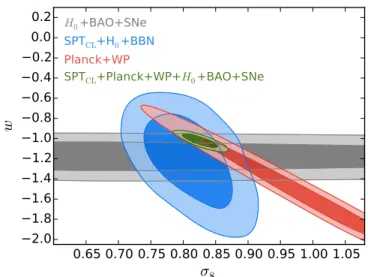
adding the SPT cluster data improves the w constraint by 14%, tow= -1.0230.042. Key words: cosmology: observations – galaxies: clusters: general
1. INTRODUCTION
Galaxy clusters trace extreme peaks in the matter density field on megaparsec scales. The abundance of these peaks as a function of mass and redshift is highly sensitive to the matter density and the growth of structure(e.g., Allen et al.2011). As
this abundance can be predicted with sufficient accuracy for a given cosmology (Holder & Carlstrom 2001; Tinker et al. 2008; Bhattacharya et al.2011), even modest
measure-ments of cluster abundance can yield powerful cosmological constraints. These constraints are particularly powerful when combined with or compared to independent constraints from probes such as the power spectrum of the cosmic microwave background (CMB) and baryon acoustic oscillations (BAOs). Taken together, growth-based and geometrical probes can place significantly tighter constraints on parameters such as the equation of state of dark energy than either one independently, because of nearly orthogonal parameter degeneracies. Con-sidered independently, these constraints provide a consistency test of the dark energy paradigm and the validity of general relativity (Ishak et al. 2006; Mortonson et al. 2009, 2010; Rapetti et al. 2009, 2010; Zhan et al. 2009; Acquaviva & Gawiser 2010; Vanderveld et al.2012).
In recent years, constraints on cosmological parameters from cluster abundance measurements have advanced significantly using cluster samples selected at X-ray (e.g., Vikhlinin et al. 2009b; Mantz et al. 2010, 2015), optical (e.g., Rozo
et al. 2010), and millimeter (e.g., Hasselfield et al. 2013; Reichardt et al. 2013; Planck Collaboration et al. 2014b; Bocquet et al. 2015; Planck Collaboration et al. 2015)
wavelengths. The predominant millimeter-wave (mm-wave) signal from clusters arises from the thermal Sunyaev– Zel’dovich (tSZ) effect (Sunyaev & Zel’dovich 1972), i.e.,
the scattering of CMB photons by hot electrons in the intra-cluster medium(ICM). The surface brightness of the tSZ effect is redshift-independent, allowing high-resolution mm-wave surveys to obtain nearly mass-limited samples of clusters to arbitrarily high redshift. The ability to cleanly select clusters out to the redshift at which dark energy begins to contribute significantly to the energy budget of the universe ( ~z 1) is
particularly important for constraints on the dark energy equation of state and tests of the dark energy paradigm. Cluster surveys using high-resolution tSZ data are uniquely positioned to deliver such constraints(Carlstrom et al.2002).
The primary limitation to cosmological constraints from current cluster surveys at all wavelengths is an imperfect understanding of the relationship between the quantity that can be predicted from theory or simulations(the cluster mass or the
height of the associated density peak) and the observable property of the cluster that is used as a proxy for this quantity. The mass proxy can be the observable quantity used to construct the sample; it can also include observables from follow-up observations, often at different wavelengths than the cluster selection observable. Since the cluster abundance is an extremely steep function of mass, misestimation of the relation between the mass proxy and the true cluster mass can lead to significant biases on the resulting cosmological parameter constraints.
Different cluster mass proxies have distinct advantages and disadvantages related to the accuracy and precision with which they trace the true cluster mass and the expense of obtaining the data required to construct them. In terms of ultimate accuracy, or absence of bias, the current gold standard mass proxy is derived from measurements of weak gravitational lensing of background galaxies by clusters (see von der Linden et al. 2014b for a discussion). Optical mass measurements from weak gravitational lensing are observationally expensive to obtain at high redshift, and the scatter on individual cluster mass estimates is large. Gravitational lensing of the CMB by clusters is a promising future avenue for mass estimation(e.g., Baxter et al. 2015; Madhavacheril et al. 2015; Planck Collaboration et al. 2015). Cluster velocity dispersions, generally obtained through spectroscopic observations of tens of cluster member galaxies, are also mostly unaffected by complex ICM physics but are expensive observationally and have large scatter (e.g., Evrard et al. 2008; Saro et al. 2013; Sifón et al. 2013; Ruel et al. 2014), as well as uncertain
velocity bias (e.g., Munari et al.2013). Where weak lensing
(WL) measurements provide high accuracy, measurements of the gas mass Mgas, and/or of the integrated cluster pressure Y
provide high precision. Estimated from tSZ or X-ray data, integrated cluster pressure is predicted and measured to track cluster mass with low scatter(e.g., Motl et al.2005; Kravtsov et al. 2006; Nagai et al. 2007; Stanek et al. 2010), but its
relation to true cluster mass can be complicated by non-thermal pressure support in clusters (e.g., Evrard et al. 1996; Nagai et al.2007; Yu et al. 2015). Furthermore, robust Y estimates
require either relatively high-quality X-ray data (to provide deprojected temperature and density profiles), or tSZ measure-ments with accurate information on all cluster scales (sub-arcminute scales to the virial radius). Mass proxies built from the same data used to select clusters, such as optical richness, X-ray luminosity, and tSZ detection significance, come at no extra cost but can demonstrate high scatter and require external calibration data to tie them robustly to the true cluster mass.
In this work, we use a sample of clusters derived from the SPT-SZ survey, a three-band mm-wave survey of 2500 deg2of
the southern sky conducted with the South Pole Telescope (SPT, Carlstrom et al. 2011). The cluster selection method,
redshift determination, and sample characteristics are described in detail in Bleem et al.(2015, hereafterB15). We use the
mm-wave and redshift information from B15 in conjunction with targeted X-ray follow-up observations from Chandra to obtain cosmological constraints. The mass proxy we use is the tSZ detection significance ξ, calibrated using X-ray integrated pressure YX, which is in turn tied to true cluster mass using
optical WL measurements.
The paper is organized as follows. In Section2, we briefly describe the cluster sample, including the mm-wave data and analysis methods that went into producing the sample. We summarize the optical/infrared data and redshift estimation in Section 3, and the X-ray data and analysis methods in Section 4. The cosmological analysis methods are described in Section 5, and we present the cosmological parameter constraints in Section 6. We compare the cosmological constraints from this work to those from other cluster surveys in Section7, and we conclude in Section8.
When parameter constraints are reported, the best-fit value and uncertainties correspond to the mean and standard deviation of the posterior distribution. Cluster masses, denoted withM , refer to spherical overdensities for which the enclosedD
density is equal toΔ times the critical density, rc. Similarly,rD
refers to the associated radius such that MD= prDDrc z 4
3 3
( ). 2. SZ DATA AND METHODS
The cluster sample used in this work is a subset of that previously presented inB15. We choose clusters with redshift
>
z 0.25 and detection significance x > 5. The significance cut
was chosen such that the resulting catalog has high (~95%) purity, and the redshift cut allows for a nearly redshift-independent selection function (Vanderlinde et al. 2010, hereafter V10). Our strategy for tying the cluster abundance
measurement to the cosmologically predicted halo mass function is to calibrate the SZ–mass scaling relation using Chandra X-ray measurements. The X-ray scaling relation is taken from Vikhlinin et al. (2009a, 2009b, hereafter V09), though we modify the overall normalization of this relation in Section 4.2 to be consistent with more recent WL measure-ments from Hoekstra et al. (2015, hereafter H15) and the
Weighing the Giants(WtG) project (Applegate et al.2014; von der Linden et al.2014a; Mantz et al.2015).
2.1. Sample of SZ Cluster Candidates
The SPT is a 10 m telescope located at the geographic South Pole. With a 1degree field of view and ∼1arcmin resolution, it was designed to rapidly map large areas of sky while being well matched to the angular size of high-redshift clusters. The SPT-SZ camera operated from 2007 through 2011 and consisted of a 960-element, photon-noise-limited bolometer array observing in three frequency bands centered at 95, 150, and 220GHz, though this work uses only the first two bands. The observation strategy and analysis for the 2500 square-degree SPT-SZ survey are described in many previous SPT papers(e.g., Schaffer et al.2011), and the analysis specific to
obtaining the cluster sample is described in B15. Briefly, the majority of the 2500 square-degree survey was performed
using the following scan strategy. The telescope is moved using a right-going scan in azimuth, followed by a left-going scan, followed by a step in elevation. This pattern is repeated until a 100 square degree patch of sky is observed. One such iteration is termed an observation, whereas the patch of sky is termed afield. In the only exception to this observing strategy, for two thirds of the data taken on onefield (ra21hdec-50), the scan pattern instead consisted of scans in elevation at a series of fixed azimuth positions. Each field was observed until a depth of m18 K-arcmin at 150GHz was reached. Table 1lists the 19fields that comprise the full survey. For more information on the properties of thefields, see Table 1 ofB15.
Two-dimensional maps of the sky are made by binning the time-ordered data(TOD), to which mild time-domain filtering has been applied, into 0.25 arcmin pixels. This produces estimates of the 95 and 150GHz sky, to which we apply a simultaneous spatial-spectral filter, yielding a filtered estimate of the tSZ sky, optimized for extracting cluster candidates. The candidates are identified using a peak-finding algorithm.
Due to the exact choice offield extent, as well as the finite footprint of the SPT-SZ array on the sky, the fields overlap slightly. The overlap regions only comprise ~2% of the total survey area, and for simplicity we choose to treat thefields as fully independent. As a result of this treatment, we would expect to double-count roughly 2% of cluster candidates, or seven to eight of our total number of candidates. In fact wefind nine cases of candidates with a very high probability of having been detected in two different fields (i.e., 18 total candidates that correspond to nine physical clusters). There is no bias to our cosmological constraints from this treatment. Our uncer-tainties will be very slightly underestimated, but this has a negligible effect on ourfinal cosmological constraints.
Table 1
The 19 SPT-SZ Fields with the Simulation-derived Inputs to the Cosmological Analysis of the 2500Square-degree Survey
Name afield bfield gfield
RA5H30DEC-55 16.79 4.60 1.33 RA23H30DEC-55 17.58 4.03 1.39 RA21HDEC-60 25.64 4.07 1.29 RA3H30DEC-60 20.53 4.70 1.25 RA21HDEC-50 25.28 4.14 1.11 RA4H10DEC-50 16.75 5.48 1.27 RA0H50DEC-50 20.76 5.11 1.14 RA2H30DEC-50 14.98 4.78 1.19 RA1HDEC-60 17.25 5.38 1.18 RA5H30DEC-45 15.91 4.81 1.08 RA6H30DEC-55 17.77 4.58 1.16 RA3H30DEC-42.5 16.85 4.31 1.20 RA23HDEC-62.5 14.90 4.92 1.18 RA21HDEC-42.5 17.11 4.49 1.15 RA1HDEC-42.5 18.41 5.55 1.19 RA22H30DEC-55 16.45 5.23 1.13 RA23HDEC-45 17.00 5.20 1.19 RA6H30DEC-45 14.78 4.23 1.16 RA6HDEC-62.5 16.53 4.70 1.18
Note. The parameter afield describes the number of false detections expected above x = 5 scaled to 2500 square degrees, while bfielddescribes the scaling of the number of false detections withξ as defined in Equation (3). gfielddescribes the renormalization of ASZin the SZ–mass scaling relation of Equation (2).
2.1.1. SZ–Mass Scaling Relation Parameterization We use the same functional form for the SZ–mass scaling relation as previous SPT cluster cosmology analyses (V10; Benson et al. 2013; hereafter B13; Reichardt et al. 2013; hereafter R13; Bocquet et al. 2015).
Briefly, we introduce two SZ parameters related to the cluster detection process. Thefirst is the detection significance ξ. After generating filtered synthesized SZ maps at a series of filter scales, each map pixel value is divided by the rms of the map in a strip that spans 90arcmin in declination. Then the maximum peak height over all filter scales is identified and defined as ξ, the SZ observable used in this paper. Because this observable allows for a very well understood selection function, and cosmological constraints are dominated by the unknown normalization of the observable-mass scaling rela-tion, we find that this observable is preferred over going to a different SZ observable such as YSZ.
The second parameter is the unbiased significance ζ. It is defined as the value of ξ that would be found in the absence of instrumental noise and astrophysical contaminants (including the SZ background). Due to the fact that ξ is determined by maximizing the significance after searching in two-dimensional position space and source template size, the average ξ found across many noise realizations is enhanced by those three degrees of freedom, resulting in the approximate relation
x z
á ñ =2 2+ 3. ( )1 Since this relation cannot hold down to very low ζ, we only model this maximization bias for z > 2. Wefind that changing the location of this cutoff to z > 1.5 or z > 2.5 has negligible impact on the results presented in this work. Motivated by the definition of ξ, and the fact that the astrophysical contaminants and instrument noise are Gaussian to a high degree, we modelξ as related to xá ñ by unit-width Gaussian scatter. We then parameterize theζ–M scaling relation as
⎛ ⎝ ⎜ ⎞ ⎠ ⎟ ⎛⎝⎜ ⎞⎠⎟ z = ´ - A M M h E z E 3 10 0.6 , 2 B C SZ 14 1 SZ SZ ( ) ( ) ( )
with an additional log-normal intrinsic scatter parameter slnz.
The dimensionless Hubble parameter is denoted by E(z). We followB13andR13and apply Gaussian priors to these scaling relation parameters. However, the mean values and widths of the priors are updated to reflect results from the more recent cosmo-OWLS hydrodynamic simulations (Le Brun et al. 2014), which will be discussed in Section 2.2. Specifically, we use the Gaussian priors ASZ =5.381.61,
=
BSZ 1.340 0.268, CSZ=0.490.49, and slnz=0.130.13, while requiring slnz>0.05.
2.2. By-field Simulations
Each of the 19fields that comprises the 2500 square degree survey has slightly different properties, which we account for using two similar types of simulations. The first is to account for the fact that the map noise is slightly different in each of the fields. This causes the detection significance ξ (the selection observable) of a cluster to relate to true underlying mass differently depending on the field in which the cluster was found. We model this by simulating the relation between true
cluster mass and unbiased significance ζ separately for each field. The simulations contain several components.
1. A Gaussian randomfield with a power spectrum equal to the CMB power spectrum calculated using the best-fit ΛCDM parameters from Keisler et al. (2011).
2. A Gaussian random field meant to approximate the background of emissive point sources after the brightest sources are masked. The power spectrum is generated using three components. Thefirst is a Poisson component modeling the radio point source population with an amplitude at ℓ=3000 of D3000r =1.28 Km CMB2 at
150GHz and spectral index a = -0.6r (defined by flux
n
µ a). The second and third components model the
Poisson and clustered dusty star-forming galaxy(DSFG) populations, respectively. The assumed spectral index is
aDSFG= 3.6 and the amplitudes are the best-fit values from Shirokoff et al.(2011).
3. Atmospheric and instrumental noise. These are simulated using the actual TOD. The coherent nature of the sky signal, modulated by the scan strategy, and the incoherent nature of the instrumental and atmospheric noise contributions allow us to estimate the map noise by simply subtracting the right-going scan TOD from the left-going scan TOD(up- and down-going in the case of most of the ra21hdec-50 field) in the map-making process. This removes any coherent signal present on the sky. We furthermore apply a sign change to half the observations before they are coadded into thefinal map. By changing which signs are assigned, we generate different realizations of realistic noise maps.
4. Maps of the Compton y parameter from the cosmo-OWLS simulations in Le Brun et al.(2014). We use maps
from the AGN8.0 model and convert the Comptonization maps to CMB temperature units by integrating the measured frequency response of the instrument against a relativistic 5keV tSZ spectrum.
A modified version of the standard cluster-finding process is run on the sum of these four components, and the cluster candidates are recorded. In addition, the same spatial-spectral filter is applied to the maps only containing SZ signal. The latter is used to identify cluster candidates and define their SZ center. The amplitude in thesefiltered, SZ-only maps, divided by the standard deviation in a 90 arcmin strip in the filtered maps that include noise, is precisely the unbiased significance ζ introduced in Section 2.1.1. These candidates are then compared to the underlying halo catalog used to generate the mock SZ maps, which provide the cluster redshift. For each SZ-identified cluster candidate, we choose the nearest dark matter halo withM200>5 ´1013M.
With mass, unbiased significance and redshift in hand, we use the method of least absolute deviations to fit the ζ–M relation from Equation (2) over the range z>0.25,
> ´
M500 1 1014M . We find nearly identical results when
using a linear least-squares method. The normalization parameter ASZdiffers from field to field by up to 30%, while
the other scaling relation parameters only vary at the few percent level. We therefore model field variation with one parameter gfield that renormalizes the overall scaling:
g
ASZ fieldASZ. For consistency with previous publications,
we normalize gfield so that the weighted average over the three fields which share 100% of the raw data used inR13matches
the weighted average in that work. We note that any other choice of normalization would simply alter the definition of ASZ, leaving all other results unaffected. The values of gfieldare
shown in Table1.
The other field-specific simulation is used to compute the expected false detection rate. At a detection threshold of x >5, approximately 5% of cluster candidates are expected to be false. In order to simulate the rate of false detections, we perform the cluster-finding process on the simulated maps described above, omitting the SZ component. The resulting number of cluster candidates as a function ofξ is recorded for 100 such simulations. To reduce shot noise from the finite number of simulated realizations, we model the false detection rate with the empirically chosenfitting function
x a b x
> = -
-Nfalse( ) fieldexp( field( 5 .)) ( )3 The values of afield and bfield are shown in Table1. The total
number of expected false detections per 2500square degrees with x > 5 from these simulations is 18±4, which is consistent with the number of optically unconfirmed cluster candidates, 21(B15).
3. REDSHIFT ESTIMATION
As the SPT-SZ selection is essentially independent of redshift, we require optical and—for the highest-redshift systems—near-infrared (NIR) data to both confirm the SPT candidates as clusters and to obtain redshifts for these systems. We provide a brief overview of this process here; for more details readers are referred toB15.
As a first step, each SPT cluster candidate is visually inspected in imaging data from the Digitized Sky Survey (DSS),49 as we have found most SPT clusters at redshift
<
z 0.5 are visible in these scanned photographic plates. These relatively low-redshift systems are then reimaged with 1–2m class telescopes to obtain robust confirmations and redshifts. Higher-redshift candidates not visible in the DSS (or designated non-confirmed after imaging on the small tele-scopes) are observed with 4–6.5 m class telescopes. The latter observations are conducted in two passes: first-pass observa-tions are designed to ensure s5 detection of 0.4L* red-sequence galaxies (where L* is the characteristic luminosity that appears in the Schechter 1976 formulation of the galaxy luminosity function) at <z 0.75; higher-redshift clusters or candidates not confirmed in the first pass are also observed (telescope resources permitting) in the optical and/or NIR to extend this redshift range to z>0.9. In total 69/78 of the
highest-redshift( >z 0.75) or non-confirmed systems received
second-pass imaging; the majority of these systems (58/78) were observed with Spitzer/IRAC (Fazio et al. 2004, PI: Brodwin) at 3.6μm and 4.5μm to a depth sufficient for the
s
10 detection of 0.4L* galaxies at z=1.5 (Brodwin et al.2010).
Following imaging, a few arcmin region around each SPT location is searched for an overdensity of red-sequence cluster galaxies. When such an overdensity is identified, we confirm the candidate as a cluster and assign the system a redshift using a red-sequence model calibrated using the subset of SPT clusters with spectroscopic redshifts. For candidates not confirmed in our imaging data we compute a redshift “lower limit” corresponding to the highest redshift for which we would
have detected the overdensity of red galaxies we require to confirm a cluster (Song et al.2012). The redshift range of the
confirmed cosmological cluster sample is0.25 z 1.7 with a median redshift zmed=0.58. Typical redshift uncertainties range fromσz∼0.02×(1+z) for the optical-based redshifts
to ∼0.035×(1+z) for clusters with redshifts determined from Spitzer/IRAC observations.
A large subset(31%) of the SPT cosmological cluster sample has also been spectroscopically observed. Spectroscopic red-shifts for 86SPT clusters were obtained as part of a dedicated follow-up campaign using spectrographs on the Magellan telescope, the Gemini-South telescope, and the Very Large Telescope. We have also searched the literature for cluster counterparts and find an additional 21 clusters with reported spectroscopic redshifts. The spectroscopic sample spans almost the full redshift range of the cluster sample, from
< z
0.26 1.478, with a median redshift of zmed=0.53. The SPT spectroscopic follow-up effort is described in detail in Ruel et al.(2014), and the redshifts are presented inB15.
4. CHANDRA X-RAY DATA SET AND METHODS The X-ray data used in this work were originally presented in McDonald et al.(2013b) and most were acquired as part of a
Chandra X-ray Visionary Project (PI: Benson). In general, exposure times were chosen to ensure 2000 X-ray counts, based on measured ROSAT fluxes (when available) or a combination of the LX–M relation and mass estimates from the
SZ signal. Data were obtained using the front-illuminated ACIS-I CCDs, and cleaned for background flares before applying calibration corrections using CIAO v4.7 and CALDBv4.6.8.
Global cluster properties (e.g., gas mass Mg,500 and X-ray
temperature kT500) for each cluster are derived in McDonald
et al. (2013b), following closely the procedures described in
Andersson et al.(2011). For a detailed description of the X-ray
analysis, the reader is directed to these works. Here, we make use of the mass proxy YX, which is obtained from the measured
gas mass and X-ray temperature. This temperature kT500 is
derived byfirst assuming some value of r500(i.e., 1 Mpc), and
measuring the core-excised (0.15r500 to1.0r500) temperature
within this radius. Using this temperature, we compute a new estimate of r500 using the TX–M relation from V09. The
temperature is then measured within this radius, and the process is repeated until it converges.
We also measure the enclosed gas mass as a function of r500,
following the procedures described in McDonald et al.(2013a).
This involves measuring the X-ray surface brightness in the rest-frame energy range 0.7 2.0 keV– as a function of radius, and fitting a line-of-sight projected model for the electron density profile to these data, following Vikhlinin et al. (2006).
In converting from the electron density to the gas density, we assume r = m n A Zg p e , where A=1.397 is the average
nuclear charge and Z=1.199 is the average nuclear mass. The enclosed gas mass within a given radius is simply the volume integral of the gas density profile out to the specified radius.
These two quantities are combined into the mass proxy YX.
Since r500 must be known to compute Mg,500, we numerically
solveYX=Mg,500kT500together with the scaling relation given
in Equation (4). This numerical calculation is performed for
each set of cosmological parameters that will be explored in Section5.
49
4.1. YX–M Scaling Relation Parameterization
Following V09,B13,R13, and Bocquet et al.(2015), we use
YXas a proxy for the total cluster mass. We write the scaling
relation as ⎜ ⎟ ⎛ ⎝ ⎜⎜ ⎛⎝ ⎞⎠ ⎞ ⎠ ⎟⎟ ⎛ ⎝ ⎜ ⎞ ⎠ ⎟ = ´ ´ - M M h A h h Y M E z 10 0.72 3 10 keV , 4 B B C 500 14 X 3 2 3 2 X 14 5 2 X X X ( ) ( )
where the parameters AX, BX, CX describe the normalization,
mass dependence and redshift dependence of the relation, respectively.50As we did for theζ–M relation, we introduce a parameter slnYx which models a log-normal intrinsic scatter in
the YX–M relation. We allow the intrinsic scatter in the YX–M
relation and theζ–M relation to be correlated, parameterizing this with the correlation coefficient rz,Yx. We followB13and
R13 and apply Gaussian priors of BX=0.570.03,
= -
CX 0.40 0.20, and slnYx=0.120.08, respectively,
as well as a uniform prior between−0.98 and 0.98 on rz,Yx. 4.2. Prior on the Normalization of the YX–M Relation
InB13andR13, we used a prior on the normalization of the
YX–M relation, AX, motivated from V09. In V09, the
normal-ization was cross-checked against WL mass estimates from Hoekstra(2007) for the 10 clusters at <z 0.3 that, at the time, also had sufficient Chandra observations to measure YX.
In B13, this normalization was remeasured using more recent WL mass estimates from Hoekstra et al. (2012), and found to
be consistent with the assumed calibration from V09. In this work, we revisit the YX–Mnormalization, using the most recent
WL mass estimates from H15to constrain any mean offset in the normalization of the original hydrostatic mass calibration of the YX-mass scaling relation from V09. In addition, we also
consider any systematic offset in theH15WL mass estimates, by comparing to alternative WL mass estimates from WtG.
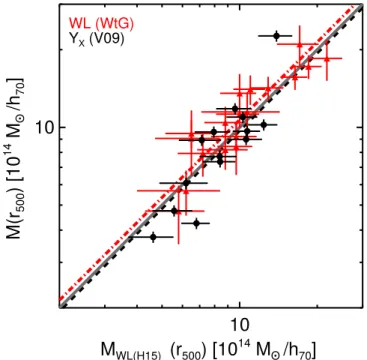
In Figure 1, we compare WL-based mass estimates from
H15 to YX-based mass estimates and to weak-lensing masses
from WtG. We have remeasured YX from archival Chandra
X-ray data for the 14 clusters fromH15with sufficiently deep X-ray measurements, which we use to estimate a cluster mass (MYx) using the YX-mass scaling relation from V09. For these
clusters, we also remeasure the deprojected weak-lensing aperture mass from the H15data set using the X-ray implied
r500. Using the X-ray implied r500 approximates what would
happen if the WL mass estimates were included in a joint YX–
WL scaling relationfit because of the relatively low scatter of YXwith cluster mass and, as we will show later, the agreement
in the resulting YX–M relation. To compareH15and WtG mass
estimates at the same radius, we extract a WtG mass for each of the 18clusters in common at the value of r500implied by the
H15analysis. We specifically use the mass estimates computed by fitting an NFW model to the observed shear profiles from the WtG“color-cut” method (Applegate et al. 2014).
In Table 2, we give three different measures of the relative cluster mass estimates betweenH15, WtG, and V09. First, we
fit a scaling relation of the formln(MWL)=A+ln(MYx) with
a free log-normal intrinsic scatter, using the Bayesian linear regressionfitting code from Kelly (2007). For comparison, we
also estimate the bootstrap mean and median of the log of the mass ratio, which makes no assumption about the underlying scatter.
First considering the mass ratio betweenH15and V09, we find all three estimates imply a mass ratio near unity with the scaling relation, bootstrap mean, and bootstrap median, giving ratios of 1.01±0.07, 1.03±0.06, and 1.12±0.05, respec-tively. This implies that the YX-based masses from V09 are in
relatively good agreement with H15, with the H15 masses ∼1%–12% larger, depending on how the mass ratio is estimated. Next, we consider the mass ratio between WtG and H15. We also find that all three estimates imply a mass ratio near unity with the scaling relation, bootstrap mean, and bootstrap median giving ratios of 1.06±0.07, 1.07±0.07, and 1.11±0.05, respectively. Therefore the WL-based mass estimates from H15 and WtG are also in relatively good agreement, with the WtG masses∼6%–11% larger, comparable to the 7% estimated systematic uncertainty from H15. The overlapping cluster sample between our V09-YX sample and
WtG is smaller (eight clusters), and therefore has larger
Figure 1. A plot comparing cluster weak lensing and YX-based mass estimates. Plotted along the y-axis are weak lensing-based mass estimates from WtG(red) and YX-based mass estimates using the scaling from V09(black). On the x-axis are weak lensing-based mass estimates from H15. For the H15/V09 comparison(black points), we have re-estimated theH15masses using the X-ray implied r500. The solid grey line shows a one-to-one relation, and the dashed black and red lines give the normalization implied for the bootstrap meanfit to the ratio of the masses (for details see text).
Table 2
Mass Ratios between Weak Lensing(H15, WtG) and YX(V09) Based Mass Estimates
Data set Nclust Log-normal Mean Median
H15/V09 14 1.01±0.07 1.03±0.06 1.12±0.05
WtG/H15 18 1.06±0.07 1.07±0.07 1.11±0.05
WtG/V09 8 1.15±0.10 1.17±0.13 1.24±0.09
50
This equation differs slightly fromB13andR13in order to more rigorously scale the V09 results if BX¹0.6 and h¹0.72 simultaneously. This modification has a negligible effect on any of the results in this work.
uncertainty on the mass ratio. Wefind that the three different mass ratio estimates between WtG and V09 range from 1.15–1.24. This range is somewhat larger than, but comparable with, the expectation when considering the mass ratios of the larger samples used to calculate the WtG/H15and H15/V09
mass ratios, which would predict a mass ratio between WtG and V09 of ∼1.1–1.2.
In summary, comparing to the original YX–M calibration
from V09, we find that the WL measurements imply a normalization that increases the YX-based cluster masses by a
factor between 1.0 and 1.2, depending on the WL analysis and data set (H15, WtG), and the fit assumptions. We therefore choose a Gaussian prior on the normalization of our YX–M
relation of AX=6.350.61, which increases the normal-ization from V09 by a factor of 1.1 with an overall uncertainty of 10%. We expect that this uncertainty includes the sum of our statistical and systematic uncertainty, because it brackets the range of values in the above comparison with the WL measurements and is comparable to our naive expectation given the statistical uncertainty in the fit above and the systematic uncertainty estimated inH15. This effectively gives us a purely WL-derived mass scale, independent of the hydrostatic mass estimates. We expect our constraints on the mass scale to improve in future work using WL observations of SPT-SZ survey clusters, which we will then be able to directly include in our cosmological analysis.
Finally, we have also estimated the dependence of the weak-lensing and X-ray-derived mass estimates on cosmological parameters. Over the range of cosmological parameters explored, the ratio of the two varies negligibly compared to the uncertainty of 10%.
5. COSMOLOGICAL ANALYSIS
Armed with the abundance of clusters as a function of the observables z, ξ, and YX, and models of the scaling of these
observables with cluster mass, we are almost ready to place constraints on the cosmological parameters. For thefinal step, we need a theoretical framework for translating the cosmolo-gical parameters into a prediction for the number of clusters as a function of mass and redshift, and we need a statistical method for comparing those predictions to our observed abundance. For both of these requirements, we closely follow the methods ofV10,B13, andR13.
5.1. Parameters to Cluster Abundance Predictions For a given set of cosmological parameters, we use the Code for Anisotropies in the Microwave Background(CAMB, Lewis et al.2000) to generate the matter power spectrum as a function
of redshift. We use this power spectrum as input to the Tinker et al. (2008) halo mass function, with which we calculate the
number of dark matter halos as a function of spherical overdensity mass M500and redshift.
More recent results(e.g., Bhattacharya et al.2011; Skillman et al.2014) confirm that, over the range of cluster masses and
redshifts considered in this work, the Tinker mass function is accurate to a level that is more than sufficient for the cosmological parameter constraints presented. For instance, even a shift as large as 10% in the halo mass function at
~ ´
M500 3 1014M would only affect the cosmological
constraints presented in Section 6.2at the 0.2slevel.
Given the Tinker mass function, we relate the cluster mass to the observed quantities ξ and YX using the scaling relations
described in Sections2.1.1and4.1.
In our default cosmological analysis, we use the standard six-parameter ΛCDM model, parameterized by the physical densities of baryons and cold dark matter at z=0, W hb 2 and
W hc 2, the angular scale of the sound horizon at last scattering qs,
the tilt of the scalar power spectrum ns, the amplitude of the
scalar power spectrum As, and the optical depth to reionization
τ. We will often refer to values of parameters derived from combinations of these original six, such as s8, the amplitude of
linear matterfluctuations on 8Mpc/h scales at z=0, Wm, the
total matter density at z=0, and H0=100 km sh -1Mpc-1, the value of the Hubble parameter at z=0. We explore three extensions toΛCDM. We first explore a model in which the sum of the neutrino masses Sm is a free parameter. In thisn
work we use the prescription from Costanzi et al. (2013) to
predict the effect of massive neutrinos on the halo mass function. We also consider a cosmological model in which Smn
and Neff, the effective number of relativistic particle species, are
both free parameters, and a model in which w, the parameter describing the equation of state of dark energy, is allowed to vary.
5.2. Cluster Likelihood Evaluation
To compare theoretical predictions for cluster abundance to the observations in this work, we closely follow the likelihood derivation of V10, B13, and R13. We differ from those analyses in this work by presenting an efficient numerical technique that scales linearly rather than exponentially with the number of mass proxies.
As is appropriate for a cluster abundance measurement(Hu & Kravtsov 2003; Holder 2006), we start with the binned
Poisson statistic in cluster observable space, which consists of redshift z and an arbirary number of mass proxies. In this work, we use the SZ mass proxy ξ which was described in Section 2.1.1, and the X-ray mass proxy YX as described in
Section4.1. For a given observable-space bin xi, the probability
of observing n events, with expectation value y x( ) isi
= -P e y x n . 5 i y x i n i ( ) ! ( ) ( )
We choose to take the limit of small bins where y becomes arbitrarily small at all xi, and n is zero except at the locations of
xiwhere clusters have been observed(Mantz et al.2008,2010,
V09). If we let xjdenote the bin that contains the jth cluster, we
obtain =
å
P = -å
y x +å
y x ln ln ln , 6 i i i i j j ( ) ( ) ( )where i runs over all observable space bins, and j runs over detected clusters. In this work, we are dealing specifically with the three-dimensional cluster observable space {z, ,x YX}, so
we can write the model expectation value
x
=
y x( )i N z( i, i,YX,i) and express the likelihood as
å
å
x x = -+ N z Y N z Y ln , , ln , , , 7 i i i i i i j j j j , , X, X, 1 2 3 1 2 3 ( ) ( ) ( )where the i i1, 2,i3sums again run over all possible values and j
only runs over the bins where clusters were detected. Going to the continuous limit would result in a divergent likelihood expression. This can be understood by the fact that the model is increasingly unlikely to produce our particular realization of the cluster catalog as we go tofiner binning. The divergence can be removed by simply adding - D D Dln z x YX to Equation (7).
This quantity (the logarithm of the observable-space bin volume) depends only on the choice of bin size, so that
D ln for different values of cosmological or scaling relation parameters remains meaningful. This procedure corresponds to substituting the number density dN z( , ,x YX) dzd dYx Xfor the
number contained in a bin N z(j,xj,YX,j). We then obtain the
expression
ò
å
x x x x x = -+ dzd dY dN z Y dzd dY dN z Y dzd dY ln , , ln , , . 8 j j j j X X X X, X ( ) ( ) ( )V10,B13, andR13evaluated this expression on either a two-dimensional or three-two-dimensional uniformly spaced grid. Each dimension was gridded into several hundred points, so that the computational cost rises exponentially with the number of mass proxies. The computational cost was trivial for V10, challen-ging forB13andR13, and likely intractable in future work if another mass proxy is added. The techniques used in Mantz et al. (2010) and Vikhlinin et al. (2009b) also scale
exponentially with the number of mass proxies.
Instead of computing Equation (8) on a uniformly spaced
grid, we use the following numerical techniques. First, we note that the follow-up mass proxy YXimmediately integrates out of
the first term. This applies to any mass proxy that does not appear in the survey selection function. Therefore, we only need to perform a two-dimensional integral
ò
x xò
ò
x x x - = -x ¥ ¥ dzd dY dN z Y dzd dY dz d dN dzd , , . 9 z X X X cut cut ( ) ( ) We evaluate this expression withò
ò
ò
ò
x x x x = > x ¥ ¥ ¥ ¥ dz d dN dzd dz dM dN dzdMP M , 10 z z 0 cut cut cut cut ( ∣ ) ( )where P(x>xcut∣M) is simply the significance cut modeled
through the scaling relation as described in Section2.1.1. The second term of Equation (8) is more challenging to
evaluate. It can be written as an integral over the mass function,
ò
x x x x x x = ¢ á ñ ´ ¢ á ñ ´ ¢ á ñ ¢ ¢ ¢ dN z Y dzd dY dz d dY d M P z z P P Y Y P z Y z M dN dzd M , , ln , , , ln ln . 11 j j j j j j X, X X X, X X ( ) ( ∣ ) ( ∣ ) ( ∣ ) ( ∣ ) ( )The probability density functions P z z( ∣ ),j ¢ P( ∣x xjá ñ), and ¢
P Y( X,j∣YX) describe the (independent) measurement error of
each of the observables. P z( ¢ á ñ, x ,YX¢∣z, lnM) describes the
joint scaling relations, implemented with multi-dimensional log-normal intrinsic scatter. In our case of two mass proxies(ξ,
YX), this is implemented with three parameters: two describing
the marginal variances slnz and sYx, as well as one correlation
coefficient rz,Yx, each of which is marginalized over in this work. Due to the treatment of maximization bias in Section 2.1.1, the scaling relation is defined in terms of ζ rather than xá ñ. We perform the change of variables using
⎜ ⎟ ⎛ ⎝ ⎞ ⎠
ò
x z z x z z ¢ á ñ ¢ = ¢ ¢ - á ñ - ¢ ¢ ¢ ¢ P z Y z M d P z Y z M , , X , ln 1 exp 1 2 , , X , ln . 12 2 ( ∣ ) ( ) ( ∣ ) ( )The computational bottleneck for evaluating the cluster likelihood lies in evaluating Equation (11). We use Monte
Carlo integration, randomly drawing from the probability distribution P z z( ∣ )j ¢ P( ∣x xjá ñ) P Y( X,j∣Y X¢)
x
¢ á ñ ¢
P z( , ,YX , ln∣z M), weighted by the mass function ddNlnM. Letlnmk¢denote the kth integration variable corresponding to
its flat-prior mass estimate (i.e., z¢ andY X substituted into¢
their respective observable-mass scaling relations). We can then write ⎛ ⎝ ⎜ ⎞ ⎠ ⎟
å
p ¢ ¢ = Y - ¢ - ¢ Y- ¢ - ¢ P m M m M m M ln ln 1 2 exp 1 2 ln ln ln ln , 13 k N l k 1kl l obs ( ∣ ) ( ) ∣ ∣ ( )( ) ( ) ( ) where Y is the mass proxy covariance matrix containing the intrinsic scatter and correlation coefficient parameters intro-duced in Sections 2.1.1 and 4.1 so that Y = ákl (lnmk¢–lnM¢)(lnml¢–lnM¢ ñ) .Now, we wish to obtain samples of the integration variable ¢
M
ln , given the location at which we are attempting to evaluate
dN x( )j dx. In order to efficiently draw samples we first, for
each k, draw samples from the (inverse) measurement error ¢
P x( k j,∣ ), which is assumed to be independent for each k. Wexk
then substitute these values into the scaling relations to obtain an ensemble oflnmk¢values. The remaining task is then to draw
random deviates lnM¢ that follow the probability distribution explicitly shown in Equation (13), given each value oflnmk¢.
To do so, we note that
S ¢ - ¢ ¢ - ¢ Y = S ¢ ¢ Y - ¢S ¢S Y + ¢ S Y = - ¢ + ¢ = + -- ¢ -m M m M m m M m M T T M T M T ln ln ln ln ln ln 2 ln ln ln 2 ln ln , 14 kl k l kl kl k l kl k k l kl kl kl M T T T T T 1 1 1 2 1 0 1 2 2 ln 1 2 0 1 2 2 12 2
(
)
( )( )( ) ( ) ( ) ( ) ( ) whereT0= Skllnmk¢lnml¢ Y( -1) ,kl T1= Sklnmk¢S Yl( -1) , andkl = S Y-T2 kl( 1) ,kl which is quadratic in lnM¢, so that
Equation(13) is a log-normal distribution in ¢M with a known
mean, width and normalization. We compute T0, T1, and T2
Having obtained samples of lnM¢, which we denote as ¢
M
ln ˜ , we average the mass function
å
p p ¢ - -Y ¢ N dN d M T T 1 ln 2 exp 2 15 i M T T N samples ln 2 1 2 0 i 12 2 obs(
)
( ) ∣ ∣ ( ) ˜and combine with Equation (14) to obtain an estimate for
Equation(11). Our implementation of this estimator has been
demonstrated to be unbiased through extensive simulations, with well-behaved residuals. The error on the mean is found to decrease as the inverse square root of the number of deviates drawn. In practice, for two mass proxies and 377 cluster candidates, we draw 104 deviates per cluster candidate, resulting in rms noise on the likelihood surface of
D -2 ln( ) 0.1 near the maximum likelihood. For the cluster catalog used in this work, the execution time is approximately one second on a single CPU thread. This likelihood module has been checked against an independent implementation, based on the estimator presented in Bocquet et al.(2015). The comparison shows agreement to well within
the 1σ uncertainties on the cosmological parameter constraints found in this work.
5.3. External Data sets
In Section 6, we will discuss the cosmological constraints obtained using the analysis laid out so far. We will evaluate the compatibility of the cluster data with other data sets, as well as show the improvements in parameter constraints when the cluster data set is combined with other data sets. The primary external data we use are CMB power spectrum measurements, measurements of BAO from galaxy surveys, and distances to Type Ia supernovae (SNe).
The canonical CMB power spectrum data we use is the temperature–temperature power spectrum from the Planck 2013 release, combined with low-ℓ polarization information from WMAP (Planck Collaboration et al. 2014a, hereafter Planck+WP). The qualitative results from this work will be very similar to those that would have been obtained by considering the Planck 2015 data set, since the constraints on
s8 and Wm from the temperature and low-ℓ polarization power
spectrum are very similar between the two Planck releases. In Section6.2, we will briefly review the effect of substituting the best CMB power spectrum data from before the Planck 2013 release, using instead the combination of WMAP9 (Hinshaw et al. 2013) and SPT (Story et al. 2013, hereafter S13) CMB
power spectrum data.
We sometimes use a prior on the angular scale of the sound horizon qs. This is a powerful piece of cosmological
information, and relies only very weakly on the details of the CMB analysis, since it affects the peak positions. We use the Planck+WP measurement, though we conservatively increase the uncertainty by a factor of five to
q =
100 MC 1.0413 0.0034.51 Since qs is so well-measured,
none of the results presented in this work that use a prior on qs
are sensitive to the specific value of the assumed uncertainty. When BAO data are used in this work, we use the SDSS-III BOSS results from data release 11. Specifically, we use the
measurements of the parameter combination DV rsat z=0.32
(LOWZ) and z=0.57 (CMASS) from Anderson et al. (2014).
When considering cosmologies with a free parameter describing the dark energy equation of state, we compare to and contrast with the SN results from the joint likelihood analysis of the SDSS-II and SNLS SN samples from Betoule et al.(2014).
Cluster abundances do weakly constrain the baryon density, but for our main results we choose to adopt a prior based on big-bang nucleosynthesis calculations and deuterium abun-dance measurements of Wbh2 =0.022020.00045 (Cooke et al.2014). Rather than fixing this parameter, we marginalize
over the uncertainty, though that analysis choice has no significant effect on the results presented in this work.
Finally, where stated, we adopt a prior of
= -
-H0 73.8 2.4 km s 1Mpc 1 from the direct H0
measure-ments of Riess et al.(2011). We find that changing this prior by
s
1 affects the resulting s8 constraint by 0.2 , while the Ws m
constraint is affected by ~0.4 . These two effects are anti-s correlated so that the commonly used parameter combination
s W 0.278( m )0.3 is highly insensitive to the assumed value
of H0.
6. COSMOLOGICAL CONSTRAINTS
In this section, we discuss the parameter constraints obtained using the data and methods described in the previous sections. We first explain which parameters and combinations of parameters are most strongly constrained by cluster abundance measurements. We then discuss the constraints from this cluster sample, both in comparison to and in combination with other cosmological data sets, for different choices of cosmological models. We assume spatialflatness throughout this work.
6.1. Parameter Sensitivity to Cluster Abundance A measurement of cluster abundance as a function of redshift provides constraints on cosmological parameters through several mechanisms. First, the total number of clusters found strongly depends on the matter density and the amplitude of the matter power spectrum (e.g., Bahcall & Cen 1992; White et al. 1993). As shown in, e.g., White et al. (1993), a simple
spherical-collapse model for the halo mass function(Press & Schechter 1974) indicates that the total number of clusters
should most strongly constrain the parameter combination
s Wa m
8 , whereα is related to the local slope of the matter power
spectrum at the mean mass of the cluster catalog. This prediction has been empirically borne out in many cluster abundance studies, including this one.
The redshift dependence of the cluster abundance contains information on the growth function, as well as a dependence on the cosmic volume surveyed. This combination of sensitivity to growth and volume provides a unique constraint on parameters that affect the expansion history, notably w, the equation of state of dark energy(e.g., Haiman et al.2001). In the case of w,
the effect of changing this parameter on the cluster abundance actually changes sign atz~1(e.g., Figure 1 of Mohr2005).
The 377 cluster candidates presented in this work provide a large enough sample to constrain cosmological parameters by measuring the evolution of cluster abundance. However, this constraint is also potentially limited by knowledge of the observable-mass scaling relations, in this case their evolution
51 q
with redshift. This is further discussed in the context of dark energy in Section 6.5.
In addition to their effect on the true abundance of clusters as a function of mass and redshift, cosmological parameters also affect the cluster observables through their influence on the SZ and X-ray scaling relations. Specifically, while the mass estimate inferred from the ζ–M relation depends weakly on redshift, the mass estimate inferred from the YX–M scaling
relation depends strongly on the angular diameter distance to the cluster.
6.2. ΛCDM
In this section, we present constraints on the parameters of theΛCDM model. Because not all parameters of this model are well constrained by cluster counts alone, we adopt priors on some of the six cosmological parameters(W hb 2, W hc 2, qs, ns, As,
and τ, defined in Section5.1), in addition to the priors on the
scaling relation parameters(ASZ, BSZ, CSZ, and slnz, described
in Section 2.1.1, as well as AX, BX, CX, slnYx, and rz,Yx,
described in Section 4.1). The cluster likelihood is insensitive
to the optical depth to reionizationτ as well as to the primordial scalar spectrum power-law index ns, once an appropriate pivot
point is chosen. Therefore, when discussing cluster constraints without the inclusion of CMB temperature power spectrum data, wefix these parameters to the best-fit values from Planck Collaboration et al. (2014a).
These two prior constraints, in addition to the H0and BBN
priors discussed in 5.3, leave us two remaining degrees of freedom in theΛCDM model, which we choose to express as Wm and s8 (though in exploring the likelihood surface we
actually vary the base parameters W hb 2, W hc 2, ln 1010As and
H0). We fix the species-summed neutrino mass Smn to
0.06eV, the minimum allowed value from terrestrial measure-ments of squared neutrino mass differences(see e.g., Gonzalez-Garcia et al.2012for a review). Figure2shows the constraints
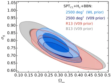
on s8and WmfromB13,R13, and this work. The large increase
in the number of clusters primarily reduces the uncertainty on Wm by constraining the shape of the halo mass function. The
uncertainty on the parameter combination s W8( m 0.27)0.3is set by the knowledge of the overall mass scale, rather than the number of clusters, since Poisson errors on this number are subdominant. The improvement in the s W8( m 0.27)0.3 con-straint results from the increase in the number of clusters with Chandra follow-up data. These two effects result in tighter joint constraints on the two parameters than we obtained in previous cluster analyses, if we use the same prior on the observable-mass relations. This can be seen in Figure 2: the innermost, purple contours use the current cluster sample and the same observable-mass priors asB13andR13. However, in contrast toB13andR13we choose to use a WL-based prior on the overall mass scale for our baseline results, as discussed in
4.2. This results in slightly degraded constraints, in particular on s8, as can be seen from the light-blue contours in Figure2.
With the current cluster sample, the stated priors on cosmological parameters, and the updated priors on the observable-mass relations, we obtain
s =8 0.7840.039, (16) W =m 0.2890.042, (17) and
s W8( m 0.27)0.3=0.7970.031. (18) The ΛCDM parameter constraints, including scaling relation parameters, are shown in Table3.
In the left- and right-hand panels of Figure 3 we show the cluster abundance as a function of redshift and detection significance, respectively. Both show one-dimensional repre-sentations of the observable-space mass function. The data points, with approximate ( N ) error bars shown, are independent of cosmological and scaling relation parameters. The points are independent between bins fordN d , and nearlyx
independent for dN/dz, where clusters without spectroscopic redshift information can contribute to multiple bins.
Shifts in the parameters s8and ASZresult in roughly global
shifts in the amplitude of both curves, simultaneously. The scaling relation parameter BSZinduces a roughly power-law tilt
indN d , and parameters such as Cx SZand Wm induce tilts in
dN/dz. This visualization shows two important ways in which the model, marginalized over a large number of scaling relation and cosmological parameters, is tested for agreement with the data.
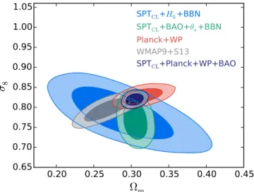
Figure4shows the cluster constraints on theΛCDM model in the s8-Wm plane, when combined with either the H0+BBN
prior or the BAO q+ s+BBN prior. We also show the constraints
from CMB power spectrum measurements from Planck+WP and WMAP9+S13data. The 68% confidence regions from the cluster constraints and the CMB power spectrum constraints overlap. We proceed to adopt the Planck+WP data set as the baseline CMB data set for the remainder of this work. We also combine the SPTCL+Planck+WP+BAO data sets to obtain
jointΛCDM parameter constraints. Finally, we note that the s8
constraint obtained using the SPTCL data in Table3 is within s
1 of the value recently reported by the Planck collaboration for the full-mission data (their 2015 TT+lowP+lensing data set) of s =8 0.8150.009.
Figure 2. Comparison of cluster constraints on s8and Wmfrom this work with
those from previous SPT publications. The B13 analysis (outermost, gray contours) used 18clusters, 14of which have Chandra observations. The number of clusters increased to 100inR13(red contours), whereas this work uses 377 cluster candidates, 82 of which have high-quality Chandra observations. If we adopt the same observable-mass priors asB13andR13, we obtain the innermost, purple contours. However, the main results in this paper assume a new weak lensing-based prior on the X-ray scaling relation normalization, which changes the central value by 10% and increases the 1σ uncertainty slightly from 9% to 11%. The s8-Wmconstraints using this prior and
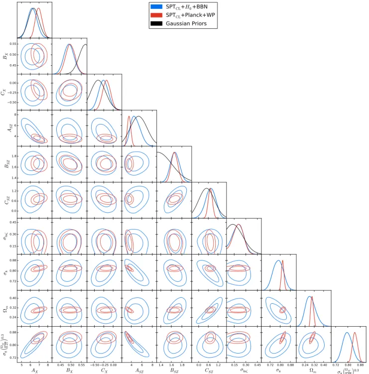
6.2.1. Constraints on Scaling Relation Parameters While the main focus of this work is on the cosmological constraints, the nuisance parameters are of interest themselves, both in terms of the cluster scaling relation parameter constraints and their degeneracy with the cosmological parameters. In Figure 5, we show the marginalized posterior in the multi-dimensional parameter space.
The dominant systematic uncertainty limiting the cosmolo-gical constraints from the SPT-SZ cluster sample is the uncertainty of the overall cluster mass scale. This can be seen as a strong degeneracy between AXand s W8( m 0.27) , which0.3
are 85% correlated given the SPTCL+H0+BBN data set. The
second most important source of systematic uncertainty in the cosmological constraints is from the parameter characterizing the redshift evolution of the scaling relation, CSZ. In aΛCDM
cosmology, it is highly degenerate with Wm, correlated at 87%
when considering the SPTCL+H0+BBN data set.
The parameters that shift most significantly away from their priors are the BSZand BXparameters which encode the
power-law slopes of the scaling relations. Wefind that the preference for high BSZ persists when the X-ray data are not used. In
addition, this preference is not localized to any particular region of the data; when considering half the cluster sample at a time, either by redshift,ξ, or gfield, the high BSZpersists, albeit at a
lower significance.
This high BSZ implies that the measured observable-space
mass function, dN dx, is shallower than expected given the scaling relation found from the simulations described in Section 2.2. We can approximately quantify this by assuming
x
dN d follows a power law. The data prefer a power-law index
of∼4.0, compared to the simulation prediction of ∼5.0, which is disfavored by the measureddN dx at~4.5 .s
The preference for a higher BSZ, i.e., a steeperζ–M relation,
is statistically weak, approximately s1 , due to the relatively weak 20% width assumed on the BSZ prior. By contrast, the
assumed width of the prior on the X-ray scaling relation slope BXis 5%, leading to a tension between the likelihood and the
prior of approximately 4 . There is some evidence for as similarly steep YX–M scaling relation from the comparison of
the V09 andH15WL mass estimates in Figure1, which prefers ~
BX 0.42. Such a slope would be in ~4 tension with thes expected self-similar cluster slope of BX=0.6.
In this work, we will assume that our observational priors on the YX–M slope and theoretical priors on the mass function
slope are well motivated, but note that the shape of the
observable-space mass function will need to be studied in more detail for future work.
6.3.ΛCDM + Smn
We now consider a cosmological model in which the species-summed neutrino mass Smn is a free parameter.
Constraints on this model from the CMB power spectrum show a strong degeneracy between s8and Smn(e.g., Komatsu
et al. 2009; Planck Collaboration et al. 2014a; Abazajian et al.2015). This allows even modest measurements of s8 to
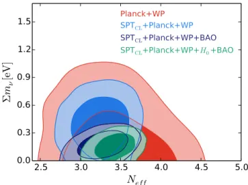
improve on neutrino mass constraints from the CMB power spectrum data alone. Figure 6 shows the improvement in constraints when adding cluster abundance information to CMB power spectrum data alone(Planck+WP), and also when including BAO data. In both cases, the addition of cluster information tightens the constraint and causes the posterior to peak at positive values of Sm , though the 95% upper limit onn
Sm remains largely unchanged. Allowing the Sn m to vary inn
the range of 0–2eV, and using the combination of the SPTCL+Planck+WP+BAO data sets, we find
Smn=0.14 0.08eV. (19) We note that the preference for positive Sm , when wen
combine our cluster abundance measurements with Planck data, is driven by the small residual tension between the preferred values of s8 in the two data sets. Such a preference
has been pointed out by several authors(e.g., Battye & Moss
2014; Planck Collaboration et al.2014b; Wyman et al.2014),
but is in contrast to the preference for positive Sm shown, forn
example, by the combination of WMAP+SPT CMB power spectrum data and SPT cluster data in Hou et al. (2014), in
which the evidence for positive Sm is not driven by the clustern
data. In this work, wefind relatively good agreement between the preferred s8 using the CMB and SPTCL data sets, so the
preference for positive Sm is weak and consistent at 1n σ with
the minimum expected value of ∼0.06 eV from neutrino oscillation experiments(Lesgourgues & Pastor2006). Relative
to the previous cluster-based constraints cited above, the updated WL-based calibration described in Section 4.2, has shifted the normalization and increased the uncertainty of the observable-mass relation in a way that relieves tension with the Planck CMB data (see Figure 2). We also note that our
constraint on Sm is largely independent of the change in then
optical depth to reionization, τ, between the Planck 2013 and 2015 data release; the SPTCL constraints are independent ofτ, Table 3
Constraints on Cosmological and Scaling Relation Parameters Assuming aΛCDM Cosmology
Parameter Prior SPTCL+H0+BBN SPTCL+BAO+BBN SPTCL+Planck+WP+BAO
ASZ 5.38±1.61 4.842±0.913 4.936±0.955 3.531±0.273 BSZ 1.340±0.268 1.668±0.083 1.660±0.064 1.661±0.060 CSZ 0.49±0.49 0.550±0.315 0.864±0.159 0.733±0.123 slnz 0.13±0.13 0.199±0.069 0.201±0.070 0.203±0.066 AX 6.38±0.61 6.235±0.514 6.316±0.505 7.030±0.341 BX 0.57±0.03 0.491±0.023 0.493±0.023 0.498±0.021 CX −0.40±0.20 −0.251±0.127 −0.280±0.122 −0.174±0.102 slnYx 0.12±0.08 0.162±0.070 0.160±0.069 0.154±0.064 rz,Yx [-0.98, 0.98] −0.147±0.458 −0.136±0.465 −0.204±0.443 Wm L 0.289±0.042 0.306±0.010 0.304±0.007 s8 L 0.784±0.039 0.768±0.030 0.820±0.009 s W 0.278( m )0.3 L 0.797±0.031 0.797±0.030 0.850±0.013