AND COOPERATION* ERNSTFEHR AND KLAUSM. SCHMIDT
There is strong evidence that people exploit their bargaining power in competitive markets but not in bilateral bargaining situations. There is also strong evidence that people exploit free-riding opportunities in voluntary cooperation games. Yet, when they are given the opportunity to punish free riders, stable cooperation is maintained, although punishment is costly for those who punish. This paper asks whether there is a simple common principle that can explain this puzzling evidence. We show that if some people care about equity the puzzles can be resolved. It turns out that the economic environment determines whether the fair types or the selfish types dominate equilibrium behavior.
I. INTRODUCTION
Almost all economic models assume that all people are exclusively pursuing their material self-interest and do not care about ‘‘social’’ goals per se. This may be true for some (maybe many) people, but it is certainly not true for everybody. By now we have substantial evidence suggesting that fairness motives affect the behavior of many people. The empirical results of Kahneman, Knetsch, and Thaler [1986], for example, indicate that customers have strong feelings about the fairness of firms’ short-run pricing decisions which may explain why some firms do not fully exploit their monopoly power. There is also a lot of evidence suggesting that firms’ wage setting is constrained by workers’ views about what constitutes a fair wage [Blinder and Choi 1990; Agell and Lundborg 1995; Bewley 1995; Campbell and Kamlani 1997]. According to these studies, a major reason for firms’ refusal to cut wages in a recession is the fear that workers will perceive pay cuts as unfair which in turn is expected to affect work morale ad-versely. There are also many well-controlled bilateral bargaining experiments which indicate that a nonnegligible fraction of the
* We would like to thank seminar participants at the Universities of Bonn and Berlin, Harvard, Princeton, and Oxford Universities, the European Summer Symposium on Economic Theory 1997 at Gerzense´e (Switzerland), and the ESA conference in Mannheim for helpful comments and suggestions. We are particu-larly grateful to three excellent referees and to Drew Fudenberg and John Kagel for their insightful comments. The first author also gratefully acknowledges support from the Swiss National Science Foundation (project number 1214-05100.97) and the Network on the Evolution of Preferences and Social Norms of the MacArthur Foundation. The second author acknowledges financial support by the German Science Foundation through grant SCHM 119614-1.
r1999 by the President and Fellows of Harvard College and the Massachusetts Institute of
Technology.
subjects do not care solely about material payoffs [Gu¨ th and Tietz, 1990; Roth 1995; Camerer and Thaler 1995]. However, there is also evidence that seems to suggest that fairness considerations are rather unimportant. For example, in competitive experimen-tal markets with complete contracts, in which a well-defined homogeneous good is traded, almost all subjects behave as if they are only interested in their material payoff. Even if the competi-tive equilibrium implies an extremely uneven distribution of the gains from trade, equilibrium is reached within a few periods [Smith and Williams 1990; Roth, Prasnikar, Okuno-Fujiwara, and Zamir 1991; Kachelmeier and Shehata 1992; Gu¨ th, Marchand, and Rulliere 1997].
There is similarly conflicting evidence with regard to coopera-tion. Reality provides many examples indicating that people are more cooperative than is assumed in the standard self-interest model. Well-known examples are that many people vote, pay their taxes honestly, participate in unions and protest movements, or work hard in teams even when the pecuniary incentives go in the opposite direction.1This is also shown in laboratory experiments
[Dawes and Thaler 1988; Ledyard 1995]. Under some conditions it has even been shown that subjects achieve nearly full cooperation, although the self-interest model predicts complete defection [Isaac and Walker 1988, 1991; Ostrom and Walker 1991; Fehr and Ga¨chter 1996].2However, as we will see in more detail in Section
IV, there are also those conditions under which a vast majority of subjects completely defect as predicted by the self-interest model. There is thus a bewildering variety of evidence. Some pieces of evidence suggest that many people are driven by fairness considerations, other pieces indicate that virtually all people behave as if completely selfish, and still other types of evidence suggest that cooperation motives are crucial. In this paper we ask whether this conflicting evidence can be explained by a single simple model. Our answer to this question is affirmative if one is willing to assume that, in addition to purely self-interested people, there are a fraction of people who are also motivated by fairness considerations. No other deviations from the standard
1. On voting see Mueller [1989]. Skinner and Slemroad [1985] argue that the standard self-interest model substantially underpredicts the number of honest taxpayers. Successful team production in, e.g., Japanese-managed auto factories in North America is described in Rehder [1990]. Whyte [1955] discusses how workers establish ‘‘production norms’’ under piece-rate systems.
2. Isaac and Walker and Ostrom and Walker allow for cheap talk, while in Fehr and Ga¨chter subjects could punish each other at some cost.
economic approach are necessary to account for the evidence. In particular, we do not relax the rationality assumption.3
We model fairness as self-centered inequity aversion. Ineq-uity aversion means that people resist inequitable outcomes; i.e., they are willing to give up some material payoff to move in the direction of more equitable outcomes. Inequity aversion is self-centered if people do not care per se about inequity that exists among other people but are only interested in the fairness of their own material payoff relative to the payoff of others. We show that in the presence of some inequity-averse people ‘‘fair’’ and ‘‘coopera-tive’’ as well as ‘‘competi‘‘coopera-tive’’ and ‘‘noncoopera‘‘coopera-tive’’ behavioral patterns can be explained in a coherent framework. A main insight of our examination is that the heterogeneity of preferences interacts in important ways with the economic environment. We show, in particular, that the economic environment determines the preference type that is decisive for the prevailing behavior in equilibrium. This means, for example, that under certain competi-tive conditions a single purely selfish player can induce a large number of extremely inequity-averse players to behave in a completely selfish manner, too. Likewise, under certain conditions for the provision of a public good, a single selfish player is capable of inducing all other players to contribute nothing to the public good, although the others may care a lot about equity. We also show, however, that there are circumstances in which the exis-tence of a few inequity-averse players creates incentives for a majority of purely selfish types to contribute to the public good. Moreover, the existence of inequity-averse types may also induce selfish types to pay wages above the competitive level. This reveals that, in the presence of heterogeneous preferences, the economic environment has a whole new dimension of effects.4
There are a few other papers that formalize the notion of fairness.5In particular, Rabin [1993] argues that people want to
be nice to those who treat them fairly and want to punish those who hurt them. According to Rabin, an action is perceived as fair if
3. This differentiates our model from learning models (e.g., Roth and Erev [1995]) that relax the rationality assumption but maintain the assumption that all players are only interested in their own material payoff. The issue of learning is further discussed in Section VII below.
4. Our paper is, therefore, motivated by a concern similar to the papers by Haltiwanger and Waldman [1985] and Russell and Thaler [1985]. While these authors examine the conditions under which nonrational or quasi-rational types affect equilibrium outcomes, we analyze the conditions under which fair types affect the equilibrium.
the intention that is behind the action is kind, and as unfair if the intention is hostile. The kindness or the hostility of the intention, in turn, depends on the equitability of the payoff distribution induced by the action. Thus, Rabin’s model, as our model, is based on the notion of an equitable outcome. In contrast to our model, however, Rabin models the role of intentions explicitly. We acknowledge that intentions do play an important role and that it is desirable to model them explicitly. However, the explicit model-ing of intentions comes at a cost because it requires the adoption of psychological game theory that is much more difficult to apply than standard game theory. In fact, Rabin’s model is restricted to two-person normal form games, which means that very important classes of games, like, e.g., market games and n-person public good games cannot be analyzed. Since a major focus of this paper is the role of fairness in competitive environments and the analysis of n-person cooperation games, we chose not to model intentions explicitly. This has the advantage of keeping the model simple and tractable. We would like to stress, however, that— although we do not model intentions explicitly—it is possible to capture intentions implicitly by our formulation of fairness prefer-ences. We deal with this issue in Section VIII.
The rest of the paper is organized as followed. In Section II we present our model of inequity aversion. Section III applies this model to bilateral bargaining and market games. In Section IV cooperation games with and without punishments are considered. In Section V we show that, on the basis of plausible assumptions about preference parameters, the majority of individual choices in ultimatum and market and cooperation games considered in the previous sections are consistent with the predictions of our model. Section VI deals with the dictator game and with gift exchange games. In Section VII we discuss potential extensions and objec-tions to our model. Section VIII compares our model with alterna-tive approaches in the literature. Section IX concludes.
II. A SIMPLE MODEL OF INEQUITYAVERSION
An individual is inequity averse if he dislikes outcomes that are perceived as inequitable. This definition raises, of course, the difficult question of how individuals measure or perceive the fairness of outcomes. Fairness judgments are inevitably based on a kind of neutral reference outcome. The reference outcome that is used to evaluate a given situation is itself the product of
compli-cated social comparison processes. In social psychology [Festinger 1954; Stouffer 1949; Homans 1961; Adams 1963] and sociology [Davis 1959; Pollis 1968; Runciman 1966] the relevance of social comparison processes has been emphasized for a long time. One key insight of this literature is that relative material payoffs affect people’s well-being and behavior. As we will see below, without the assumption that at least for some people relative payoffs matter, it is difficult, if not impossible, to make sense of the empirical regularities observed in many experiments. There is, moreover, direct empirical evidence for the importance of relative payoffs. Agell and Lundborg [1995] and Bewley [1998], for example, show that relative payoff considerations constitute an important con-straint for the internal wage structure of firms. In addition, Clark and Oswald [1996] show that comparison incomes have a signifi-cant impact on overall job satisfaction. They construct a compari-son income level for a random sample of roughly 10,000 British individuals by computing a standard earnings equation. This earnings equation determines the predicted or expected wage of an individual with given socioeconomic characteristics. Then they examine the impact of this comparison wage on overall job satisfaction. Their main result is that—holding other things constant—the comparison income has a large and significantly negative impact on overall job satisfaction.
Strong evidence for the importance of relative payoffs is also provided by Loewenstein, Thompson, and Bazerman [1989]. These authors asked subjects to ordinally rank outcomes that differ in the distribution of payoffs between the subject and a comparison person. On the basis of these ordinal rankings, the authors estimate how relative material payoffs enter the person’s utility function. The results show that subjects exhibit a strong and robust aversion against disadvantageous inequality: for a given own income xi, subjects rank outcomes in which a comparison
person earns more than xi substantially lower than an outcome
with equal material payoffs. Many subjects also exhibit an aversion to advantageous inequality although this effect seems to be significantly weaker than the aversion to disadvantageous inequality.
The determination of the relevant reference group and the relevant reference outcome for a given class of individuals is ultimately an empirical question. The social context, the saliency of particular agents, and the social proximity among individuals are all likely to influence reference groups and outcomes. Because
in the following we restrict attention to individual behavior in economic experiments, we have to make assumptions about reference groups and outcomes that are likely to prevail in this context. In the laboratory it is usually much simpler to define what is perceived as an equitable allocation by the subjects. The subjects enter the laboratory as equals, they do not know any-thing about each other, and they are allocated to different roles in the experiment at random. Thus, it is natural to assume that the reference group is simply the set of subjects playing against each other and that the reference point, i.e., the equitable outcome, is given by the egalitarian outcome.
More precisely, we assume the following. First, in addition to purely selfish subjects, there are subjects who dislike inequitable outcomes. They experience inequity if they are worse off in material terms than the other players in the experiment, and they also feel inequity if they are better off. Second, however, we assume that, in general, subjects suffer more from inequity that is to their material disadvantage than from inequity that is to their material advantage. Formally, consider a set of n players indexed by i僆 51, . . . , n6, and let x ⫽ x1, . . . , xndenote the vector of
mone-tary payoffs. The utility function of player i僆 51, . . . , n6 is given by
(1) Ui(x)⫽ xi⫺ ␣i 1 n⫺ 1
兺
j⫽i max5xj⫺ xi,06 ⫺ i 1 n⫺ 1兺
j⫽i max5xi⫺ xj,06,where we assume thatiⱕ ␣iand 0ⱕ i⬍ 1. In the two-player
case (1) simplifies to
(2) Ui(x)⫽ xi⫺ ␣imax5xj⫺ xi,06 ⫺ imax5xi⫺ xj,06, i ⫽ j.
The second term in (1) or (2) measures the utility loss from disadvantageous inequality, while the third term measures the loss from advantageous inequality. Figure I illustrates the utility of player i as a function of xjfor a given income xi. Given his own
monetary payoff xi, player i’s utility function obtains a maximum
at xj⫽ xi. The utility loss from disadvantageous inequality (xj⬎ xi)
is larger than the utility loss if player i is better off than player j(xj⬍ xi).6
6. In all experiments considered in this paper, the monetary payoff functions of all subjects were common knowledge. Note that for inequity aversion to be
To evaluate the implications of this utility function, let us start with the two-player case. For simplicity, we assume that the utility function is linear in inequality aversion as well as in xi.
This implies that the marginal rate of substitution between monetary income and inequality is constant. This may not be fully realistic, but we will show that surprisingly many experimental observations that seem to contradict each other can be explained on the basis of this very simple utility function already. However, we will also see that some observations in dictator experiments suggest that there are a nonnegligible fraction of people who exhibit nonlinear inequality aversion in the domain of advanta-geous inequality (see Section VI below).
Furthermore, the assumption␣iⱖ icaptures the idea that a
player suffers more from inequality that is to his disadvantage. The above-mentioned paper by Loewenstein, Thompson, and
behaviorally important it is not necessary for subjects to be informed about the final monetary payoffs of the other subjects. As long as subjects’ material payoff functions are common knowledge, they can compute the distributional implica-tions of any (expected) strategy profile; i.e., inequity aversion can affect their decisions.
FIGUREI
Bazerman [1989] provides strong evidence that this assumption is, in general, valid. Note that␣i ⱖ i essentially means that a
subject is loss averse in social comparisons: negative deviations from the reference outcome count more than positive deviations. There is a large literature indicating the relevance of loss aversion in other domains (e.g., Tversky and Kahneman [1991]). Hence, it seems natural that loss aversion also affects social comparisons.
We also assume that 0ⱕ i⬍ 1. iⱖ 0 means that we rule out
the existence of subjects who like to be better off than others. We impose this assumption here, although we believe that there are subjects with i ⬍ 0.7 The reason is that in the context of the
experiments we consider individuals withi⬍ 0 have virtually no
impact on equilibrium behavior. This is in itself an interesting insight that will be discussed extensively in Section VII. To interpret the restrictioni⬍ 1, suppose that player i has a higher
monetary payoff than player j. In this casei⫽ 0.5 implies that
player i is just indifferent between keeping one dollar to himself and giving this dollar to player j. If i ⫽ 1, then player i is
prepared to throw away one dollar in order to reduce his advan-tage relative to player j which seems very implausible. This is why we do not consider the caseiⱖ 1. On the other hand, there is no
justification to put an upper bound on␣i. To see this, suppose that
player i has a lower monetary payoff than player j. In this case player i is prepared to give up one dollar of his own monetary payoff if this reduces the payoff of his opponent by (1⫹ ␣i)/␣i
dollars. For example, if␣i⫽ 4, then player i is willing to give up
one dollar if this reduces the payoff of his opponent by 1.25 dollars. We will see that observable behavior in bargaining and public good games suggests that there are at least some individuals with such high␣’s.
If there are n⬎ 2 players, player i compares his income with all other n⫺ 1 players. In this case the disutility from inequality has been normalized by dividing the second and third term by n⫺ 1. This normalization is necessary to make sure that the relative impact of inequality aversion on player i’s total payoff is indepen-dent of the number of players. Furthermore, we assume for simplicity that the disutility from inequality is self-centered in the sense that player i compares himself with each of the other
7. For the role of status seeking and envy, see Frank [1985] and Banerjee [1990].
players, but he does not care per se about inequalities within the group of his opponents.
III. FAIRNESS, RETALIATION, ANDCOMPETITION: ULTIMATUM AND MARKET GAMES
In this section we apply our model to a well-known simple bargaining game—the ultimatum game—and to simple market games in which one side of the market competes for an indivisible good. As we will see below, a considerable body of experimental evidence indicates that in the ultimatum game the gains from trade are shared relatively equally while in market games very unequal distributions are frequently observed. Hence, any alterna-tive to the standard self-interest model faces the challenge to explain both ‘‘fair’’ outcomes in the ultimatum game and ‘‘competi-tive’’ and rather ‘‘unfair’’ outcomes in market games.
A. The Ultimatum Game
In an ultimatum game a proposer and a responder bargain about the distribution of a surplus of fixed size. Without loss of generality we normalize the bargaining surplus to one. The responder’s share is denoted by s and the proposer’s share by 1⫺ s. The bargaining rules stipulate that the proposer offers a share s 僆 [0,1] to the responder. The responder can accept or reject s. In case of acceptance the proposer receives a (normalized) monetary payoff x1⫽ 1 ⫺ s, while the responder receives x2⫽ s. In case of a
rejection both players receive a monetary return of zero. The self-interest model predicts that the responder accepts any s 僆 (0,1] and is indifferent between accepting and rejecting s ⫽ 0. Therefore, there is a unique subgame perfect equilibrium in which the proposer offers s⫽ 0, which is accepted by the responder.8
By now there are numerous experimental studies from differ-ent countries, with differdiffer-ent stake sizes and differdiffer-ent experimen-tal procedures, that clearly refute this prediction (for overviews
8. Given that the proposer can choose s continuously, any offer s⬎ 0 cannot be an equilibrium offer since there always exists an s8 with 0 ⬍ s8 ⬍ s which is also accepted by the responder and yields a strictly higher payoff to the proposer. Furthermore, it cannot be an equilibrium that the proposer offers s⫽ 0 which is rejected by the responder with positive probability. In this case the proposer would do better by slightly raising his price—in which case the responder would accept with probability 1. Hence, the only subgame perfect equilibrium is that the proposer offers s⫽ 0 which is accepted by the responder. If there is a smallest money unit⑀, then there exists a second subgame perfect equilibrium in which the responder accepts any s僆 [⑀,1] and rejects, s ⫽ 0 while the proposer offers ⑀.
see Thaler [1988], Gu¨ th and Tietz [1990], Camerer and Thaler [1995], and Roth [1995]). The following regularities can be consid-ered as robust facts (see Table I). (i) There are virtually no offers above 0.5. (ii) The vast majority of offers in almost any study is in the interval [0.4, 0.5]. (iii) There are almost no offers below 0.2. (iv) Low offers are frequently rejected, and the probability of rejection tends to decrease with s. Regularities (i) to (iv) continue to hold for rather high stake sizes, as indicated by the results of Cameron [1995], Hoffman, McCabe, and Smith [1996], and Slonim and Roth [1997]. The 200,000 rupiahs in the second experiment of Cameron (see Table I) are, e.g., equivalent to three months’ income for the Indonesian subjects. Overall, roughly 60–80 percent of the offers in Table I fall in the interval [0.4, 0.5], while only 3 percent are below a share of 0.2.
To what extent is our model capable of accounting for the stylized facts of the ultimatum game? To answer this question, suppose that the proposer’s preferences are represented by (␣1,1),
while the responder’s preferences are characterized by (␣2,2).
The following proposition characterizes the equilibrium outcome as a function of these parameters.
PROPOSITION 1. It is a dominant strategy for the responder to
accept any offer sⱖ 0.5, to reject s if
s⬍ s8(␣2)⬅ ␣2/(1⫹ 2␣2)⬍ 0.5,
and to accept s⬎ s8(␣2). If the proposer knows the preferences
of the responder, he will offer
(3) s*
5
⫽ 0.5 if1⬎ 0.5
僆 [s8(␣2),0.5] if1⫽ 0.5
⫽ s8(␣2) if1⬍ 0.5
in equilibrium. If the proposer does not know the preferences of the responder but believes that␣2is distributed according
to the cumulative distribution function F(␣2), where F(␣2)
has support [␣, ␣] with 0 ⱕ ␣ ⬍ ␣ ⬍ ⬁, then the probability (from the perspective of the proposer) that an offer s⬍ 0.5 is going to be accepted is given by
(4) p⫽
5
1 if sⱖ s8(␣)
F(s/(1⫺ 2s)) 僆 (0,1) if s8(␣) ⬍ s ⬍ s8(␣))
Hence, the optimal offer of the proposer is given by (5) s*
5
⫽ 0.5 if1⬎ 0.5 僆 [s8(␣), 0.5] if1⫽ 0.5 僆 (s8(␣), s8(␣)] if1⬍ 0.5. TABLE IPERCENTAGE OFOFFERS BELOW0.2AND BETWEEN0.4AND0.5
IN THEULTIMATUMGAME
Study (Payment method) Number of observations Stake size (country) Percentage of offers with s⬍ 0.2 Percentage of offers with 0.4ⱕ s ⱕ0.5 Cameron [1995] (All Ss Paid) 35 Rp 40.000 (Indonesia) 0 66 Cameron [1995] (all Ss paid) 37 Rp 200.000 (Indonesia) 5 57 FHSS [1994] (all Ss paid) 67 $5 and $10 (USA) 0 82 Gu¨ th et al. [1982] (all Ss paid) 79 DM 4–10 (Germany) 8 61 Hoffman, McCabe, and Smith [1996] (All Ss paid) 24 $10 (USA) 0 83 Hoffman, McCabe, and Smith [1996] (all Ss paid) 27 $100 (USA) 4 74 Kahneman, Knetsch, and Thaler [1986] (20% of Ss paid) 115 $10 (USA) ? 75a Roth et al. [1991] (random pay-ment method) 116b approx. $10 (USA, Slovenia, Israel, Japan) 3 70
Slonim and Roth [1997] (random pay-ment method) 240c SK 60 (Slovakia) 0.4d 75
Slonim and Roth [1997] (random pay-ment method) 250c SK 1500 (Slovakia) 8d 69 Aggregate result of all studiese 875 3.8 71
a. percentage of equal splits, b. only observations of the final period, c. observations of all ten periods, d. percentage of offers below 0.25, e. without Kahneman, Knetsch, and Thaler [1986].
Proof. If sⱖ 0.5, the utility of a responder from accepting s is U2(s)⫽ s ⫺ 2(2s⫺ 1), which is always positive for 2⬍ 1 and thus
better than a rejection that yields a payoff of 0. The point is that the responder can achieve equality only by destroying the entire surplus which is very costly to him if sⱖ 0.5; i.e., if the inequality is to his advantage. For s⬍ 0.5, a responder accepts the offer only if the utility from acceptance, U2(s)⫽ s ⫺ ␣2(1⫺ 2s), is
nonnega-tive which is the case only if s exceeds the acceptance threshold s8(␣2)⬅ ␣2/(1⫹ 2␣2)⬍ 0.5.
At stage 1 a proposer never offers s⬎ 0.5. This would reduce his monetary payoff as compared with an offer of s⫽ 0.5, which would also be accepted with certainty and which would yield perfect equality. If1⬎ 0.5, his utility is strictly increasing in s for all s ⱕ
0.5. This is the case where the proposer prefers to share his resources rather than to maximize his own monetary payoff, so he will offer s⫽ 0.5. If 1⫽ 0.5, he is just indifferent between giving
one dollar to the responder and keeping it to himself; i.e., he is indifferent between all offers s 僆 [s’(␣2), 0.5]. If 1 ⬍ 0.5, the
proposer would like to increase his monetary payoff at the expense of the responder. However, he is constrained by the responder’s acceptance threshold. If the proposer is perfectly informed about the responder’s preferences, he will simply offer s8(␣2). If the
proposer is imperfectly informed about the responder’s type, then the probability of acceptance is F(s/(1⫺ 2s)) which is equal to one if sⱖ ␣(1 ⫹ 2␣) and equal to zero if s ⱕ ␣/(1 ⫹ ␣). Hence, in this case there exists an optimal offer s僆 (s8(␣), s8(␣)].
QED Proposition 1 accounts for many of the above-mentioned facts. It shows that there are no offers above 0.5, that offers of 0.5 are always accepted, and that very low offers are very likely to be rejected. Furthermore, the probability of acceptance, F(s/(1⫺ 2s)), is increasing in s for s⬍ s8(␣) ⬍ 0.5. Note also that the acceptance threshold s8(␣2) ⫽ ␣2/(1⫹ 2␣2) is nonlinear and has some
intui-tively appealing properties. It is increasing and strictly concave in ␣2, and it converges to 0.5 if␣2=⬁. Furthermore, relatively small
values of␣2already yield relatively large thresholds. For example,
␣2⫽1⁄3implies that s8(␣2)⫽ 0.2 and ␣2⫽ 0.75 implies that s8(␣2)⫽
0.3.
In Section V we go beyond the predictions implied by Proposi-tion 1. There we ask whether there is a distribuProposi-tion of preferences
that can explain not just the major facts of the ultimatum game but also the facts in market and cooperation games that will be discussed in the next sections.
B. Market Game with Proposer Competition
It is a well-established experimental fact that in a broad class of market games prices converge to the competitive equilibrium. [Smith 1982; Davis and Holt 1993]. For our purposes, the interest-ing fact is that convergence to the competitive equilibrium can be observed even if that equilibrium is very ‘‘unfair’’ by virtually any conceivable definition of fairness; i.e., if all of the gains from trade are reaped by one side of the market. This empirical feature of competition can be demonstrated in a simple market game in which many price-setting sellers (proposers) want to sell one unit of a good to a single buyer (responder) who demands only one unit of the good.9
Such a game has been implemented in four different coun-tries by Roth, Prasnikar, Okuno-Fujiwara, and Zamir [1991]: suppose that there are n ⫺ 1 proposers who simultaneously propose a share si僆 [0,1], i 僆 51, . . . , n ⫺ 16, to the responder. The
responder has the opportunity to accept or reject the highest offer s⫽ maxi 5si6. If there are several proposers who offered s, one of
them is randomly selected with equal probability. If the responder rejects s, no trade takes place, and all players receive a monetary payoff of zero. If the responder accepts s, her monetary payoff is s, and the successful proposer earns 1 ⫺ s while unsuccessful proposers earn zero. If players are only concerned about their monetary payoffs, this market game has a straightforward solu-tion: the responder accepts any s⬎ 0. Hence, for any si ⱕ s ⬍ 1,
there exists an⑀ ⬎ 0 such that proposer i can strictly increase this monetary payoff by offering s⫹ ⑀ ⬍ 1. Therefore, any equilibrium candidate must have s ⫽ 1. Furthermore, in equilibrium a proposer i who offered si⫽ 1 must not have an incentive to lower
his offer. Thus, there must be at least one other player j who proposed sj ⫽ 1, too. Hence, there is a unique subgame perfect
9. We deliberately restrict our attention to simple market games for two reasons: (i) the potential impact of inequity aversion can be seen most clearly in such simple games; (ii) they allow for an explicit game-theoretic analysis. In particular, it is easy to establish the identity between the competitive equilibrium and the subgame perfect equilibrium outcome in these games. Notice that some experimental market games, like, e.g., the continuous double auction as developed by Smith [1962], have such complicated strategy spaces that no complete game-theoretic analysis is yet available. For attempts in this direction see Friedman and Rust [1993] and Sadrieh [1998].
equilibrium outcome in which at least two proposers make an offer of one, and the responder reaps all gains from trade.10
Roth et al. [1991] have implemented a market game in which nine players simultaneously proposed siwhile one player accepted
or rejected s. Experimental sessions in four different countries have been conducted. The empirical results provide ample evi-dence in favor of the above prediction. After approximately five to six periods the subgame perfect equilibrium outcome was reached in each experiment in each of the four countries. To what extent can our model explain this observation?
PROPOSITION2. Suppose that the utility functions of the players
are given by (1). For any parameters (␣i,i), i僆 51, . . . , n6,
there is a unique subgame perfect equilibrium outcome in which at least two proposers offer s⫽ 1 which is accepted by the responder.
The formal proof of the proposition is relegated to the Appendix, but the intuition is quite straightforward. Note first that, for similar reasons as in the ultimatum game, the responder must accept any sⱖ 0.5. Suppose that he rejects a ‘‘low’’ offer s ⬍ 0.5. This cannot happen on the equilibrium path either since in this case proposer i can improve his payoff by offering si ⫽ 0.5
which is accepted with probability 1 and gives him a strictly higher payoff. Hence, on the equilibrium path s must be accepted. Consider now any equilibrium candidate with s⬍ 1. If there is one player i offering si ⬍ s, then this player should have offered
slightly more than s. There will be inequality anyway, but by winning the competition, player i can increase his own monetary payoff, and he can turn the inequality to his advantage. A similar argument applies if all players offer si ⫽ s ⬍ 1. By slightly
increasing his offer, player i can increase the probability of winning the competition from 1/(n⫺ 1) to 1. Again, this increases his expected monetary payoff, and it turns the inequality toward the other proposers to his advantage. Therefore, s⬍ 1 cannot be part of a subgame perfect equilibrium. Hence, the only equilib-rium candidate is that at least two sellers offer s⫽ 1. This is a subgame perfect equilibrium since all sellers receive a payoff of 0, and no player can change this outcome by changing his action. The formal proof in the Appendix extends this argument to the
10. Note that there are many subgame perfect equilibria in this game. As long as two sellers propose s⫽ 1, any offer distribution of the remaining sellers is compatible with equilibrium.
possibility of mixed strategies. This extension also shows that the competitive outcome must be the unique equilibrium outcome in the game with incomplete information where proposers do not know each others’ utility functions.
Proposition 2 provides an explanation for why markets in all four countries in which Roth et al. [1991] conducted this experi-ment quickly converged to the competitive outcome even though the results of the ultimatum game, that have also been done in these countries, are consistent with the view that the distribution of preferences differs across countries.11
C. Market Game with Responder Competition
In this section we apply our model of inequity aversion to a market game for which it is probably too early to speak of well-established stylized facts since only one study with a rela-tively small number of independent observations [Gu¨ th, March-and, and Rulliere 1997] has been conducted so far. The game concerns a situation in which there is one proposer but many responders competing against each other. The rules of the game are as follows. The proposer, who is denoted as player 1, proposes a share s僆 [0,1] to the responders. There are 2, . . . , n responders who observe s and decide simultaneously whether to accept or reject s. Then a random draw selects with equal probability one of the accepting responders. In case all responders reject s, all players receive a monetary payoff of zero. In case of acceptance of at least one responder, the proposer receives 1 ⫺ s, and the randomly selected responder gets paid s. All other responders receive zero. Note that in this game there is competition in the second stage of the game whereas in subsection III.B we have competing players in the first stage.
The prediction of the standard model with purely selfish preferences for this game is again straightforward. Responders accept any positive s and are indifferent between accepting and rejecting s ⫽ 0. Therefore, there is a unique subgame perfect equilibrium outcome in which the proposer offers s⫽ 0 which is accepted by at least one responder.12The results of Gu¨ th,
March-and, and Rulliere [1997] show that the standard model captures
11. Rejection rates in Slovenia and the United States were significantly higher than rejection rates in Japan and Israel.
12. In the presence of a smallest money unit,⑀, there exists an additional, slightly different equilibrium outcome: the proposer offers s⫽ ⑀ which is accepted by all the responders. To support this equilibrium, all responders have to reject s⫽ 0. We assume, however, that there is no smallest money unit.
the regularities of this game rather well. The acceptance thresh-olds of responders quickly converged to very low levels.13Although
the game was repeated only five times, in the final period the average acceptance threshold is well below 5 percent of the available surplus, with 71 percent of the responders stipulating a threshold of exactly zero and 9 percent a threshold of s8 ⫽ 0.02. Likewise, in period 5 the average offer declined to 15 percent of the available gains from trade. In view of the fact that proposers had not been informed about responders’ previous acceptance thresholds, such low offers are remarkable. In the final period all offers were below 25 percent, while in the ultimatum game such low offers are very rare.14 To what extent is this apparent
willingness to make and to accept extremely low offers compatible with the existence of inequity-averse subjects? As the following proposition shows, our model can account for the above regularities. PROPOSITION3. Suppose that1 ⬍ (n ⫺ 1)/n. Then there exists a
subgame perfect equilibrium in which all responders accept any sⱖ 0, and the proposer offers s ⫽ 0. The highest offer s that can be sustained in a subgame perfect equilibrium is given by (8) s⫽ mini僆52,...,n6
5
␣i (1⫺ i)(n⫺ 1) ⫹ 2␣i⫹ i6
⬍1 2. Proof. See Appendix.The first part of Proposition 3 shows that responder competi-tion always ensures the existence of an equilibrium in which all the gains from trade are reaped by the proposer irrespective of the prevailing amount of inequity aversion among the responders. This result is not affected if there is incomplete information about the types of players and is based on the following intuition. Given that there is at least one other responder j who is going to accept an offer of 0, there is no way for responder i to affect the outcome, and he may just as well accept this offer, too. However, note that the proposer will offer s⫽ 0 only if 1⬍ (n ⫺ 1)/n. If there are n 13. The gains from trade were 50 French francs. Before observing the offer s, each responder stated an acceptance threshold. If s was above the threshold, the responder accepted the offer; if it was below, she rejected s.
14. Due to the gap between acceptance thresholds and offers, we conjecture that the game had not yet reached a stable outcome after five periods. The strong and steady downward trend in all previous periods also indicates that a steady state had not yet been reached. Recall that the market game of Roth et al. [1991] was played for ten periods.
players altogether, than giving away one dollar to one of the responders reduces inequality by 1 ⫹ [1/(n ⫺ 1)] ⫽ n/(n ⫺ 1) dollars. Thus, if the nonpecuniary gain from this reduction in inequality,1[n/(n⫺ 1)], exceeds the cost of 1, player 1 prefers to
give money away to one of the responders. Recall that in the bilateral ultimatum game the proposer offered an equal split if 1⬎ 0.5. An interesting aspect of our model is that an increase in
the number of responders renders s⫽ 0.5 less likely because it increases the threshold1has to pass.
The second part of Proposition 3, however, shows that there may also be other equilibria. Clearly, a positive share s can be sustained in a subgame perfect equilibrium only if all responders can credibly threaten to reject any s8 ⬍ s. When is it optimal to carry out this threat? Suppose that s⬍ 0.5 has been offered and that this offer is being rejected by all other responders j⫽ i. In this case responder i can enforce an egalitarian outcome by rejecting the offer as well. Rejecting reduces not only the inequality toward the other responders but also the disadvantageous inequality toward the proposer. Therefore, responder i is willing to reject this offer if nobody else accepts it and if the offer is sufficiently small, i.e., if the disadvantageous inequality toward the proposer is sufficiently large. More formally, given that all other responders reject, responder i prefers to reject as well if and only if the utility of acceptance obeys (9) s⫺ ␣i n⫺ 1(1⫺ 2s) ⫺ n⫺ 2 n⫺ 1isⱕ 0. This is equivalent to (10) sⱕ s8i⬅ ␣i (1⫺ i)(n⫺ 1) ⫹ 2␣i⫹ i .
Thus, an offer s⬎ 0 can be sustained if and only if (10) holds for all responders. It is interesting to note that the highest sustainable offer does not depend on all the parameters␣iandi
but only on the inequity aversion of the responder with the lowest acceptance threshold s8i. In particular, if there is only one
re-sponder with␣i⫽ 0, Proposition 3 implies that there is a unique
equilibrium outcome with s ⫽ 0. Furthermore, the acceptance threshold is decreasing with n. Thus, the model makes the intuitively appealing prediction that for n = ⬁ the highest
sustainable equilibrium offer converges to zero whatever the prevailing amount of inequity aversion.15
D. Competition and Fairness
Propositions 2 and 3 suggest that there is a more general principle at work that is responsible for the very limited role of fairness considerations in the competitive environments consid-ered above. Both propositions show that the introduction of inequity aversion hardly affects the subgame perfect equilibrium outcome in market games with proposer and responder competi-tion relative to the prediccompeti-tion of the standard self-interest model. In particular, Proposition 2 shows that competition between proposers renders the distribution of preferences completely irrelevant. It does not matter for the outcome whether there are many or only a few subjects who exhibit strong inequity aversion. By the same token it also does not matter whether the players know or do not know the preference parameters of the other players. The crucial observation in this game is that no single player can enforce an equitable outcome. Given that there will be inequality anyway, each proposer has a strong incentive to outbid his competitors in order to turn part of the inequality to his advantage and to increase his own monetary payoff. A similar force is at work in the market game with responder competition. As long as there is at least one responder who accepts everything, no other responder can prevent an inequitable outcome. There-fore, even very inequity-averse responders try to turn part of the unavoidable inequality into inequality to their advantage by accepting low offers. It is, thus, the impossibility of preventing inequitable outcomes by individual players that renders inequity aversion unimportant in equilibrium.
The role of this factor can be further highlighted by the following slight modification of the market game with proposer competition: suppose that at stage 2 the responder may accept any of the offers made by the proposers; he is not forced to take the highest offer. Furthermore, there is an additional stage 3 at which the proposer who has been chosen by the responder at stage 2 can decide whether he wants to stick to his offer or whether he wants to withdraw—in which case all the gains from trade are lost for all
15. Note that the acceptance threshold is affected by the reference group. For example, if each responder compares his payoff only with that of the proposer but not with those of the other responders, then the acceptance threshold increases for each responder, and a higher offer may be sustained in equilibrium.
parties. This game would be an interesting test for our theory of inequity aversion. Clearly, in the standard model with selfish preferences, these modifications do not make any difference for the subgame perfect equilibrium outcome. Also, if some players have altruistic preferences in the sense that they appreciate any increase in the monetary payoff of other players, the result remains unchanged because altruistic players do not withdraw the offer at stage 3. With inequity aversion the outcome will be radically different, however. A proposer who is inequity averse may want to destroy the entire surplus at stage 3 in order to enforce an egalitarian outcome, in particular if he has a high ␣i
and if the split between himself and the responder is uneven. On the other hand, an even split will be withdrawn by proposer i at stage 3 only ifi⬎ (n ⫺ 1)/(n ⫺ 2). Thus, the responder may prefer
to accept an offer si⫽ 0.5 rather than an offer sj⬎ 0.5 because the
‘‘better’’ offer has a higher chance of being withdrawn. This in turn reduces competition between proposers at stage 1. Thus, while competition nullifies the impact of inequity aversion in the ordinary proposer competition game, inequity aversion greatly diminishes the role of competition in the modified proposer competition game. This change in the role of competition is caused by the fact that in the modified game a single proposer can enforce an equitable outcome.
We conclude that competition renders fairness considerations irrelevant if and only if none of the competing players can punish the monopolist by destroying some of the surplus and enforcing a more equitable outcome. This suggests that fairness plays a smaller role in most markets for goods16than in labor markets.
This follows from the fact that, in addition to the rejection of low wage offers, workers have some discretion over their work effort. By varying their effort, they can exert a direct impact on the relative material payoff of the employer. Consumers, in contrast, have no similar option available. Therefore, a firm may be reluctant to offer a low wage to workers who are competing for a job if the employed worker has the opportunity to respond to a low wage with low effort. As a consequence, fairness
consider-16. There are some markets for goods where fairness concerns play a role. For example, World Series or NBA playoff tickets are often sold far below the market-clearing price even though there is a great deal of competition among buyers. This may be explained by long-term profit-maximizing considerations of the monopolist who interacts repeatedly with groups of customers who care for fair ticket prices. On this see also Kahnemann, Knetsch, and Thaler [1986].
ations may well give rise to wage rigidity and involuntary unemployment.17
IV. COOPERATION AND RETALIATION: COOPERATION GAMES
In the previous section we have shown that our model can account for the relatively ‘‘fair’’ outcomes in the bilateral ultima-tum game as well as for the rather ‘‘unfair’’ or ‘‘competitive’’ outcomes in games with proposer or responder competition. In this section we investigate the conditions under which coopera-tion can flourish in the presence of inequity aversion. We show that inequity aversion improves the prospects for voluntary cooperation relative to the predictions of the standard model. In particular, we show that there is an interesting class of conditions under which the selfish model predicts complete defection, while in our model there exist equilibria in which everybody cooperates fully. But, there are also other cases where the predictions of our model coincide with the predictions of the standard model.
We start with the following public good game. There are nⱖ 2 players who decide simultaneously on their contribution levels gi僆 [0, y], i 僆 51, . . . , n6, to the public good. Each player has an
endowment of y. The monetary payoff of player i is given by
(11) xi( g1, . . . , gn)⫽ y ⫺ gi⫹ a
兺
j⫽1 ngj, 1/n⬍ a ⬍ 1,
where a denotes the constant marginal return to the public good G⬅ ⌺jn⫽1g
j. Since a⬍ 1, a marginal investment into G causes a
monetary loss of (1⫺ a); i.e., the dominant strategy of a com-pletely selfish player is to choose gi⫽ 0. Thus, the standard model
predicts gi⫽ 0 for all i 僆 51, . . . , n6. However, since a ⬎ 1/n, the
aggregate monetary payoff is maximized if each player chooses gi⫽ y.
Consider now a slightly different public good game that consists of two stages. At stage 1 the game is identical to the previous game. At stage 2 each player i is informed about the contribution vector ( g1, . . . , gn) and can simultaneously impose a
punishment on the other players; i.e., player i chooses a punish-ment vector pi ⫽ ( pi1, . . . , pin), where pij ⱖ 0 denotes the
punishment player i imposes on player j. The cost of this
17. Experimental evidence for this is provided by Fehr, Kirchsteiger, and Riedl [1993] and Fehr and Falk [forthcoming]. We deal with these games in more detail in Section VI.
punishment to player i is given by c⌺jn⫽1p
ij, 0⬍ c ⬍ 1. Player i,
however, may also be punished by the other players, which generates an income loss to i of⌺jn⫽1p
ji. Thus, the monetary payoff
of player i is given by (12) xi( g1, . . . , gn, p1, . . . , pn)⫽ y ⫺ gi⫹ a
兺
j⫽1 n gj⫺兺
j⫽1 n pji⫺ c兺
j⫽1 n pij.What does the standard model predict for the two-stage game? Since punishments are costly, players’ dominant strategy at stage 2 is to not punish. Therefore, if selfishness and rationality are common knowledge, each player knows that the second stage is completely irrelevant. As a consequence, players have exactly the same incentives at stage 1 as they have in the one-stage game without punishments, i.e., each player’s optimal strategy is still given by gi ⫽ 0. To what extent are these predictions of the
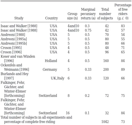
standard model consistent with the data from public good experi-ments? For the one-stage game there are, fortunately, a large number of experimental studies (see Table II). They investigate the contribution behavior of subjects under a wide variety of conditions. In Table II we concentrate on the behavior of subjects in the final period only, since we want to exclude the possibility of repeated games effects. Furthermore, in the final period we have more confidence that the players fully understand the game that is being played.18
The striking fact revealed by Table II is that in the final period of n-person cooperation games (n⬎ 3) without punishment the vast majority of subjects play the equilibrium strategy of complete free riding. If we average over all studies, 73 percent of all subjects choose gi ⫽ 0 in the final period. It is also worth
mentioning that in addition to those subjects who play exactly the equilibrium strategy there are very often a nonnegligible fraction of subjects who play ‘‘close’’ to the equilibrium. In view of the facts presented in Table II, it seems fair to say that the standard model ‘‘approximates’’ the choices of a big majority of subjects rather well. However, if we turn to the public good game with punish-ment, there emerges a radically different picture although the standard model predicts the same outcome as in the one-stage
18. This point is discussed in more detail in Section V. Note that in some of the studies summarized in Table II the group composition was the same for all T periods (partner condition). In others, the group composition randomly changed from period to period (stranger condition). However, in the last period subjects in the partner condition also play a true one-shot public goods game. Therefore, Table II presents the behavior from stranger as well as from partner experiments.
game. Figure II shows the distribution of contributions in the final period of the two-stage game conducted by Fehr and Ga¨chter [1996]. Note that the same subjects generated the distribution in the game without and in the game with punishment. Whereas in the game without punishment most subjects play close to com-plete defection, a strikingly large fraction of roughly 80 percent cooperates fully in the game with punishment.19Fehr and Ga¨chter
19. Subjects in the Fehr and Ga¨chter study participated in both conditions, i.e., in the game with punishment and in the game without punishment. The parameter values for a and n in this experiment are a⫽ 0.4 and n ⫽ 4. It is interesting to note that contributions are significantly higher in the two-stage game already in period 1. Moreover, in the one-stage game cooperation strongly decreases over time, whereas in the two-stage game cooperation quickly converges to the high levels observed in period 10.
TABLE II
PERCENTAGE OFSUBJECTSWHOFREERIDECOMPLETELY IN THEFINALPERIOD OF A
REPEATEDPUBLICGOODGAME
Study Country Group size (n) Marginal pecuniary return (a) Total number of subjects Percentage of free riders (gi⫽ 0)
Isaac and Walker [1988] USA 4and10 0.3 42 83
Isaac and Walker [1988] USA 4and10 0.75 42 57
Andreoni [1988] USA 5 0.5 70 54
Andreoni [1995a] USA 5 0.5 80 55
Andreoni [1995b] USA 5 0.5 80 66
Croson [1995] USA 4 0.5 48 71
Croson [1996] USA 4 0.5 96 65
Keser and van Winden
[1996] Holland 4 0.5 160 84
Ockenfels and
Weimann [1996] Germany 5 0.33 200 89
Burlando and Hey
[1997] UK,Italy 6 0.33 120 66 Falkinger, Fehr, Ga¨chter, and Winter-Ebmer [forthcoming] Switzerland 8 0.2 72 75 Falkinger, Fehr, Ga¨chter, and Winter-Ebmer [forthcoming] Switzerland 16 0.1 32 84
Total number of subjects in all experiments and
report that the vast majority of punishments are imposed by cooperators on the defectors and that lower contribution levels are associated with higher received punishments. Thus, defectors do not gain from free riding because they are being punished.
The behavior in the game with punishment represents an unambiguous rejection of the standard model. This raises the question whether our model is capable of explaining both the evidence of the one-stage public good game and of the public good game with punishment. Consider the one-stage public good game first. The prediction of our model is summarized in the following proposition:
PROPOSITION4.
(a) If a⫹ i⬍ 1 for player i, then it is a dominant strategy for
that player to choose gi⫽ 0.
(b) Let k denote the number of players with a⫹ i⬍ 1, 0 ⱕ
kⱕ n. If k/(n ⫺ 1) ⬎ a/2, then there is a unique equilib-rium with gi⫽ 0 for all i 僆 51, . . . , n6.
(c) If k/(n⫺ 1) ⬍ (a ⫹ j⫺ 1)/(␣j⫹ j) for all players j 僆
51, . . . , n6 with a ⫹ j ⬎ 1, then other equilibria with
positive contribution levels do exist. In these equilibria all k players with a⫹ i ⬍ 1 must choose gi ⫽ 0, while all
other players contribute gj⫽ g 僆 [0,y]. Note further that
(a⫹ j⫺ 1)/(␣j⫹ j)⬍ a/2.
FIGUREII
Distribution of Contributions in the Final Period of the Public Good Game with Punishment (Source: Fehr and Ga¨chter [1996])
The formal proof of Proposition 4 is relegated to the Appendix. To see the basic intuition for the above results, consider a player with a⫹ i ⬍ 1. By spending one dollar on the public good, he
earns a dollars in monetary terms. In addition, he may get a nonpecuinary benefit of at mostidollars from reducing
inequal-ity. Therefore, since a⫹ i ⬍ 1 for this player, it is a dominant
strategy for him to contribute nothing. Part (b) of the proposition says that if the fraction of subjects, for whom gi⫽ 0 is a dominant
strategy, is sufficiently high, there is a unique equilibrium in which nobody contributes. The reason is that if there are only a few players with a⫹ i⬎ 1, they would suffer too much from the
disadvantageous inequality caused by the free riders. The proof of the proposition shows that if a potential contributor knows that the number of free riders, k, is larger than a(n⫺ 1)/2, then he will not contribute either. The last part of the proposition shows that if there are sufficiently many players with a ⫹ i ⬎ 1, they can
sustain cooperation among themselves even if the other players do not contribute. However, this requires that the contributors are not too upset about the disadvantageous inequality toward the free riders. Note that the condition k/(n⫺ 1) ⬍ (a ⫹ j⫺ 1)/
(␣j⫹ j) is less likely to be met as␣jgoes up. To put it differently,
the greater the aversion against being the sucker, the more difficult it is to sustain cooperation in the one-stage game. We will see below that the opposite holds true in the two-stage game.
Note that in almost all experiments considered in Table II, aⱕ 1/2. Thus, if the fraction of players with a ⫹ i⬍ 1 is larger
than 1⁄
4, then there is no equilibrium with positive contribution
levels. This is consistent with the very low contribution levels that have been observed in these experiments. Finally, it is worthwhile mentioning that the prospects for cooperation are weakly increas-ing with the marginal return a.
Consider now the public good game with punishment. To what extent is our model capable of accounting for the very high cooperation in the public good game with punishment? In the context of our model the crucial point is that free riding generates a material payoff advantage relative to those who cooperate. Since c⬍ 1, cooperators can reduce this payoff disadvantage by punish-ing the free riders. Therefore, if those who cooperate are suffi-ciently upset by the inequality to their disadvantage, i.e., if they have sufficiently high ␣’s, then they are willing to punish the defectors even though this is costly to themselves. Thus, the threat to punish free riders may be credible, which may induce
potential defectors to contribute at the first stage of the game. This is made precise in the following proposition.
PROPOSITION5. Suppose that there is a group of n’ ‘‘conditionally
cooperative enforcers,’’ 1ⱕ n’ ⱕ n, with preferences that obey a⫹ iⱖ 1 and
(13) c⬍ ␣i
(n⫺ 1)(1 ⫹ ␣i)⫺ (n8 ⫺ 1)(␣i⫹ i)
for all i僆 51, . . . , n86. whereas all other players do not care about inequality; i.e., ␣i ⫽ i ⫽ 0 for i 僆 5n’ ⫹ 1, . . . , n6. Then the following
strategies, which describe the players’ behavior on and off the equilibrium path, form a subgame perfect equilibrium. ● In the first stage each player contributes gi⫽ g 僆 [0, y].
● If each player does so, there are no punishments in the second stage. If one of the players i 僆 5n’ ⫹ 1, . . . , n6 deviates and chooses gi ⬍ g, then each enforcer j 僆
51, . . . , n’6 chooses pji ⫽ ( g ⫺ gi)/(n’⫺ c) while all other
players do not punish. If one of the ‘‘conditionally coopera-tive enforcers’’ chooses gi⬍ g, or if any player chooses gi⬎
g, or if more than one player deviated from g, then one Nash-equilibrium of the punishment game is being played. Proof. See Appendix.
Proposition 5 shows that full cooperation, as observed in the experiments by Fehr and Ga¨chter [1996], can be sustained as an equilibrium outcome if there is a group of n’ ‘‘conditionally cooperative enforcers.’’ In fact, one such enforcer may be enough (n’⫽ 1) if his preferences satisfy c ⬍ ␣i/(n⫺ 1)(1 ⫹ ␣i) and a ⫹
i ⱖ 1; i.e., if there is one person who is sufficiently concerned
about inequality. To see how the equilibrium works, consider such a ‘‘conditionally cooperative enforcer.’’ For him a⫹ iⱖ 1, so he is
happy to cooperate if all others cooperate as well (this is why he is called ‘‘conditionally cooperative’’). In addition, condition (13) makes sure that he cares sufficiently about inequality to his disadvantage. Thus, he can credibly threaten to punish a defector (this is why he is called ‘‘enforcer’’). Note that condition (13) is less demanding if n’ or ␣i increases. The punishment is constructed
such that the defector gets the same monetary payoff as the enforcers. Since this is less than what a defector would have received if he had chosen gi⫽ g, a deviation is not profitable.
If the conditions of Proposition 5 are met, then there exists a continuum of equilibrium outcomes. This continuum includes the ‘‘good equilibrium’’ with maximum contributions but also the ‘‘bad equilibrium’’ where nobody contributes to the public good. In our view, however, there is a reasonable refinement argument that rules out ‘‘bad’’ equilibria with low contributions. To see this, note that the equilibrium with the highest possible contribution level, gi ⫽ g ⫽ y for all i 僆 51, . . . , n6, is the unique symmetric and
efficient outcome. Since it is symmetric, it yields the same payoff for all players. Hence, this equilibrium is a natural focal point that serves as a coordination device even if the subjects choose their strategies independently.
Comparing Propositions 4 and 5, it is easy to see that the prospects for cooperation are greatly improved if there is an opportunity to punish defectors. Without punishments all players with a⫹ i⬍ 1 will never contribute. Players with a ⫹ i⬎ 1 may
contribute only if they care enough about inequality to their advantage but not too much about disadvantageous inequality. On the other hand, with punishment all players will contribute if there is a (small) group of ‘‘conditionally cooperative enforcers.’’ The more these enforcers care about disadvantageous inequality, the more they are prepared to punish defectors which makes it easier to sustain cooperation. In fact, one person with a suffi-ciently high␣iis already enough to enforce efficient contributions
by all other players.
Before we turn to the next section, we would like to point out an implication of our model for the Prisoner’s Dilemma (PD). Note that the simultaneous PD is just a special case of the public good game without punishment for n ⫽ 2 and gi 僆 50, y6, i ⫽ 1,2.
Therefore, Proposition 4 applies; i.e., cooperation is an equilib-rium if both players meet the condition a⫹ i⬎ 1. Yet, if only one
player meets this condition, defection of both players is the unique equilibrium. In contrast, in a sequentially played PD a purely selfish first mover has an incentive to contribute if he faces a second mover who meets a⫹ i⬎ 1. This is so because the second
mover will respond cooperatively to a cooperative first move while he defects if the first mover defects. Thus, due to the reciprocal behavior of inequity-averse second movers, cooperation rates among first movers in sequentially played PDs are predicted to be higher than cooperation rates in simultaneous PDs. There is fairly strong evidence in favor of this prediction. Watabe, Terai, Haya-shi, and Yamagishi [1996] and HayaHaya-shi, Ostrom, Walker, and
Yamagishi [1998] show that cooperation rates among first movers in sequential PDs are indeed much higher and that reciprocal cooperation of second movers is very frequent.
V. PREDICTIONS ACROSSGAMES
In this section we examine whether the distribution of parameters that is consistent with experimental observations in the ultimatum game is consistent with the experimental evidence from the other games. It is not our aim here to show that our theory is consistent with 100 percent of the individual choices. The objective is rather to offer a first test for whether there is a chance that our theory is consistent with the quantitative evi-dence from different games. Admittedly, this test is rather crude. However, at the end of this section we make a number of predictions that are implied by our model, and we suggest how these predictions can be tested rigorously with some new experiments.
In many of the experiments referred to in this section, the subjects had to play the same game several times either with the same or with varying opponents. Whenever available, we take the data of the final period as the facts to be explained. There are two reasons for this choice. First, it is well-known in experimental economics that in interactive situations one cannot expect the subjects to play an equilibrium in the first period already. Yet, if subjects have the opportunity to repeat their choices and to better understand the strategic interaction, then very often rather stable behavioral patterns, that may differ substantially from first-period-play, emerge. Second, if there is repeated interaction between the same opponents, then there may be repeated games effects that come into play. These effects can be excluded if we look at the last period only.
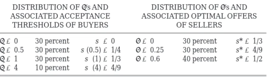
Table III suggests a simple discrete distribution of␣iandi.
We have chosen this distribution because it is consistent with the large experimental evidence we have on the ultimatum game (see Table I above and Roth [1995]). Recall from Proposition 1 that for any given ␣i, there exists an acceptance threshold s8(␣i) ⫽
␣i/(1⫹ 2␣i) such that player i accepts s if and only if sⱖ s8(␣i). In
all experiments there is a fraction of subjects that rejects offers even if they are very close to an equal split. Thus, we (conserva-tively) assume that 10 percent of the subjects have␣ ⫽ 4 which implies an acceptance threshold of s8 ⫽ 4/9 ⫽ 0.444. Another,
typically much larger fraction of the population insists on getting at least one-third of the surplus, which implies a value of␣ which is equal to one. These are at least 30 percent of the population. Note that they are prepared to give up one dollar if this reduces the payoff of their opponent by two dollars. Another, say, 30 percent of the subjects insist on getting at least one-quarter, which implies that␣ ⫽ 0.5. Finally, the remaining 30 percent of the subjects do not care very much about inequality and are happy to accept any positive offer (␣ ⫽ 0).
If a proposer does not know the parameter␣ of his opponent but believes that the probability distribution over␣ is given by Table III, then it is straightforward to compute his optimal offer as a function of his inequality parameter. The optimal offer is given by
(14) s*() ⫽
5
0.5 if i⬎ 0.5
0.4 if 0.235⬍ i⬍ 0.5
0.3 if i⬍ 0.235.
Note that it is never optimal to offer less than one-third of the surplus, even if the proposer is completely selfish. If we look at the actual offers made in the ultimatum game, there are roughly 40 percent of the subjects who suggest an equal split. Another 30 percent offer s僆 [0.4, 0.5), while 30 percent offer less than 0.4. There are hardly any offers below 0.25. This gives us the distribu-tion of in the population described in Table III.
Let us now see whether this distribution of preferences is consistent with the observed behavior in other games. Clearly, we have no problem in explaining the evidence on market games with proposer competition. Any distribution of ␣ and  yields the competitive outcome that is observed by Roth et al. [1991] in all
TABLE III
ASSUMPTIONS ABOUT THEDISTRIBUTION OFPREFERENCES
DISTRIBUTION OF␣’s AND ASSOCIATED ACCEPTANCE
THRESHOLDS OF BUYERS
DISTRIBUTION OF’s AND ASSOCIATED OPTIMAL OFFERS
OF SELLERS
␣ ⫽ 0 30 percent s8 ⫽ 0  ⫽ 0 30 percent s*⫽ 1/3 ␣ ⫽ 0.5 30 percent s8(0.5) ⫽ 1/4  ⫽ 0.25 30 percent s*⫽ 4/9 ␣ ⫽ 1 30 percent s8 (1) ⫽ 1/3  ⫽ 0.6 40 percent s*⫽ 1/2 ␣ ⫽ 4 10 percent s8 (4) ⫽ 4/9
their experiments. Similarly, in the market game with responder competition, we know from Proposition 3 that if there is at least one responder who does not care about disadvantageous inequal-ity (i.e.,␣i⫽ 0), then there is a unique equilibrium outcome with
s⫽ 0. With five responders in the experiments by Gu¨th, March-and, and Rulliere [1997] and with the distribution of types from Table III, the probability that there is at least one such player in each group is given by 1–0.75 ⫽ 83 percent. This is roughly
consistent with the fact that 71 percent of the players accepted an offer of zero, and 9 percent had an acceptance threshold of s8 ⫽ 0.02 in the final period.
Consider now the public good game. We know by Proposition 4 that cooperation can be sustained as an equilibrium outcome only if the number k of players with a⫹ i⬍ 1 obeys k/(n ⫺ 1) ⬍
a/2. Thus, our theory predicts that there is less cooperation the smaller a which is consistent with the empirical evidence of Isaac and Walker [1988] presented in Table II.20In a typical treatment
a⫽ 0.5, and n ⫽ 4. Therefore, if all players believe that there is at least one player with a ⫹ i ⬍ 1, then there is a unique
equilibrium with gi⫽ 0 for all players. Given the distribution of
preferences of Table III, the probability that there are four players with  ⬎ 0.5 is equal to 0.44 ⫽ 2.56 percent. Hence, we should
observe that, on average, almost all individuals fully defect. A similar result holds for most other experiments in Table II. Except for the Isaac and Walker experiments with n⫽ 10 a single player with a ⫹ i ⬍ 1 is sufficient for the violation of the necessary
condition for cooperation, k/(n⫺ 1) ⬍ a/2. Thus, in all these experiments our theory predicts that randomly chosen groups are almost never capable of sustaining cooperation. Table II indicates that this is not quite the case, although 73 percent of individuals indeed choose gi⫽ 0. Thus, it seems fair to say that our model is
consistent with the bulk of individual choices in this game.21
Finally, the most interesting experiment from the perspective of our theory is the public good game with punishment. While in
20. For a⫽ 0.3, the rate of defection is substantially larger than for a ⫽ 0.75. The Isaac and Walker experiments were explicitly designed to test for the effects of variations in a.
21. When judging the accuracy of the model, one should also take into account that there is in general a significant fraction of the subjects that play close to complete free riding in the final round. A combination of our model with the view that human choice is characterized by a fundamental randomness [McKelvey and Palfrey 1995; Anderson, Goeree, and Holt 1997] may explain much of the remaining 25 percent of individual choices. This task, however, is left for future research.