The role of flow regimes for sediment
transport and flooding potential of
river catchments
presented to the Faculty of Science of the University of Neuchˆatel to satisfy the requirements of the degree of Doctor of Philosophy in Science
by
Stefano Basso
Supervisory Committee:
Prof. Dr. Mario Schirmer, Universit´e de Neuchˆatel (Director of the thesis) Prof. Dr. Daniel Hunkeler, Universit´e de Neuchˆatel (Co-director of the thesis) Prof. Dr. Gianluca Botter, Universit`a degli Studi di Padova (Technical supervisor)
Prof. Dr. Peter Molnar, ETH Z¨urich (External reviewer)
Defended: 04.05.2016
Universit´e de Neuchˆatel 2016
Faculté des sciences Secrétariat-décanat de Faculté Rue Emile-Argand 11 2000 Neuchâtel - Suisse Tél: + 41 (0)32 718 2100 E-mail: [email protected]
Imprimatur pour thèse de doctorat www.unine.ch/sciences
IMPRIMATUR POUR THESE DE DOCTORAT
La Faculté des sciences de l'Université de Neuchâtel
autorise l'impression de la présente thèse soutenue par
Monsieur Stefano BASSO
Titre:
“The role of flow regimes for sediment
transport and flooding potential
of river catchments”
sur le rapport des membres du jury composé comme suit:
- Prof. Mario Schirmer, directeur de thèse, Université de Neuchâtel, Suisse
- Prof. Daniel Hunkeler, co-directeur de thèse, Université de Neuchâtel, Suisse
- Prof. Gianluca Botter, Università degli Studi di Padova, Italie
- Prof. Peter Molnar, ETH Zürich, Suisse
Neuchâtel, le 20 mai 2016
Le Doyen, Prof. B. Colbois
SUMMARY
The river flow regime is the main driver of several processes occurring in riverine environments, which are relevant for the sustainable management of water resources. It also determines the sensitivity of the flow distribution itself to a changing climate, and possibly affects catchments’ behaviors with respect to extreme flows. For this reason, understanding links among hydrologic and eco-morphological processes which shape riverine environments is pivotal to ensure safety against flood hazards and the protection of human-valued ecosystem services. In order to reach these goals, quantitative investigations on the links between the flow regime and commonly used metrics in river geomorphology and engineering were pursued in this study.
The variety of the effective discharge for sediment transport observed in different river catch-ments is here related to the underlying heterogeneity of flow regimes. The main climatic and landscape drivers of the effective discharge are identified through an analytic framework, which links the effective ratio (i.e. the ratio between effective discharge and mean streamflow) to the empirical exponent of the sediment rating curve and to the streamflow variability. The anal-ysis shows that different streamflow dynamics intrinsic to erratic and persistent flow regimes (respectively characterized by high and low flow variability) cause the emergence of diverse effec-tive ratios, with larger values associated to erratic regimes. The provided formulation predicts patterns of effective ratios versus streamflow variability observed in a set of catchments of the continental United States, and may support the estimate of effective discharge in rivers belonging to diverse climatic areas.
The capability of a mechanistic analytical model of streamflow distributions to capture statis-tical features of high flows is also investigated. The model builds on a stochastic description of soil moisture dynamics and a simplified hydrologic response, described through different catchment-scale storage-discharge relations. The results show that non-linear relations are needed for a proper characterization of high flows frequencies and to explain the emergence of heavy-tailed streamflow distributions, which is mechanistically linked to the degree of non-linearity of the catchment hydrologic response.
Finally, a novel physically-based analytic expression of the seasonal flood-frequency curve is proposed. The expression is derived from a stochastic model of daily discharge dynamics, whose parameters embody climate and landscape attributes of the contributing catchment and can be estimated from daily rainfall and streamflow data. Only one parameter, which is related to the antecedent wetness condition in the watershed, requires calibration on the observed maxima. Applications in two rivers featured by contrasting daily flow regimes (erratic and persistent) are used to illustrate the potential of the method, which is able to capture diverse shapes of flood-frequency curves emerging in different climatic settings. The model provides reliable estimates of the seasonal maximum flows associated to a set of recurrence intervals, and its performances do not significantly decrease for return times longer than the available sample size. This result is due to the model structure, which allows for an efficient exploitation of the information contained in the entire range of daily flows experienced by rivers. Therefore, the proposed approach may be especially valuable in data scarce regions of the world.
R´ESUM´E
Le r´egime d’´ecoulement de la rivi`ere est le principal moteur de plusieurs processus qui se pro-duisent dans des environnements fluviaux. Ces processus sont importants pour la gestion durable des ressources en eau. Le r´egime d’´ecoulement d´etermine aussi la sensibilit´e de la distribution du flux lui-mˆeme `a une variation climatique, et affecte les comportements des bassins versants dans le cas de flux ´elev´es. Pour cette raison, la compr´ehension des liens entre les processus hy-drologiques et ´eco-morphologiques qui fa¸connent les environnements fluviaux est essentielle pour assurer la s´ecurit´e contre les risques d’inondation et la protection des services ´ecosyst´emiques hu-mains. Afin d’atteindre ces objectifs, il est propos´e ici une ´etude quantitative sur les liens entre le r´egime d’´ecoulement et les m´etriques couramment utilis´ees en g´eomorphologie de la rivi`ere et en ing´enierie.
La vari´et´e de la d´echarge efficace pour le transport des s´ediments observ´es dans diff´erents bassins de rivi`ere est ici li´ee `a l’h´et´erog´en´eit´e sous-jacente des r´egimes d’´ecoulement. Les prin-cipaux ´el´ements climatiques et du paysage responsables de la d´echarge effective sont identifi´es grˆace `a un cadre analytique, qui relie le rapport effectif (i.e. le rapport entre le flux efficace et flux moyen) `a l’exposant empirique des courbes de notation des s´ediments et `a la variabilit´e des flux. L’analyse montre que diff´erentes dynamiques intrins`eques aux flux erratiques et aux flux persistants (caract´eris´ees par la variabilit´e ´elev´ee et faible du flux) provoquent l’´emergence de diff´erentes ratios effectifs, avec des valeurs plus ´elev´ees associ´ees `a des r´egimes de flux erratiques. Le mod`ele pr´edit bien les rapport entre le ratio effectif et la variabilit´e des flux d’un ensemble de bassins des Etats-Unis continentaux, et peut appuyer l’estimation de la d´echarge effective dans des rivi`eres qui appartiennent `a diff´erentes zones climatiques.
La capacit´e d’un mod`ele m´ecanique analytique des distributions des flux `a capturer les pro-pri´et´es des flux ´elev´es est ´egalement ´etudi´ee. Le mod`ele se fonde sur une description stochastique de la dynamique de l’humidit´e du sol, et sur une r´eponse hydrologique simplifi´ee, d´ecrite par des diff´erentes relations de stockage-d´echarge. Les r´esultats montrent que des relations non-lin´eaires sont n´ecessaires pour la caract´erisation correcte des fr´equences des flux ´elev´es et pour expliquer l’´emergence de distributions a queue lourde du flux, ce qui est m´ecaniquement li´e au degr´e de non-lin´earit´e de la r´eponse hydrologique du bassin.
Enfin, une nouvelle expression analytique pour expliquer les courbes inondations-fr´equence saisonni`ere est propos´ee. L’expression est d´eriv´e d’un mod`ele stochastique de la dynamique quotidienne de d´echarge, dont les param`etres repr´esentent les attributs du climat et de paysage du bassin et peuvent ˆetre estim´es `a partir des donn´ees quotidiennes des pr´ecipitations et des flux. Un seul param`etre, qui est li´e `a l’ant´ec´edent ´etat d’humidit´e dans le bassin, n´ecessite une calibration sur les maxima observ´es. Les mod`eles sont appliqu´es dans deux rivi`eres pr´esent´ees en comparant les r´egimes quotidiens d’´ecoulement (erratique et persistante) pour montrer lefficacit´e de la m´ethode, qui est capable de capturer diff´erentes formes de courbes de fr´equence d’inondation ´
flux maximaux saisonniers associ´ees `a un ensemble d’intervalles de r´ecurrence, et les performances du mod`ele ne diminuent pas de mani`ere significative pour des temps de retour plus longs que la taille de l’´echantillon disponible. Ce r´esultat est dˆu `a la structure du mod`ele, qui permet une exploitation efficace de l’information contenue dans l’ensemble des flux quotidiens des rivi`eres. Par cons´equent, l’approche peut ˆetre particuli`erement utile dans les r´egions du monde pour lesquelles les donn´ees sont limit´ees.
Keywords: effective discharge, streamflow variability, river flow regimes, stochastic ana-lytical model, suspended sediment transport, flow dynamics, streamflow distributions, high flows, heavy-tails, ecohydrology, recession analysis, storage-discharge, flood-frequency curves, physically-based, data scarcity.
CONTENTS
Summary . . . . i
List of Figures . . . . viii
List of Tables . . . . xi
1. Introduction . . . . 1
2. Climatic and landscape controls on effective discharge . . . . 5
2.1 Introduction . . . 5
2.2 Observed effective discharge and streamflow variability . . . 6
2.3 An explanatory framework . . . 7
2.4 Conclusions . . . 12
2.5 Supplementary Information . . . 13
2.5.1 Derivation of the analytical expression of the functional-equivalent ratio Rf (eq.(2.3)). . . 13
2.5.2 Derivation of the simplified analytical expressions of the functional-equivalent ratio Rf (eq.(2.4)). . . 14
3. On the emergence of heavy-tailed streamflow distributions . . . . 17
3.1 Introduction . . . 17
3.2 Methods . . . 18
3.2.1 Probabilistic characterization of streamflows . . . 18
3.2.2 Case studies . . . 20
3.2.3 Parameter estimation . . . 20
3.3 Results and Discussion . . . 23
3.4 Conclusions . . . 28
4. A physically-based analytical model of flood-frequency curves . . . . 31
4.1 Introduction . . . 31
4.2 Analytic expression of the seasonal flood-frequency curve . . . 32
4.3 Case studies and parameters estimation . . . 34
4.4 Results . . . 34
4.5 Conclusions . . . 38
4.6 Supplementary Information . . . 39
4.6.1 Derivation of the probability distribution of peak storages, pj(V ) (eq. (4.2)). 39 4.6.2 Derivation of the probability distribution of peakflows, pj(q) (eq. (4.3)). . 41
4.6.3 Uncertainty of the physically-based analytic expression of the seasonal flood-frequency curve . . . 41
Contents
5. Conclusions and Perspectives . . . . 45
5.1 Conclusions . . . 45
5.2 Outlook . . . 46
LIST OF FIGURES
2.1 a) Outlets locations of catchments considered in this study. b) The observed functional-equivalent ratio Rf scales with the coefficient of variation of streamflows
CVq. Solid lines containing most of the observations (shadowed area) represent
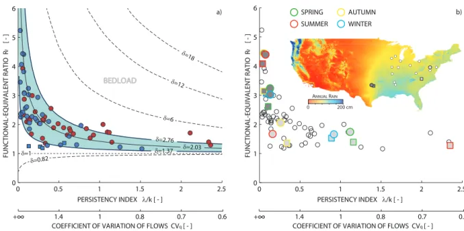
estimate of the analytical model (eq. (2.3)) for δ equal to the 0.1 (δ = 1.37) and 0.9 (δ = 2.76) quantiles of its observed distribution (shown in the inset). . . . 8 2.2 a) Functional-equivalent ratio Rf as a function of the persistency index λ/k. Thick
solid lines represent estimate of the analytical model for δ equal to the 0.1 (δ = 1.37) and 0.9 (δ = 2.76) quantiles of its observed distribution, and contain most of the observations (shadowed area), which refer to suspended sediment transport. Blue squares are cases with δ ∼ 1 (δ < 1.20). Blue dots tag catchments with observed δ lower than the mean value (δ < 2.03), while basins with δ > 2.03 are marked by red dots. The analytical estimate for the discriminating δ value is represented with a thin solid line. Analytical estimates for other values of δ usually associated to bed or dissolved loads are also displayed with dotted lines. b) Clustering of Rf values of catchments belonging to different climatic areas. Dark
gray dots and squares represent basins in South-Central US (respectively Elm Fork and Little Elm Creek in Texas), while light gray dots and squares tag catchments in Eastern US (respectively Conococheague Creek in Maryland and South Yadkin River in North Carolina). Locations of their outlets are displayed in the map, which also shows total annual rainfall throughout the United States. Green, red, yellow and blue contours of markers respectively indicate spring, summer, autumn and winter seasons. . . 10
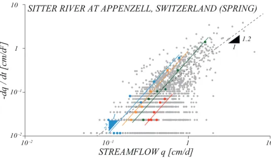
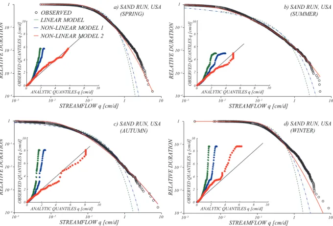
3.1 Flow recession analysis for the Sitter River at Appenzell in the spring season. Grey dots represent the cloud of points obtained by plotting flow q versus time derivative of the flow −dq/dt for decreasing branches of the hydrograph. Colored points and lines display four individual recessions and their regression lines. Notice that regression lines of individual recessions are parallel and shifted, and exhibit steeper slopes than the regression line of the ensemble of points (dotted black line). 23 3.2 Flow duration curves for the Sand Run (WV) catchment during spring (a), summer
(b), autumn (c) and winter (d) seasons. Plots are on a log-log scale. Dots represent duration curves estimated from observed data series. Green dotted lines illustrate results of the linear model, while estimates of the non-linear model are represented with dashed-dotted blue lines (NL1) and solid red lines (NL2). Insets show q-q plots for the case studies. . . 24
List of Figures
3.3 Flow duration curves for (a) the Sitter river at Appenzell and (b) the Thur river at Andelfingen (Switzerland) during the spring season. Plots are on a log-log scale. Dots represent duration curves estimated from observed data series. Green dotted lines illustrate results of the linear model, while estimates of the non-linear model are represented with dashed-dotted blue lines (NL1) and solid red lines (NL2). Insets show q-q plots for the case studies. . . 24
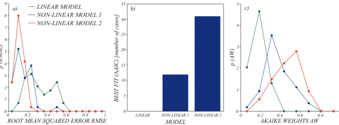
3.4 Indices summarizing the goodness of fit of the alternative models with respect to observed data. (a) Probability distribution of the Root Mean Squared Error (RMSE) between modeled and observed flow cdfs; (b) Number of cases each model gives the best performance, measured by using Akaike Differences (∆AIC); (c) Probability distribution of the Akaike Weights (AW ) assigned to each model. In (a) and (c) green lines display the performance of model L, while blue and red lines the performance of models NL1 and NL2. . . . 26
3.5 (a) Flow duration curve for the Rio Tanama (PR) catchment during the winter season. Plots are on a log-log scale. Dots represent the duration curve estimated from the observed data series. The dotted red line displays the estimate of model NL2 when a fixed K is used. The solid red line instead shows the estimate of model NL2 when the observed correlation between qpand K (b) is numerically accounted
for in the model. For this purpose, the numerical counterpart of the analytical model has been run by selecting a different value of K from the regression (dotted line in Figure 5b) for each runoff event. . . 28
4.1 Excess storage V and streamflow q dynamics as produced by the mechanistic-stochastic model used in this study [Botter et al., 2009]. Flows (excess storages) occurring immediately after increments are termed peakflows (peak storages) and labeled with grey dots. . . 33
4.2 Seasonal flood-frequency curves for the Sand Run (West Virginia) and the Big Eau Plein River (Wisconsin). Curves obtained from the entire series of observed data through Weibull plotting position are represented with dots, while solid red lines display estimates of the proposed analytical model. Confidence intervals of the model estimates are plotted with dotted red lines. . . 35
4.3 Normalized flood frequency curves (i.e., seasonal maximum divided by the average daily flow, < q >) in four case studies characterized by decreasing persistency index ϕ. For the calculation of the persistency index, K has been estimated as in Basso et al. [2015a]. Values of the coefficient of variation of daily flows associated to the four case studies are 1.30 (blue), 2.22 (green), 2.95 (yellow) and 4.13 (red). A decrease of the persistency index associated to the daily flow regime results in lower magnitude of events characterized by short return periods and higher magnitude of rare events in erratic regimes. . . 36
List of Figures
4.4 a,b) Performance of the proposed analytical model in predicting flood-frequency curves with short data series. Samples of seasonal data (20, 10 or 5 years) selected from the entire dataset through a moving window are used to estimate analytic seasonal flood-frequency curves. Model results are then compared with the esti-mate obtained from the complete data series through Weibull plotting position. Errors are computed for a set of return periods (from 10 to 60 years). The plot shows the fraction of cases displaying an error (ϵ) lower than 25%. The shorter the number of years (seasons) of available data, the lower the fraction of cases displaying ϵ < 25%. The results seem instead quite constant for increasing return periods. The same behavior is found by setting different thresholds for the ac-ceptable error. c,d) Comparison between performances of the proposed analytical model and of generalized extreme value (GEV) distributions calibrated through maximum likelihood on the same samples. Performances are comparable for long data series available (e.g., 20 years) and short return periods (e.g., 10 years). The proposed method exhibits better performances for rare events (high return peri-ods), particularly when only short observed data series (e.g., 5 years) are available to constrain the models. . . 37
LIST OF TABLES
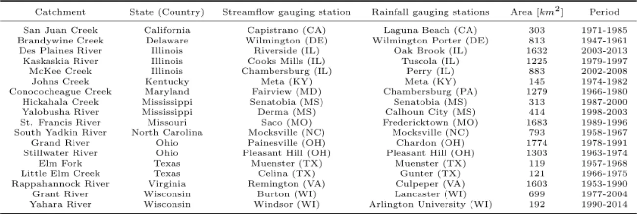
S2.1 Summary information about the catchments used in this study. . . 14 S2.2 Seasonal features of the analyzed catchments: average streamflow < q >,
coeffi-cient of variation of flows CVq, exponent δ and coefficient β of the sediment rating
curve, mean grain size d50 of sediments transported in suspension. d50 has been
calculated for each catchment and season as the median value among limited field measurements available. . . 15
3.1 Summary information about the catchments used in this study. . . 21 3.2 Estimates of mean rainfall frequency (λP), mean frequency of effective rainfall (λ),
mean rainfall depth (α), recession rate (k, linear model), recession exponent (a) and coefficient K (non-linear model) for the study catchments. . . . 22 3.3 Goodness of fit of linear (L) and non-linear (NL1 and NL2) models. The
ta-ble reports the mean values, obtained by averaging the results of the application of models to all the considered catchments and seasons, of Nash-Sutcliffe Co-efficient (NSC), Root Mean Square Error (RMSE), rescaled Akaike Information Criterion (AICc), Akaike Differences (∆AIC) and Akaike Weight (AW ). NSC =
1 −
∑u
f =1(ˆqf−qf)2
∑u
f =1(qf−u1∑uf =1qf)
2, where f is the index of u = 100 log-spaced values of cumulated probability selected in the range 10−4− 1, and q and ˆq the correspond-ing observed and analytic flow values (quantiles). RMSE = √RSS/n, where RSS =∑ni=1(log Di− log ˆDi)2 is the residual sum of squares, and Di and ˆDi are
observed and analytic estimates of duration of a series of n flow values (sample size). AICc = 2(g+1)n + ln(RSS/n) + 2g(g+1)n−g−1, where g is the number of
param-eters of each model. ∆AIC = AICc,m − AICc,min, where AICc,min is the
mini-mum value of AICc among those obtained for the r different models (m ∈ [1, r]).
AW = ∑ exp(−∆AICm/2) r
m=1exp(−∆AICm/2). . . 26
S4.1 Estimates of mean rainfall depth (α[cm]), frequency of effective rainfall (λ[d−1]), recession exponent (a[−]) and coefficient (K[cm1−a/d2−a]) for the study catchments. 44
1. INTRODUCTION
The heavy hydrological modifications faced by rivers during the 20th century in many regions of the world, especially due to damming and intense human exploitation of water resources, triggered interest in understanding the influence of streamflow fluctuations on riverine environments and their capability to provide human-valued ecosystem services.
Poff et al. [1997], by introducing the paradigm of natural flow regime, offered a benchmark to assess the dynamic state of rivers and acknowledged the driving role of flow dynamics for ecological and morphological processes. The control exerted by the flow regime on e.g. availability of habitats for biological species, riparian vegetation growth, transport of solutes and sediments, inundation dynamics of river floodplains and hydropower production is mediated by physical, chemical and biological variables (e.g. water depth and velocity, temperature, turbidity, oxygen content) which influence the concerned processes.
In order to provide a quantitative description of the streamflow dynamics associated to distinct flow regimes, lists of relevant hydrologic metrics have been compiled [Richter et al., 1996]. These metrics are usually derived from data series or distributed physically-based models of catchments, whose parameters are calibrated in order to reproduce the observed hydrograph. Distributed models perform well for the study and prediction of punctual events, such as the erosion of specific river reaches. However, their intense data and time requirements make them less suited when large scale patterns and river management issues are investigated, or for comparing the driving role of flow regimes for processes encompassing different fields (e.g. geomorphology and ecology) and several case studies.
In these cases, a quantitative description of the flow regime through the probability distri-bution of streamflows provides an alternative framework, where ecological and morphological features can be directly linked to the underlying streamflows and the effect of their overall vari-ability can be assessed using a derived distribution approach. Examples of this approach are represented by the works of Vogel and Fennessey [1995], Camporeale and Ridolfi [2006] and Doyle and Shields [2008].
Also the characterization of flooding by rivers has been traditionally based on high dimen-sional models (e.g., for predicting timing and peak values of high flows) or statistical methods (e.g. Castellarin et al. [2012]), which profit from the available observations of extreme events to estimate frequency and magnitude of high flows, disregarding their links to the underlying hydrologic regime. These approaches proved successful, and allowed for large improvements in the evaluation of hazard posed by flooding to lives and properties.
However, natural and human-induced changes of the driving processes (e.g. precipitation and streamflow generation) [Milly et al., 2005] and data scarcity intrinsic to most regions of the world demand for an efficient exploitation of all available information, included those provided by intermediate and low flows. Indeed, the flow regime may contain signatures of the flooding
Chapter 1. Introduction
potential of a river, and provide precious information that can be used to lower the related risk. First steps in this direction have been made by Sivapalan et al. [2005] and Guo et al. [2014], who investigated the relation between catchment water balance and flooding behavior through experimental and modeling approaches.
Recently, Botter et al. [2007a] proposed a lumped mechanistic-stochastic model of daily flow dynamics, which provides an analytic expression of the probability distribution of streamflows in terms of climatic and landscape attributes of the contributing basin. The framework applies to rain-fed catchments during seasonal time frames, and allows for a classification of river flow regimes based on the underlying daily flow variability. Erratic and persistent regimes are iden-tified, respectively characterized by high and low flow variability. The approach builds on a catchment-scale balance of the soil moisture in the root zone, driven by stochastic increments due to infiltration from rainfall and losses due to evapotranspiration and events of instantaneous release of the water exceeding a certain soil moisture threshold (i.e. the water holding capacity of the soil). These events constitute the effective rainfall and recharge the hydrologic storage of the catchment. From here the water is released to the river according to a deterministic storage-discharge relation, which can be either linear or non-linear.
The introduction of this framework, which is especially suited to investigate similarity and dif-ferences among rivers and to identify general behaviors associated to distinct hydrologic regimes, fostered studies on the role of the flow regime as driver of e.g. riparian vegetation dynamics [Doulatyari et al., 2015], hydropower production [Basso and Botter, 2012; Lazzaro et al., 2013] and grazing by benthic organisms [Ceola et al., 2013]. The set of riverine natural processes stud-ied within this framework is further expanded in the work illustrated in the following, where issues related to river geomorphology (namely the estimation of the effective discharge) and flooding potential of catchments are investigated.
Aims and objectives
The general goal of this work is to provide a deeper understanding of the driving role of climatic and morphologic attributes of river catchments for a set of riverine processes ranging from sedi-ment transport to flooding potential. The focus is on commonly used metrics and tools applied in practice, as the effective discharge and the flood-frequency curve. This objective is pursued through the novel development of stochastic physically-based analytical tools, which are then tested against observational data. These approaches are especially designed to deal with data scarcity, in order to allow for their widespread application also in sparsely gauged regions of the world.
The specific research objectives of this work are:
• advancing the capability of an existing stochastic model of streamflow to characterize high flows and tails of flow distributions;
• deriving physically-based analytic models to estimate effective discharge and flood-frequency curves in catchments belonging to different climatic regions;
• investigating the capability of the selected classification of flow regimes to unravel the observed varieties of the effective discharge and the flood-frequency curve;
Chapter 1. Introduction
• disentangling climatic and landscape controls on sediment transport and flooding behaviors in river catchments;
Particular attention is devoted to the development of tools suited to be applied in context char-acterized by data scarcity.
The achievement of these goals constitutes an essential step to study the role of high flows in river ecosystems and develop robust approaches providing a quantitative characterization of riverine dynamics.
Thesis structure
Results of the outlined research are presented in this manuscript as follows:
Chapter 2 discusses the causes of the observed heterogeneity of the effective discharge for sediment transport. An analytic framework is introduced, which links the effective discharge to river flow variability and the underlying climatic and landscape controls. The effects of distinct streamflow dynamics typical of erratic and persistent regimes are identified, and results checked through data gathered in 18 case studies.
Chapter 3 investigates the capability of a mechanistic stochastic model of flow duration curves to resemble statistical properties of high flows. 16 catchments are used as case studies. Different relations between catchment water storage and discharge, and alternative parameter estimation methods are evaluated. Conditions leading to the emergence of heavy-tailed streamflow distri-butions are also identified, and their implications for high flows characterization debated.
Chapter 4 presents a novel physically-based analytical model of flood-frequency curves. The analytical derivation of the extremal distribution of streamflows is described, and outcomes of the established link between daily flow dynamics and hydrologic extremes are discussed through a set of applications in two catchments. The link between flow regime and shape of the flood-frequency curve and the model performance in data scarce contexts are especially discussed.
Chapter 5 summarizes pivotal findings and conclusions. Future challenges and research per-spectives on these topics are also delineated.
2. CLIMATIC AND LANDSCAPE CONTROLS ON EFFECTIVE DISCHARGE
Basso, S.123, A. Frascati4, M. Marani35, M. Schirmer12, G. Botter5 (2015), Climatic and landscape controls on effective discharge, Geophys. Res. Lett., 42, 84418447,
doi:10.1002/2015GL066014.
Abstract
The effective discharge constitutes a key concept in river science and engineering. Notwith-standing many years of studies, a full underNotwith-standing of the effective discharge determinants is still challenged by the variety of values identified for different river catchments. The present paper relates the observed diversity of effective discharge to the underlying heterogeneity of flow regimes. An analytic framework is proposed, which links the effective ratio (i.e. the ratio between effective discharge and mean streamflow) to the empirical exponent of the sediment rating curve and to the streamflow variability, as resulting from climatic and landscape drivers. The analytic formulation predicts patterns of effective ratio versus streamflow variability observed in a set of catchments of the continental United States, and helps in disentangling the major climatic and landscape drivers of sediment transport in rivers. The findings highlight larger effective ratios of erratic hydrologic regimes (characterized by high flow variability) compared to those exhibited by persistent regimes, which are attributable to intrinsically different streamflow dynamics. The framework provides support for the estimate of effective discharge in rivers belonging to diverse climatic areas.
2.1 Introduction
The concept of dominant or channel-forming discharge is central to geomorphological sciences, river engineering and restoration practices. Described as the discharge which shapes the cross section of natural rivers or transports the most sediments over long time periods, the dominant flow is used in the design of stable morphological configuration of channels [Shields et al., 2003; Doyle et al., 2007] and to estimate sedimentation rate and lifespan of reservoirs [Podolak and Doyle, 2015]. Moreover, dominant flows summarize the hydrologic forcing in models studying long-term evolution of rivers (see e.g. Frascati and Lanzoni [2009]) and the related incision patterns (see Lague et al. [2005] and references therein).
1
Department of Water Resources and Drinking Water, Eawag - Swiss Federal Institute of Aquatic Science and Technology, D¨ubendorf, Switzerland.
2
Centre for Hydrogeology and Geothermics (CHYN), University of Neuchˆatel, Neuchˆatel, Switzerland.
3Department EOS, Duke University, Durham, NC, USA. 4
Shell Global Solutions International, Rijswijk, The Netherlands.
Chapter 2. Climatic and landscape controls on effective discharge
Several methods have been proposed in the literature to estimate the magnitude of the channel-forming discharge. In some cases, the dominant flow is identified with the bankfull discharge, evaluated from field surveys as the break point between main channel and floodplain [Andrews, 1980]. Other studies suggest equivalence between the channel-forming discharge and flows char-acterized by suitable return times (e.g. 1.5 years) [Simon et al., 2004]. In order to address the role of both morphological and hydrological factors, Wolman and Miller [1960] proposed to estimate the dominant flow by combining information contained in the frequency distribution of streamflows and the sediment rating curve, giving rise to the concept of effective discharge. Thereafter, empirical, theoretical and numerical studies on effective discharge flourished in the literature, providing sometimes contrasting results (see e.g. Bunte et al. [2014]). Effective dis-charge was found to vary significantly among catchments as a function of climate and sediment rating characteristics, which encapsulate differences of morphology, bed sediment composition, hydrodynamic conditions and, as a consequence, between dominant transport mechanisms (i.e. suspended versus bedload) [Emmett and Wolman, 2001; Simon et al., 2004]. Previous investi-gations (e.g. Vogel et al. [2003]; Goodwin [2004]; Doyle and Shields [2008]; Quader and Guo [2009]) also suggest the effective discharge to be significantly affected by the variability of river flows. For example, Bolla Pittaluga et al. [2014] showed that fluctuations of the hydrodynamic forcing implied by hydrologic variability do not prevent rivers from achieving a quasi-equilibrium morphodynamic state linked to a steady effective forcing, which differs however from typical channel-forming estimates (e.g. the bankfull discharge). Notwithstanding many years of studies, a consistent framework that enables separating hydrologic and landscape controls on the effective discharge and explains the observed patterns of sediment delivery across a gradient of climatic and landscape conditions is still lacking.
In this work, a framework is presented which links the effective discharge to the degree of non-linearity of the sediment rating curve and to streamflow variability, as resulting from climatic and landscape drivers. The framework builds on a physically-based stochastic representation of streamflow dynamics and a lumped description of the sediment transport capacity, and is tested using suspended sediment data observed in a set of catchments in the continental United States. The proposed framework gives insight into the major climatic and morphologic controls of sediment transport in rivers.
2.2 Observed effective discharge and streamflow variability
In this paper, the effective discharge is defined as the constant water flow rate resulting in the same long-term sediment load generated by the complete frequency distribution of streamflows. Doyle and Shields [2008] termed it functional-equivalent discharge qf, to distinguish it from
alternate definitions proposed in the literature (e.g. Wolman and Miller [1960] and Vogel et al. [2003]). Mathematically, the functional-equivalent discharge qf is defined as:
∫ +∞ 0
qsps(qs)dqs= β qf
δ (2.1)
where qs is a stochastic variable representing the flow of sediments at-a-station and ps(qs) its
probability density function. The empirical coefficients δ and β describe the instantaneous power law relation between water and sediment flows, qs = βqδ (hereafter termed sediment rating
curve), whose physical interpretation has been the goal of extensive research (e.g. Syvitski et al. [2000]). The validity of such a relation is a basic assumption of this work. Therefore, cases
Chapter 2. Climatic and landscape controls on effective discharge
where the power law relation between water and sediment flows may be significantly distorted (e.g. supply-limited catchments, rivers with extensive floodplains or strongly varying sediment storage) are not considered.
In order to introduce dimensionless quantities, we define the functional-equivalent ratio (Rf)
as: Rf = qf < q > = [ 1 β ∫+∞ 0 qsps(qs)dqs ]1 δ < q > (2.2)
Rf scales the functional-equivalent discharge qf by the average discharge < q > (see also Tucker
and Bras [2000]), which is a common statistic of river flows, relatively simple to estimate also in poorly gauged regions based on climatic data (e.g. Hrachowitz et al. [2013]). Since the sediment flow qs is a non-linear function of q, its probability density function, ps(qs) (right-hand side of
eq. (2.2)), should strongly depend on the underlying streamflow distribution. As a consequence, the streamflow variability constitutes a major driver of Rf. The effective ratio can be profitably
used to infer long-term (e.g. annual or decadal) sediment transport rates from instantaneous load-discharge relations, correctly accounting for the actual range of streamflows experienced by rivers.
The relation between Rf and streamflow variability is here analyzed by using a data set of
18 catchments in the continental US (Figure 2.1a), for which synchronous data of water and suspended sediment flows were available (summary information for the case studies are reported in Supporting Information, Tables S2.1 and S2.2). Morphological and climatic attributes of the catchments are diverse, ranging from the semi-arid South-Central to the humid Eastern US, and spanning rugged mountainous terrains, gently rolling hills and flatter plains. The land cover is primarily agricultural and forest, with some catchments including urbanized areas. The analyzed rivers are not impacted by significant flow regulation. In some cases, river reaches have undergone straightening and channelization, and topsoil or bank and streambed erosion is a known issue. The mean grain size of sediments transported in suspension (d50) ranges from less than 0.001 to
0.029 mm.
Figure 2.1b displays (white dots) observed Rf as a function of the coefficient of variation of
streamflows, CVq (defined as the ratio between standard deviation and mean of the observed
flows), for every seasons of the considered case studies. Despite some scattering, a clear pattern emerges from the plot shown in Figure 2.1b: low values of the functional-equivalent ratio are associated to low CVq, whereas Rf increases significantly for increasing values of the coefficient
of variation of flows. Accordingly, the functional-equivalent discharge qf is only slightly larger
than the average discharge for rivers exhibiting weak variability of flows, whereas it increases (up to 5 times the average flow) for rivers characterized by pronounced streamflow variability.
2.3 An explanatory framework
The observed variations of the functional-equivalent ratio as a function of streamflow variability are explained by adopting a lumped framework recently proposed by Botter et al. [2013] to characterize and classify flow regimes. According to this framework, the variability of river flows results from the interplay between the frequency of effective (i.e. streamflow-producing) rainfall events (λ) and the mean catchment response time (1/k). Censoring of rainfall events by soil moisture deficit controls the value of λ, which is bounded from above by the rainfall
Chapter 2. Climatic and landscape controls on effective discharge ! ( ! ( !( ! ( ! ( ! ( ! ( ! ( ! ( ! ( ! ( ! ( ! ( ! ( ! ( ! ( ! ( ! ( a) USA ATLANTIC OCEAN PACIFIC OCEAN 10 1 1 5 3 . 0 2 3 4 5
COEFFICIENT OF VARIATION OF FLOWS CVq
FUNCTIONAL-EQUIVALENT RATIO Rf 1 2 3 0 10 20 30 # OF CASES δ δ = 1 .37 δ= 2.7 6 4 VALUE OF 0 b) 6
Fig. 2.1: a) Outlets locations of catchments considered in this study. b) The observed functional-equivalent
ratio Rf scales with the coefficient of variation of streamflows CVq. Solid lines containing most
of the observations (shadowed area) represent estimate of the analytical model (eq. (2.3)) for δ equal to the 0.1 (δ = 1.37) and 0.9 (δ = 2.76) quantiles of its observed distribution (shown in the inset).
Chapter 2. Climatic and landscape controls on effective discharge
frequency and chiefly depends on catchment-scale evapotranspiration rates (in turn determined by vegetation cover and climate). The parameter k expresses the flow decay rate when recessions are assumed exponential, and its value embeds catchment-scale morphological and hydrological features, like the mean length of hydrologic pathways and soil conductivity [Botter et al., 2007b]. When the mean interarrival time of flow-producing rainfall events is shorter than the mean catchment response time (λ > k), the river is continually fed by pulses delivered from the contributing catchment, and the range of streamflows observed between pulses is reduced. River flows are weakly variable around the mean, and the arising flow regime is termed persistent. When λ < k, effective rainfall events are interspersed in between long periods of flow recession, and a wider range of streamflows is observed. In this case an erratic regime emerges, characterized by high flow variability. The ratio λ/k (termed persistency index) fully determines the coefficient of variation of streamflows, since CVq=
√
k/λ in this framework (see Supporting Information). Coupling the analytical expression for the probability distribution of streamflows derived by Botter et al. [2007a] (see Supporting Information) and the sediment rating curve qs = β qδ,
analytical expressions for the probability distribution of sediment flows, ps(qs), and its statistical
moments can be derived (eqs.(S2.4) and (S2.5) in Supporting Information). The integral in eq.(2.2) can thus be expressed as a function of climate and landscape attributes of the catchment. Accordingly, the functional-equivalent ratio Rf can be expressed as:
Rf = k λ [ Γ(λk+ δ) Γ(λk) ]1 δ = CVq2 [ Γ(CVq−2+ δ) Γ(CVq−2 ) ]1 δ (2.3)
Notice that the functional-equivalent ratio only depends on the persistency index λ/k (or, alter-natively, on the coefficient of variation of streamflows) and on the exponent δ of the sediment rating curve. The ratio λ/k embeds the effects of rainfall variability and soil drainage, whereas δ summarizes sediments size (i.e. suspended or bedload transport), erodibility of hillslopes and local conditions of river bed (e.g. armoring) [Bunte et al., 2014].
When δ is integer, eq.(2.3) can be written in a simpler way:
Rf = 1 if δ = 1 √ 1 +kλ if δ = 2 3 √( 1 +kλ) (1 + 2kλ) if δ = 3 (2.4)
Eq. (2.4) clarifies that when the catchment hydrologic response is flashy (high k), the rainfall frequency is low or the soil water deficit in the root zone is pronounced (i.e. low λ, as it might happen in semi-arid climates) the value of Rf increases (i.e. the functional-equivalent discharge
is larger than the mean). However, the sensitivity to λ/k is modulated by the value of δ, as discussed later.
In Figure 2.1b, the analytical expression for Rf (eq. (2.3)) is plotted as a function of CVq, by
assuming δ equal to the 0.1 (δ = 1.37) and 0.9 (δ = 2.76) quantiles of its empirical distribution across the case studies (shown in the inset). The analytical curves (contours of the shadowed area) contain most of the observations, thereby suggesting that the proposed model is able to capture the first-order controls on the effective discharge.
Figure 2.2a displays (continuous lines) theoretical patterns of the functional-equivalent ratio Rf as a function of the persistency index, for different values of δ. Rf tends to one for very
Chapter 2. Climatic and landscape controls on effective discharge BEDLOAD ! ! ! ! ! ! ! ! ! ! ! ! ! ! ! ! ! ! 0 0.5 1 1.5 2 2.5 0 1 2 3 4 5 6 δ=2.76 δ=1.37 δ=18
COEFFICIENT OF VARIATION OF FLOWS CVq [ - ]
+∞ 1.4 0.8 0.7 FUNCTIO NAL-EQUIVAL ENT RATIO R f [ - ] δ=1 δ=0.82 δ=6 δ=12 δ=2.03 1 0.6 0 0.5 1 1.5 2 2.5 0 1 2 3 4 5 6 FUNCTIO NAL-EQUIVAL ENT RATIO R f [ - ]
COEFFICIENT OF VARIATION OF FLOWS CVq [ - ] PERSISTENCY INDEX λ/k [ - ] +∞ 1.4 1 0.8 0.7 0.6 SPRING SUMMER AUTUMN WINTER a) b) 0 200 cm ANNUAL RAIN PERSISTENCY INDEX λ/k [ - ]
Fig. 2.2: a) Functional-equivalent ratio Rf as a function of the persistency index λ/k. Thick solid lines
represent estimate of the analytical model for δ equal to the 0.1 (δ = 1.37) and 0.9 (δ = 2.76) quantiles of its observed distribution, and contain most of the observations (shadowed area), which refer to suspended sediment transport. Blue squares are cases with δ ∼ 1 (δ < 1.20). Blue dots tag catchments with observed δ lower than the mean value (δ < 2.03), while basins with δ > 2.03 are marked by red dots. The analytical estimate for the discriminating δ value is represented with a thin solid line. Analytical estimates for other values of δ usually associated to bed or dissolved loads are also displayed with dotted lines. b) Clustering of Rf values of
catchments belonging to different climatic areas. Dark gray dots and squares represent basins in South-Central US (respectively Elm Fork and Little Elm Creek in Texas), while light gray dots and squares tag catchments in Eastern US (respectively Conococheague Creek in Maryland and South Yadkin River in North Carolina). Locations of their outlets are displayed in the map, which also shows total annual rainfall throughout the United States. Green, red, yellow and blue contours of markers respectively indicate spring, summer, autumn and winter seasons.
Chapter 2. Climatic and landscape controls on effective discharge
stable (persistent) regimes, and significantly increases for low values of the persistency index (i.e. high values of CVq characteristic of erratic flow regimes), approaching infinity for extremely
variable flows (λ/k 7→ 0). The higher the exponent of the sediment rating curve the higher the effective ratio and the smoother its increment with decreasing λ/k (increasing flow variability). High values of δ (δ > 3, see Figure 2.2a) are typically associated to bedload transport [Emmett and Wolman, 2001], and correspond to highly non-linear sediment rating curves which mimic the effect of a minimum threshold of movement. Interestingly, Bunte et al. [2014] and Lanzoni et al. [2015] suggested that the effective discharge for gravel transport should correspond to the maximum observed discharge, which implies Rf >> 1 (in agreement with the theoretical
analysis presented here). On the other hand, δ < 1 causes a decrease of the functional-equivalent ratio with increased flow variability. Values of δ smaller than one are uncommon in sediment transport [Sholtes et al., 2014], but may be appropriate for characterizing the flushing of geogenic and anthropogenic solutes [Neal et al., 2012], where in fact upscaled load-discharge relations need to be suitably adjusted to account for hydrologic variability (e.g. Basu et al. [2010]).
Values of δ in the catchments analyzed in this study well represent the range of values reported in the literature for suspended sediment flows (δ ∈ [1, 3]) [Nash, 1994]. Case studies displaying δ ∼ 1 (δ < 1.20, tagged with squares in Figure 2.2a) lay near the corresponding analytical curve (Rf = 1) and thus confirm that in these circumstances the functional-equivalent discharge is
almost insensitive to flow variability, being qf ∼< q > regardless of the type of flow regime.
Colored dots in Figure 2.2a represent observed Rf versus CVq−2 = λ/k for the same set of
catchments shown in Figure 2.1. Most of the observations fall within the range predicted by the analytical model (shadowed area in Figure 2.2a). Case studies exhibiting δ lower than the average observed value (δ < 2.03) are tagged with blue dots, while red dots correspond to cases with δ > 2.03. Though considerable scatter appears for high flow variability (left side of the plot), the stratification of the two groups of observations seems to support the layering predicted by the model for different exponents of the sediment rating curve, with larger values of Rf associated
to larger values of δ.
The existence of distinct values of the functional-equivalent ratio for erratic (CVq > 1.1, 59
cases) and persistent (CVq < 0.9, 6 cases) regimes has been quantitatively checked by means
of statistical hypothesis testing. Intermediate regimes (0.9 < CVq < 1.1) have been excluded
from the analysis, in agreement with Botter et al. [2013]. The null hypothesis that observed Rf values in persistent and erratic regimes are sampled from distributions with equal medians
has been tested through the Wilcoxon rank sum test. The null hypothesis was rejected at the 5% significance level, thereby implying that the median functional-equivalent ratios of erratic and persistent rivers are statistically different. Because of the different size of the two samples (erratic and persistent regimes), the test has been repeated by dividing cases with CVq lower or
higher than the observed median value across the catchments/seasons considered (CVq= 1.92),
with analogous results.
Distinct streamflow dynamics exhibited by erratic and persistent regimes are the physical driver of the different behaviors of these systems. When flows weakly vary around their mean value (persistent regimes), the probability of high flows and even higher magnitudes of sediment transport (implied by non-linearity of the sediment rating curve) is very low. The magnitude of such events is overshadowed by the corresponding low probability of occurrence, and high flows weakly contribute to long-term sediment transport. Erratic regimes, instead, are composed of a sequence of high flows interspersed in between prolonged periods of low flows (i.e. droughts), which may not be effective in mobilizing sediments (e.g. the shear stress they exercise is under
Chapter 2. Climatic and landscape controls on effective discharge
the threshold of movement). As a result, only high flows are responsible for sediment transport, and the functional-equivalent discharge increases significantly.
Spatial patterns of river flow regimes are the complex by-product of large scale climatic drivers and local heterogeneities (e.g. soil, vegetation, geology). Nevertheless, when climatic attributes like seasonal rainfall and potential evapotranspiration are the primary controls on streamflow variability [Botter et al., 2013], functional-equivalent ratios of rivers could mirror the underlying climatic patterns. An example of climatic clustering is shown in Figure 2.2b, which highlights Rf
values of two groups of catchments subject to very diverse climatic conditions (map shows total annual precipitation). Light gray dots tag basins in Eastern US (Maryland and North Carolina), while dark gray dots indicate South-Central catchments (Texas). Because of their semi-arid climate, Texas catchments are characterized by extremely erratic flow regimes throughout the year, and are located in the left-upper part of the plot. For these rivers qf is several times larger
than the mean streamflow in all cases. Rf is instead less than 2 in every season for rivers of the
Eastern Coast of US (right-lower part of the plot in Figure 2.2b), because of the more frequent rainfall input, which leads the seasonal regime to shift from persistent to slightly erratic.
These results, jointly with recent advances in the prediction of flow regimes using climatic and morphologic data [Doulatyari et al., 2015], support the possibility of applying the present framework for first-order estimates of functional equivalent discharge in rivers belonging to dif-ferent geographic and climatic areas, based on rainfall and landscape attributes. This represents the goal of ongoing research.
2.4 Conclusions
The diversity of effective discharges observed in rivers is here explained in terms of the underlying heterogeneity of flow regimes. The ratio between effective discharge and mean streamflow (effec-tive ratio) is analytically expressed as a function of the exponent of the sediment rating curve and the coefficient of variation of daily flows, which in turn depends on streamflow-producing rainfall frequency and mean catchment response time. The analytic expression captures the first-order controls on the effective ratio for suspended sediment in a set of 18 case studies in the continental US. High values of the effective ratio are associated to larger exponents of the sediment rating curve and to more erratic flow regimes (high flow variability). Instead, the effective discharge is only slightly higher than the average flow in persistent regimes (weak flow variability). This is the by-product of distinct streamflow dynamics, which cause high flows to be the main responsible for sediment transport in erratic regimes. Conversely, the highest discharges weakly contribute to long-term load in persistent regimes. Values of the effective ratio can exhibit climatic signa-tures because of the strong control of evapotranspiration and rainfall regimes on flow variability. The formal linkage between effective ratio and flow regimes may constitute a valuable tool for preliminary estimates of the effective discharge in rivers belonging to different geographic and climatic settings.
Acknowledgments
The US Geological Survey (http://waterdata.usgs.gov) and the National Climatic Data Cen-ter (http://cdo.ncdc.noaa.gov/) are acknowledged for providing hydrologic and climatic data.
Chapter 2. Climatic and landscape controls on effective discharge
This study was funded by the Swiss National Science Foundation (SNF, Project No. 200021-149126). Additional support was provided by the Competence Center Environment and Sustain-ability (CCES) of the ETH domain in the framework of the RECORD and RECORD Catchment projects. The first author acknowledges a SNF Mobility Fellowship. Riccardo Sprocati (Univer-sity of Padova, Italy) is gratefully acknowledged for his help in data manipulation and analysis. Thanks to Eric Deal (Universit Joseph Fourier, Grenoble, France), Michele Bolla Pittaluga (Uni-versity of Genova, Italy) and an anonymous reviewer for their comments and suggestions.
2.5 Supplementary Information
2.5.1 Derivation of the analytical expression of the functional-equivalent ratio Rf (eq.(2.3)).
The probability density function of sediment flows, ps(qs), is required to derive an analytic
expression of the functional-equivalent ratio Rf defined in eq.(2.2). ps(qs) is here obtained by
applying the derived distribution rule:
ps(qs) = p(q(qs))
dq dqs
(S2.1)
The relation between q and qs is described by a sediment rating curve, qs = βqδ (with β and
δ empirical parameters), while the analytic distribution of streamflows, p(q), is [Botter et al., 2007a]: p(q) = Γ(λ/k) −1 αk ( q αk )λ k−1 exp ( − q αk ) (S2.2)
where α is the mean rainfall depth, λ the frequency of effective rainfall, k the decay rate of recession flows and Γ(·) is the complete gamma function.
Mean and variance of the distribution above are respectively equal to λα and λkα2 [Botter et al., 2013]. As a consequence, the analytic expression of the coefficient of variation of streamflows is: CVq= √ λkα2 λα = √ k λ (S2.3)
By solving eq.(S2.1), an analytic expression of the probability distribution of sediment flows is obtained: ps(qs) = Γ(λ/k)−1 βδ(αk)δ ( qs β(αk)δ )λ kδ−1 exp [ − ( qs β(αk)δ )1 δ ] (S2.4)
The mean of the distribution above is:
< qs>= ∫ +∞ 0 qsps(qs)dqs = β(αk)δ Γ(λ/k + δ) Γ(λ/k) (S2.5)
Substituting eq.(S2.5) in eq.(2.2), and recalling that the average streamflow is < q >= αλ [Botter et al., 2007a], the dependencies on β and on the mean rainfall depth α disappear and eq.(2.3) is obtained.
Chapter 2. Climatic and landscape controls on effective discharge
Catchment State (Country) Streamflow gauging station Rainfall gauging stations Area [km2] Period
San Juan Creek California Capistrano (CA) Laguna Beach (CA) 303 1971-1985
Brandywine Creek Delaware Wilmington (DE) Wilmington Porter (DE) 813 1947-1961
Des Plaines River Illinois Riverside (IL) Oak Brook (IL) 1632 2003-2013
Kaskaskia River Illinois Cooks Mills (IL) Tuscola (IL) 1225 1979-1997
McKee Creek Illinois Chambersburg (IL) Perry (IL) 883 2002-2008
Johns Creek Kentucky Meta (KY) Meta (KY) 145 1974-1982
Conococheague Creek Maryland Fairview (MD) Chambersburg (PA) 1279 1966-1980
Hickahala Creek Mississippi Senatobia (MS) Senatobia (MS) 313 1987-2000
Yalobusha River Mississippi Derma (MS) Calhoun City (MS) 414 1998-2003
St. Francis River Missouri Saco (MO) Fredericktown (MO) 1683 1989-1996
South Yadkin River North Carolina Mocksville (NC) Mocksville (NC) 793 1958-1967
Grand River Ohio Painesville (OH) Chardon (OH) 1774 1978-1991
Stillwater River Ohio Pleasant Hill (OH) Pleasant Hill (OH) 1303 1963-1974
Elm Fork Texas Muenster (TX) Muenster (TX) 119 1957-1968
Little Elm Creek Texas Celina (TX) Gunter (TX) 121 1966-1975
Rappahannock River Virginia Remington (VA) Culpeper (VA) 1603 1953-1990
Grant River Wisconsin Burton (WI) Lancaster (WI) 699 1977-2004
Yahara River Wisconsin Windsor (WI) Arlington University (WI) 192 1990-2014
Tab. S2.1: Summary information about the catchments used in this study.
2.5.2 Derivation of the simplified analytical expressions of the functional-equivalent ratio Rf
(eq.(2.4)).
The simplified analytical expressions of the functional-equivalent ratio Rf (eq.(2.4)) are derived
by substituting in eq.(2.3) suited integer values of δ, and by taking advantage of the recurrence relation of the gamma function, Γ(z + n) = Γ(z)·∏ni=1(z + n− i), with n integer.
For δ = n = 1 the recurrence relation is Γ(z + 1) = Γ(z)· z and eq.(2.3) becomes: Rf = k λ [ Γ(λk + 1) Γ(λk) ] = k λ [ Γ(λk)·λk Γ(λk) ] = k λ· λ k = 1 (S2.6)
The same procedure stands for the case δ = n = 2 and δ = n = 3, for which the recurrence relation is respectively Γ(z + 2) = Γ(z)· (z + 1)z and Γ(z + 3) = Γ(z) · (z + 2)(z + 1)z.
Chapter 2. Climatic and landscape controls on effective discharge
Catchment Season < q > CVq δ β· 10−3 d50
[cm/d] [-] [-] [(cm/d)1−d] [mm]
San Juan Creek Spring 0.05 4.14 2.75 7.12 0.001
Summer 0.00 1.92 0.82 0.01 0.001
Autumn 0.00 3.78 1.72 1.77 ¡0.001
Winter 0.04 5.99 2.00 2.33 0.002
Brandywine Creek Spring 0.21 0.69 3.38 0.23 0.014
Summer 0.11 1.34 2.62 0.34 0.007
Autumn 0.09 1.57 2.58 0.21 0.014
Winter 0.17 0.98 3.23 0.31 0.019
Des Plaines River Spring 0.19 0.81 1.78 0.08
-Summer 0.11 1.18 1.66 0.09
-Autumn 0.07 1.39 1.57 0.07
-Winter 0.11 0.89 1.76 0.11
-Kaskaskia River Spring 0.16 1.33 1.17 0.03
-Summer 0.06 1.83 1.00 0.04 0.001
Autumn 0.04 2.77 1.09 0.02
-Winter 0.11 1.67 1.20 0.02
-McKee Creek Spring 0.05 2.08 1.80 0.75
-Summer 0.03 6.20 1.36 0.28
-Autumn 0.04 4.63 1.60 0.52
-Winter 0.07 3.30 1.65 0.67
-Johns Creek Spring 0.19 1.75 2.31 0.38 0.013
Summer 0.06 3.61 2.36 1.63 0.005
Autumn 0.05 2.18 2.46 1.54 0.003
Winter 0.19 1.78 2.14 0.39 0.007
Conococheague Creek Spring 0.21 0.95 2.47 0.08 0.002
Summer 0.09 2.48 2.57 0.70 0.001
Autumn 0.10 1.97 2.23 0.11 0.002
Winter 0.17 1.04 2.62 0.14 0.003
Hickahala Creek Spring 0.18 2.83 2.25 0.74
-Summer 0.10 3.81 2.39 1.62 0.029
Autumn 0.06 2.83 2.29 1.40
-Winter 0.22 2.60 2.23 0.61 0.016
Yalobusha River Spring 0.26 2.67 1.60 0.20
-Summer 0.07 4.10 1.37 0.22
-Autumn 0.09 5.51 1.45 0.21
-Winter 0.28 2.67 1.63 0.20
-St. Francis River Spring 0.24 1.83 1.96 0.03
-Summer 0.03 2.17 1.28 0.01
-Autumn 0.09 5.51 1.61 0.04
-Winter 0.18 2.03 1.89 0.03
-South Yadkin River Spring 0.15 0.93 3.07 1.54 0.006
Summer 0.08 0.65 2.77 4.29
-Autumn 0.09 1.73 2.76 1.90
-Winter 0.14 1.06 3.04 1.14
-Grand River Spring 0.20 1.26 2.09 0.10 0.011
Summer 0.06 2.42 1.75 0.15 0.005
Autumn 0.11 1.63 1.84 0.07
-Winter 0.22 1.25 2.10 0.09
-Stillwater River Spring 0.15 1.51 2.28 0.24 ¡0.001
Summer 0.04 1.93 1.97 0.60 0.001
Autumn 0.03 3.05 1.72 0.14 ¡0.001
Winter 0.10 1.82 2.07 0.17 0.001
Elm Fork Spring 0.06 2.80 1.64 0.23 0.003
Summer 0.02 3.79 1.37 0.16 0.006
Autumn 0.04 4.14 1.58 0.30 0.002
Winter 0.03 2.77 1.38 0.07 0.002
Little Elm Creek Spring 0.13 3.08 1.40 0.32 ¡0.001
Summer 0.04 4.90 1.40 0.32 0.001
Autumn 0.09 3.63 1.44 0.30 ¡0.001
Winter 0.06 3.60 1.53 0.31 ¡0.001
Rappahannock River Spring 0.15 1.09 2.77 0.27
-Summer 0.06 3.06 2.61 0.93
-Autumn 0.06 2.40 2.22 0.19 0.006
Winter 0.13 1.43 2.56 0.25 0.008
Grant River Spring 0.08 0.96 2.84 4.27 0.011
Summer 0.07 1.29 2.83 9.19 0.004
Autumn 0.05 0.45 2.69 3.45
-Winter 0.05 1.14 1.95 0.38
-Yahara River Spring 0.05 1.21 2.27 0.70
-Summer 0.04 1.83 2.14 0.91
-Autumn 0.03 0.65 2.08 0.38
-Winter 0.03 1.26 1.82 0.16
-Tab. S2.2: Seasonal features of the analyzed catchments: average streamflow < q >, coefficient of variation
of flows CVq, exponent δ and coefficient β of the sediment rating curve, mean grain size d50of
sediments transported in suspension. d50 has been calculated for each catchment and season
as the median value among limited field measurements available.
3. ON THE EMERGENCE OF HEAVY-TAILED STREAMFLOW DISTRIBUTIONS
Basso, S.12, M. Schirmer12, G. Botter3 (2015), On the emergence of heavy-tailed streamflow distributions, Adv. Water. Resour., 82, 98-105, doi:10.1016/j.advwatres.2015.04.013.
Abstract
The right tail of streamflow distributions quantifies the occurrence probability of high flows, which play an important role in the dynamics of many eco-hydrological processes and eventually contribute to shape riverine environments. In this paper, the ability of a mechanistic analyti-cal model for streamflow distributions to capture the statistianalyti-cal features of high flows has been investigated. The model couples a stochastic description of soil moisture dynamics with a sim-plified hydrologic response based on a catchment-scale storage-discharge relationship. Different types of relations between catchment water storage and discharge have been investigated, and alternative methods for parameter estimation have been compared using informal performance metrics and formal model selection criteria. The study highlights the pivotal role of non-linear storage-discharge relations in reproducing observed frequencies of high flows, and reveals the im-portance of analyzing the behavior of individual events for a reliable characterization of recession parameters. The emergence of heavy-tailed streamflow distributions is mechanistically linked to the degree of non-linearity of the catchment hydrologic response, with implications for the understanding of rivers’ flooding potential and related ecologic and morphological processes.
3.1 Introduction
Heavy-tailed distributions are characteristic of many variables used in the description of natural and anthropogenic systems, including for example city populations and earthquake intensities [Clauset et al., 2009]. These variables can assume values orders of magnitude greater than their averages, and are characterized by markedly skewed distributions which assign significant probabilities to extreme events [Newman, 2005].
Daily river flows have been previously recognized as a heavy-tail distributed variable [Katz et al., 2002; Bowers et al., 2012]. Several statistical and physically-based models have been devel-oped to characterize runoff dynamics and estimate streamflow distributions (e.g. Castellarin et al. [2007]; Botter et al. [2007a]; Kirchner [2009]; Yokoo and Sivapalan [2011]), and rainfall-runoff
1
Department of Water Resources and Drinking Water, Eawag - Swiss Federal Institute of Aquatic Science and Technology, D¨ubendorf, Switzerland.
2
Centre for Hydrogeology and Geothermics (CHYN), University of Neuchˆatel, Neuchˆatel, Switzerland.
Chapter 3. On the emergence of heavy-tailed streamflow distributions
models have been specifically designed to incorporate heavy-tailed components (e.g. Carreau et al. [2009]).
Indeed, reliably modeling frequencies of high flows and identifying mechanisms promoting the emergence of heavy-tailed flow distributions entail important consequences for the characteriza-tion of a number of hydrological and ecological processes. For example, the enhanced frequencies of high flows associated with heavy-tailed distributions may result in wider areas of the river transect being affected by flooding, implying a wider aquatic/terrestrial transition zone within river corridors [Tockner et al., 2000]. An accurate description of the tail of flow distributions is also important to characterize catchment-scale sediment transport, because of the role of high flows in mobilizing sediments and driving morphodynamic processes [Surian, 1999]. High flows are especially important for the assessment of formative discharges and in long-term landscape evolution models [Snyder et al., 2003], and entail broad implications for different fields of geo-sciences that include reservoir sedimentation, geomorphology and river restoration [e.g. Schirmer et al., 2014]. Furthermore, the features of the tail of streamflow distributions may strongly im-pact the probabilistic structure of extreme flows, whose characterization is an important task for hydrologists and engineers. In fact, the extreme value theory postulates that different shapes of the tail of flow distributions result in different types of extremal distributions [Fisher and Tippett, 1928], which denote distinct characters of flooding. Hence, factors controlling the emergence of heavy tails should be identified to link expected changes of climate and land use to resulting modifications of flow frequency and magnitude.
This work, which represents a preliminary step towards a physically-based characterization of flood frequencies and catchment-scale sediment flow dynamics, aims at analyzing performances of a mechanistic model of streamflow dynamics [Botter et al., 2007a; 2009] in the range of high flows. Recently, the model has been extensively applied to characterize river flow regimes and a variety of biotic and anthropogenic riverine processes (see e.g. Botter et al. [2010]; Botter et al. [2013]; Ceola et al. [2013]; Pumo et al. [2013]; Schaefli et al. [2013]; Doulatyari et al. [2014]; Lazzaro et al. [2013]; Mejia et al. [2014]; M¨uller et al. [2014]). The ability of the model to reproduce observed probability distributions in the range of low to medium streamflows has been the object of previous studies [Botter et al., 2007c; Ceola et al., 2010]. However, model performance for high flows has never been investigated before. In order to improve the model ability to reproduce the frequencies of high flows, a new method for parameter estimation is also tested. Moreover, conditions that promote the emergence of heavy tails in streamflow distributions are investigated. The paper is organized as follows: Section 3.2 describes the probabilistic characterization of streamflow dynamics, case studies and parameter estimation procedures. In Section 3.3, results of the application of the model to a set of catchments are described with a specific focus on the highest streamflows. The main conclusions of the paper are summarized in Section 3.4.
3.2 Methods
3.2.1 Probabilistic characterization of streamflows
The primary tool used in this investigation is the mechanistic-stochastic model for streamflow dynamics developed by Botter et al. [2007a; 2009]. The model builds on a catchment-scale balance of the soil moisture in the root zone, as resulting from the following processes: (1) stochastic increments due to infiltration from rainfall, which is assumed to be a Poisson process