Solution Methods for a Scheduling Problem with Incompatibility and
Precedence Constraints
Franc¸ois-Xavier Meuwly
aBernard Ries
bNicolas Zufferey
c,∗
aIndependent consultant, Geneva, Switzerland.
bLAMSADE, Universit Paris Dauphine, Place du Marchal de Lattre de Tassigny, 75775 Paris Cedex 16 cFaculty of Economics and Social Sciences, HEC - University of Geneva, Uni-Mail, 1211 Geneva 4, Switzerland.
Abstract
Consider a project which consists in a set of operations to be performed, assuming the processing time of each operation is at most one time period. In this project, precedence and incompatibility constraints between operations have to be satisfied. The goal is to assign a time period to each operation while minimizing the duration of the whole project and while taking into account all the constraints. Based on the mixed graph coloring model and on an efficient and quick tabu search algorithm for the usual graph coloring problem, we propose a tabu search algorithm as well as a variable neighborhood search heuristic for the considered scheduling problem. We formulate an integer linear program (useful for the CPLEX solver) as well as a greedy procedure for comparison considerations. Numerical results are reported on instances with up to 500 operations.
Key words: Project Scheduling, Local Search, Mixed Graph Coloring.
1. Introduction
In this paper, we consider a specific problem(P ) where
a set of operations have to be performed. Each operation has a duration of at most one time period (which can be a day, half a day, etc.). For each operation j, we know the list of all the operations that have to be performed before j (these are called predecessor operations), and the list of all the operations that cannot be performed within the same time period as j is (these are called
incompatible operations). The goal is to assign a time
period to each operation, while minimizing the total du-ration of the project, and satisfying the incompatibility and precedence constraints. Notice that such a prob-lem can be seen as a project management probprob-lem or a scheduling problem. For a general project management book with applications to planning and scheduling, the reader is referred to [17]. A review on scheduling mod-els and algorithms is given in [21]. Finally, the reader interested in project scheduling is referred to [5]. One of the goals of this paper is to adapt relevant in-gredients from the graph coloring literature to problem
(P ). We will see that assigning a time period to an
op-∗ Corresponding author
Email: Bernard Ries [[email protected]], Nicolas Zufferey [ [email protected]].
eration in problem(P ) is equivalent to give a color to
a vertex in the mixed graph coloring problem, which is an extension of the famous graph coloring problem. A straightforward idea is therefore to derive appropriate graph coloring approaches to tackle problem(P ).
The paper is organized as follows. We formally present the considered problem (P ) in Section 2., as well as
graph models relevant for (P ). In Section 3., we
pro-pose a tabu search method for problem (P ), derived
from an existing graph coloring heuristic. In Section 4., using the proposed tabu search as intensification pro-cedure, we propose a variable neighborhood search for
(P ). Results are reported and discussed in Section 5.,
where we also present an integer linear model and a greedy heuristic for comparison purposes. We end up the paper with a conclusion and possible extensions in Section 6..
2. Problem(P ) and Graph Coloring Models
In this section, we formulate the considered problem
(P ), as well as graph models which are appropriate to
represent(P ). We describe and discuss the well-known
graph coloring problem (GCP ), and the mixed graph coloring problem (M GCP ). We see that problem(P )
is NP-hard, because of its similarities with the M GCP ,
c
which is NP-hard too.
Consider a project which consists in a set V of n oper-ations to be performed. Each operation has a duration of at most one time period. For each operation j, we are given a set Q(j) ⊂ V of incompatible operations.
If j0 ∈ Q(j), it means that there is an
incompatibil-ity between operations j and j0, i.e., it is not possible to perform both operations j and j0 within the same time period. It is obvious that j0 ∈ Q(j) if and only if j ∈ Q(j0). An incompatibility constraint, denoted by
[j; j0], represents for example that the same resource
(machines or manpower) is associated with operations
j and j0, which means that it is not possible to perform
j and j0 simultaneously. For each operation j, we are also given a set R(j) ⊂ V of predecessor operations.
If j0 ∈ R(j), it means that operation j0 has to be
completely performed before j starts. Such a
prece-dence constraint is denoted by(j0; j). Note that R(j)
only contains the immediate predecessors of j, and not all the predecessors of j. Suppose for example that
V = {a, b, c}. If for instance a has to be performed
before b, and b has to be performed before c, then we set R(a) = ∅, R(b) = {a} and R(c) = {b}, but not R(c) = {a, b}. In other words, a is not an immediate
predecessor of c. The goal is to assign a time period t to each operation j while minimizing the total duration of the project, and satisfying the incompatibility and precedence constraints.
One can tackle problem(P ) as follows. Let (P(k)) be
the problem of searching for a feasible solution using k time periods. Such a solution can be generated by using a function per: V −→ {1, . . . , k}. The value per(j)
represents the time period assigned to operation j. In order to represent a solution s using k time periods, we associate with each time period t ∈ {1, . . . , k}, a set Ct that contains the set of operations which are
per-formed during time period t. Then s may be denoted by s= (C1, . . . , Ck). Problem (P ) consists in finding
a feasible solution s using k time periods with the smallest value of k. Starting with k= n, we can tackle
problem (P ) by solving a series of problems (P(k))
with decreasing values of k, and we stop the process when it is not possible to find a feasible solution with
k time periods.
The GCP is a very famous problem which can be described as follows. Given a graph G= (V, E) with
vertex set V and edge set E, and given an integer k, a
k-coloring of G is a function col : V −→ {1, . . . , k}.
The value col(x) is called the color of x. Vertices
hav-ing a same color define a color class. If two adjacent vertices x and y (i.e., two vertices x and y which are linked by an edge) have the same color, then vertices
x and y are called incompatible vertices. A k-coloring
without incompatible vertices is said to be legal. The
GCP consists in determining the smallest integer k
(called the chromatic number of G and denoted by
χ(G)) such that there exists a legal k-coloring of G. It
is well known that the GCP isNP-hard [11]. Given a fixed integer k, one can consider the optimization prob-lem, called GCP(k), which aims to determine a legal
k-coloring of G. Starting with k= |V |, an upper bound
on the chromatic number of G can be determined by solving a series of GCP(k)s with decreasing values of k until no legal k-coloring can be obtained. Many heuristics have been proposed to solve the GCP(k). For a recent survey, the reader is referred to [9]. Cur-rently, no known exact solution method is able to solve all instances with up to 100 vertices [14]. For larger in-stances, upper bounds on the chromatic number can be obtained by using heuristic algorithms. The best color-ing algorithms are proposed in [3,8,10,15,16,18,20,22].
A mixed graph G = (V, E, A) is a graph with vertex
set V , edge set E, and arc set A. By definition, an edge is not oriented and an arc is an oriented edge. An edge between vertices x and y is denoted by[x; y],
whereas an arc from x to y is denoted by (x; y). The M GCP has not been paid much attention in the
lit-erature. As for the GCP , the goal is to assign a color to every vertex while using a minimum number of col-ors and satisfying the incompatibility constraints (i.e., two adjacent vertices must get different colors). But, in addition, for every arc (x; y), we have to respect
the precedence constraint col(x) < col(y). Notice that
for a solution to exist, the mixed graph G must not contain any circuit. There currently exists no general heuristic for the M GCP . For more information on the M GCP concerning optimal coloring of specific classes of mixed graphs and computational complexity results, the reader is referred to [6,7,13,23–27]. For specific scheduling applications of the mixed graph coloring problem, the reader is referred to [1,28]. From now on, we say that there is a conflict between vertices
x and y if one of the following condition is true: (1) y ∈ Q(x) and col(x) = col(y); (2) y ∈ R(x) and col(x) ≤ col(y). In both cases, x and y are conflicting vertices. In case (1), the conflict occurs on edge[x; y],
and in case (2), it occurs on arc(x; y).
We can now obviously notice the similarities between problems (P ) and the M GCP . From the input data
of problem (P ), we can construct a mixed graph G= (V, E, A) as follows. We associate a vertex j ∈ V
with each operation j, an edge[j; j0] ∈ E with each
j0 ∈ Q(j) (but not more than one edge between two
vertices), and an arc(j00; j) ∈ A with each j00∈ R(j).
In addition, we can associate a color t with each time period t. Coloring G with k colors while trying to mini-mize the number of conflicts is equivalent to assigning a time period t∈ {1, . . . , k} to each operation while
try-ing to minimize the number of violations of incompati-bility and precedence constraints. Because the GCP is NP-hard [11], the M GCP is NP-hard too and thus we can deduce that(P ) is also NP-hard. Therefore, the use
of heuristics instead of exact methods is appropriate to tackle(P ). From now on, we will indifferently use the
scheduling terminology (e.g., operations, time periods) and the graph terminology (e.g., vertices, colors).
Before designing any heuristic for problem (P(k)),
we propose the following technique to reduce the set of possible colors (time periods) for each vertex (operation). A path consists of a set of adjacent arcs
(j1; j2), (j2; j3), . . . , (jp−2; jp−1), (jp−1; jp) such that
ji1 6= ji2 if i16= i2. For example(a; b), (b; c) is a path
but not (a; b), (c; b). Suppose we would like to color
the mixed graph G consisting of a path (a; b), (b; c).
Working with k= 4 colors and starting with an empty
solution (no vertex is colored), if we first give color 4 to vertex a, it is then impossible to find a legal color for vertices b and c, because more than four colors would be needed. Thus, color 4 can never be considered for vertex
a in such a case. More generally, we propose to reduce
the solution space as follows. The length of a path M from x to y is the number of arcs in M . Let InRank(j)
be the number of vertices belonging to a longest path ending at vertex j, and OutRank(j) be the number of
vertices belonging to a longest path starting at vertex
j. If we have k colors available, we can then associate
a set F C(j) = {InRank(j), InRank(j) + 1, . . . , k − OutRank(j)+1} of feasible colors with each vertex j.
Note that the considered values of k must of course be larger than the length of a longest path in G. In the above example, we have F C(a) = {1, 2}, F C(b) = {2, 3}
and F C(c) = {3, 4}.
In the next two sections, we propose three heuristics
and we adapt them to tackle problem(P ) by solving a
series of(P(k)) problems.
3. Presentation of Tabu-(P )
In this section, we mainly describe an existing tabu search heuristic for the GCP , namely Partialcol [3], and we adapt it to tackle problem(P(k)). The resulting
heuristic is called Tabu-(P(k)).
3.1. Tabu Search
A basic version of tabu search can be described as fol-lows. Let f be an objective function which has to be minimized over the solution space S. At each step, a neighbor solution s0is generated from the current solu-tion s by performing a specific modificasolu-tion on s, called a move. All solutions obtained from s by performing a move are called neighbor solutions of s. The set of all the neighbor solutions of s is denoted N(s). First,
tabu search needs an initial solution s0 ∈ S as input.
Then, the algorithm generates a sequence of solutions
s1, s2, . . . in the search space S such that sr+1∈ N (sr).
When a move is performed from sr to sr+1, the
in-verse of that move is stored in a tabu list L. During the following t iterations, where t is the tabu tenure (also called tabu list length), a move stays tabu and cannot be used (with some exceptions) to generate a neighbor solution. The solution sr+1 is computed as
sr+1 = arg min s∈N0(sr)
f(s), where N0(s) is a subset of
N(s) containing all solutions s0which can be obtained
from s either by performing a move that is not in L (i.e., not tabu) or such that f(s0) < f (s∗), where s∗ is
the best solution encountered along the search so far. The process is stopped for example when an optimal solution is found (when it is known), or when a fixed number of iterations have been performed. Many vari-ants and extensions of this basic algorithm can be found for example in [12].
3.2. Partialcol
Partialcol is an efficient, simple and robust tabu search for the GCP(k) [3]. Thus it is not surprising that it is used as an intensification procedure in some of the best coloring algorithms (e.g., [18,22]). Because tabu search is the key ingredient of the best methods for GCP(k) [9], it seems straightforward to propose a tabu search method for problem (P(k)). In Partialcol [3], the
are defined as legal k-colorings of a subset of vertices of G. Such colorings can be represented by a partition of the vertex set into k+1 subsets C1, . . . , Ck+1, where
C1, . . . , Ck are k disjoint and legal color classes, and
Ck+1 is the set of non colored vertices. The objective
is to minimize the number of vertices in Ck+1, i.e.,
the number of non colored vertices. A neighbor solu-tion s0 can be obtained from the current solution s by moving a vertex x from Ck+1 to a color class Ct(with
t ∈ {1, . . . , k}), and by moving to Ck+1 each vertex
in Ctthat is adjacent to x. When such a move is
per-formed, it is then tabu to move x back to Ck+1during
UNIFORM(0, 9) + 0.6 · nc iterations, where nc is the
number of vertices in Ck+1 of s, andUNIFORM(a; b)
is a function generating an integer number in the set
{a, a+1, . . . , b−1, b} (assuming a < b). Notice that: (1)
more sophisticated ways of managing the tabu tenures are also proposed in [3]; (2) a variable neighborhood search already exists for the GCP [2], which is almost as efficient as Partialcol, but it needs more time to be competitive and it is much more complicated, we will thus not focus on such a method.
3.3. Tabu-(P(k))
In order to derive Tabu-(P(k)) from Partialcol, we
mainly have to define the search space, the neighbor-hood structure (i.e. the nature of a move), the objective function to minimize, and the way to manage the tabu tenures.
Search space. In Partialcol, the search space is the
set of partial but legal k-colorings of V , and the ob-jective function to minimize is the number of non colored vertices. Thus, any solution s can be denoted by s= {C1, . . . , Ck+1}, where C1, . . . , Ck are k
dis-joint color classes without conflicts, and Ck+1 is the
set of non colored vertices. Similarly to Partialcol, in Tabu-(P(k)), the search space is the set of partial but
legal solutions of (P(k)), and the objective function
f to minimize is the number of operations without an
associated time period. Formally, any solution s can be denoted by s = {C1, . . . , Ck+1}, where Ct (with
t ∈ {1, . . . , k}) is the set of operations performed at
time period t (without the occurrence of any conflict), and|Ck+1| has to be minimized (all the vertices
with-out a time period are in Ck+1).
Note however that any solution s of the above pro-posed solution space cannot necessarily be com-pleted into a legal solution for the whole graph.
a b c d e f 1 2 3 3 4
Fig. 1. Partial solution without any conflict which cannot be completed into a legal4-coloring.
Working with k = 4 colors, suppose for
exam-ple that graph G = (V, E, A) contains a path (a; b), (b; c), as well as a set of pairwise adjacent
ver-tices {a, d, e, f }, as illustrated in Figure 1. Thus we
have F C(a) = {1, 2}, F C(b) = {2, 3}, F C(c) = {3, 4}, F C(d) = F C(e) = F C(f ) = {1, 2, 3, 4}. In
such a situation, partial solution s= {C1= {e}, C2=
{a}, C3 = {c, d}, C4 = {f }, C5 = {b}} does not
contain any conflicting vertex in Ct, for 0 < t < 5,
but it cannot be completed into a legal solution of the whole graph, because it is impossible to find a feasible solution with per(a) = 2 and per(c) = 3.
Neighborhood structure. In Partialcol, a move
con-sists in giving a color to an uncolored vertex. If it generates conflicting vertices, these vertices will then be uncolored at the end of the move. In Tabu-(P(k)), a
move consists in assigning a time period to an operation without an associated time period. If it creates conflict-ing operations, we remove their associated time periods (i.e., we put such conflicting vertices into Ck+1).
Objective functions. In Partialcol, when we color a
vertex, we put the created conflicting vertices in Ck+1.
Thus, we try to minimize |Ck+1|. In problem (P(k)),
the objective function f to minimize is also |Ck+1|.
Note that if |Ck+1| = 0, it means that a feasible
solu-tion has been found with k periods, and we can restart the process with k− 1 periods, and so on until no
fea-sible solution is found. Then, the provided number of periods will be the last number for which a feasible so-lution has been found.
Let s be the current solution. Notice that f may give the same value to several candidate neighbor solutions of s, i.e., several ties are encountered. At each iteration, in order to better discriminate the choice of a neighbor solution, we propose to use another objective function
g instead of f (thus, g is only used to evaluate
be due to an incompatibility constraint violation or to a precedence constraint violation. We observed that it is better to give different weights to these two types of con-flicts. Given a partial solution s= {C1, . . . , Ck+1}, an
operation j∈ Ck+1 and a time period t∈ {1, . . . , k},
we set
A(j, t) = {j0∈ V | ∃ edge [j; j0] such that per(j0) = t)} B(j, t) = {j0∈ V | {∃ arc (j; j0) such that t ≥ per(j0)}
OR{∃ arc (j0; j) such that per(j0) ≥ t}}
In other words, A(j, t) is the set of incompatible
opera-tions which are put in Ck+1if we associate time period
t with operation j, and B(j, t) is the set of operations,
involved in precedence constraint violations, which are put in Ck+1if we associate time period t with operation
j. At each step of Tabu-(P(k)), we perform the move
which minimizes g(j, t) = α · |A(j, t)| + β · |B(j, t)|,
where α and β are parameters. Preliminary experi-ments showed that α= 4 and β = 1 is a reasonable
parameter setting. With such an objective function g, it is very quick to evaluate a neighbor solution. In or-der to generate a neighbor solution s0 from the current solution s, suppose for example that we move j from
Ck+1to Ct(with t∈ {1, . . . , k}), but we have to move
j1from Ctto Ck+1because of an incompatibility
con-straint violation, and j2 and j3from Ct0 to Ck+1 (with
t0 ∈ {1, . . . , k}) because of precedence constraint
vio-lations. It is then easy to evaluate the value of such a move based on a weighted number of vertices which are put in Ck+1. In the above case, the evaluation is
g(j, t) = α · 1 + β · 2.
Tabu tenures. Similarly to Partialcol, when we assign
a time period to an operation j, it is then tabu to remove this associated time period from j during a certain number of iterations. At each iteration, we determine the best (according to function g) neighbor s0 of the current solution s (ties are broken randomly) such that either s0 is a non-tabu solution, or f(s0) < f∗, where
f∗ is the value of the best solution s∗ encountered
so far during the search. If operation j is removed from Ck+1 when switching from the current solution
s to the neighbor solution s0, as proposed in [3] and
[8], it is forbidden to put j back into Ck+1 during
tab(j) = UNIFORM(0; 9) + 0.6 · nc iterations, where
ncis the number of conflicts in the current solution s.
Note that we tested more refined ways of managing the tabu tenures, which did not lead to better results. Thus, we decided to keep tab(j) as above.
Algorithm 1. Tabu-(P(k))
Input: set of operations, incompatibility and
prece-dence constraints;
Initialization
(1) generate an initial solution s (randomly or by putting all the operations in Ck+1);
(2) set s∗= s and f∗= f (s);
(3) set Iter= 0 (iteration counter); While a stopping condition is not met, do:
(1) update the iteration counter: set Iter= Iter + 1;
(2) generate the set D of all non tabu candidate neigh-bor solutions obtained from s by assigning a time period to j ∈ Ck+1, ∀j (exception: D can
con-tain tabu solutions if such solutions have values smaller than f∗);
(3) set s0 as the solution of D minimizing function
g (break ties randomly); suppose we generate s0
from s by assigning a time period to operation j; (4) update the best solution: if f(s0) < f∗, set f∗ =
f(s0) and s∗= s0;
(5) update the tabu status: do not put j in Ck+1 until
iteration Iter+ tab(j);
(6) update the current solution: set s= s0;
Output: solution s∗with value f∗;
We have now all the ingredients to formulate
Tabu-(P(k)) in Algorithm 1.
4. Presentation of VNS-(P )
In this section, we describe a basic version of the usual variable neighborhood search (VNS) and we adapt it to problem (P(k)). The resulting method is called
VNS-(P(k)), and uses Tabu-(P(k)) as intensification
procedure.
A basic version of VNS [19] can be described as fol-lows. Let N(i) (i = 1; . . . ; imax) denote a finite set of
neighborhoods, where N(i)(s) is the set of solutions in
the ith neighborhood of s. Most local search methods
use only one type of neighborhood, i.e., imax= 1. The
basic VNS, which is described in Algorithm 2, tries to avoid being trapped in local minima with the help of more than one neighborhood.
For the considered problem(P(k)), based on
Algorithm 2. Variable Neighborhood Search
Input: neighborhood structures N(i) (i =
imin, . . . , imax);
Initialization: generate an initial solution s and set i= imin;
While a stopping condition is not met, do:
(1) Shaking. Generate a solution s0 in the ith
neigh-borhood of s, i.e. s0 ∈ N(i)(s).
(2) Local search. Apply some local search method during I iterations with s0 as initial solution; let
s00be the so obtained local optimum.
(3) Move or not. If s00 is better than the incumbent
s, move there (i.e., set s= s00), and continue the
search with N(imin)(i.e., set i= i
min); otherwise
set i= max{imin; (i mod imax) + 1}.
Output: best encountered solution during the search.
imin = 2 and imax = 5; (2) in step (1) of the main
loop, generate s0 as the best solution among 10 ran-domly chosen solutions in N(i)(s); (3) the used local
search is Tabu-(P(k)) with I = 100, 000.
Therefore, we now mainly have to design different neighborhood structures. We need additional terminol-ogy. Recall that a conflict occurs between two adjacent vertices x and y if an incompatibility or a precedence constraint is violated. In such a case, x and y are
con-flicting vertices. We propose to extend the definition of
a conflict as follows. For i≥ 2, we say that an i-conflict
occurs between vertices x and y if at least one of the following condition is true: (1) there exists a path of length i from x to y such that col(x) + i > col(y); (2)
there exists a path of length i from y to x such that
col(y) + i > col(x). In such a case, vertices x and y
are i-conflicting vertices.
In the neighborhood structure N(1), which is already used in Tabu-(P(k)), if we perform a move consisting
in giving a color to a vertex x, we remove the colors of all conflicting vertices, which are necessarily in the set of adjacent vertices to x. For i≥ 2, we define the
neighborhood structure N(i)(s) of a current solution s
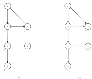
as the set of solutions which can be obtained from s by giving a color to a vertex x, while removing the color of all conflicting and r-conflicting vertices, with 2 ≤ r≤ i. Neighborhood N(3)(s) is illustrated in Figure 2.
a b c d e f a b c d e f 1 2 3 3 1 1 1 3 (i) (ii)
Fig. 2. (i) A partial legal solution s. (ii) A neighbor solution s0 in N(3)(s) obtained by assigning time period 1 to operation a.
5. Obtained results
In this section, we first propose a method which will be compared to our heuristics. Then we describe the way we generated instances. Finally, we present and discuss the obtained results.
5.1. Considered Methods for Numerical Comparisons
We propose now an integer linear program as well as a greedy algorithm.
The integer linear model associated with the M GCP is the following. Let G= (V, E, A) be a mixed graph
with V = {v1, . . . , vn}, E being the edge set and A
be-ing the arc set. Let C = {1, . . . , k} be the set of
avail-able colors. Let us define the following variavail-ables. For all i∈ {1, . . . , n} and j ∈ {1, . . . , k}, we set xij = 1
if vertex vigets color j and xij = 0 otherwise. For all
j ∈ {1, . . . , k}, we set zj = 1 if at least one vertex
gets color j and zj = 0 otherwise. The mixed graph
coloring problem can be defined as follows. The objec-tive function to minimize is
k
P
i=1
zi, and the constraints
Table 1
Graph |V | k∗ d dˆ Greedy Tabu VNS
DSJC250.1 250 8 0.1 0.001 9 (5) 8 (5) 8 (5) 0.002 9 (5) 8 (5) 8 (5) 0.003 9 (5) 8 (5) 8 (5) 0.005 9 (5) 8 (5) 8 (5) 0.01 9 (5) 8 (5) 8 (5) 0.05 13 (5) 13 (5) 13 (5) 0.1 30 (5) 30 (5) 30 (5) DSJC250.5 250 28 0.5 0.001 34 (5) 29 (5) 29 (5) 0.002 35 (5) 29 (4) 29 (3) 0.003 35 (5) 30 (5) 29 (2) 0.005 36 (5) 30 (1) 31 (4) 0.01 39 (5) 35 (5) 38 (1) DSJC250.9 250 72 0.9 0.001 84 (5) 72 (2) 72 (4) 0.002 84 (5) 73 (1) 73 (3) 0.003 87 (5) 74 (4) 74 (3) 0.005 89 (5) 78 (5) 82 (3) 0.01 95 (5) 91 (2) 97 (1) DSJR500.1 500 12 0.03 0.001 12 (5) 12 (5) 12 (5) 0.002 12 (5) 12 (5) 12 (5) 0.003 12 (5) 12 (5) 12 (5) 0.005 12 (5) 12 (5) 12 (5) 0.01 12 (5) 12 (5) 12 (5) 0.1 19 (5) 19 (5) 19 (5) DSJR500.1c 500 85 0.97 0.001 103 (5) 95 (1) 98 (2) 0.002 113 (5) 109 (2) 109 (1) 0.003 132 (5) 127 (2) 135 (1) 0.005 183 (5) 187 (1) 186 (1) 0.01 279 (5) 285 (3) 285 (4) DSJR500.5 500 122 0.47 0.001 127 (5) 126 (3) 127 (3) 0.002 130 (5) 127 (2) 129 (4) 0.003 132 (5) 127 (2) 129 (4) 0.005 137 (5) 132 (5) 138 (1) 0.01 146 (5) 149 (1) 148 (2) Results of the heuristics on the DSJC and DSJR graphs
xi1j+ xi2j ≤ 1∀[vi1; vi2] ∈ E, ∀j ∈ {1, . . . , k} (1) k X j=1 xij = 1∀vi∈ V (2) xij ≤ zj ∀vi∈ V, ∀j ∈ {1, . . . , k} (3) xi1j1+ xi2j2 ≤ 1 ∀(vi1; vi2) ∈ A, ∀j1≥ j2, j1, j2∈ {1, . . . , k} (4) xij, zj∈ {0, 1} ∀vi∈ V, ∀j ∈ {1, . . . , k} (5)
Constraints (1) impose that two vertices linked with an edge must get different colors; constraints (2) impose that each vertex must get exactly one color; constraints (3) are linking constraints; constraints (4) forbid to give a larger color to the start vertex of an arc than to the end vertex of an arc; constraints (5) impose integer values for variables xij and zj.
However, even if we use the CPLEX 10.2 MIP Solver (during one hour on the computer mentioned in section 5.), it can only manage very small and instances (up to 50 vertices), which are very easy to tackle with a local
search heuristic. This confirms that the use of heuris-tics is mandatory and thus no further comparison will be made with exact methods. Note that the same holds for the graph coloring problem: the best exact methods are able to tackle instances with up to 100 vertices, for which a tabu search procedure is able to find the optimal solution in a few seconds.
On the considered instances (with up to 500 vertices), we propose to compare Tabu-(P(k)) and VNS-(P(k))
with a simpler baseline heuristic, which will be a greedy heuristic, denoted Greedy-(P(k)), derived from Dsatur.
Dsatur [4] is a state-of-the-art greedy heuristic for the
GCP . First, the degree of a vertex x is the number of
adjacent vertices to x and the saturation degree of a vertex x is the number of different colors that are used by the vertices adjacent to x. Let Z be a set of ver-tices which is initialized to V . At each step and while
Z 6= ∅, Dsatur colors one vertex in Z as follows: (1)
select a vertex x∈ Z with the largest saturation degree
(break ties with the largest degree, and then randomly); (2) assign the smallest color to x without creating any conflict, and remove x from Z.
heuris-Table 2
Graph |V | χ(G) d dˆ Greedy Tabu VNS
le450 15c 450 15 0.16 0.001 23 (5) 16 (4) 16 (5) 0.002 23 (5) 17 (4) 17 (2) 0.003 23 (5) 17 (5) 18 (4) 0.005 24 (5) 18 (5) 18 (2) 0.01 25 (5) 21 (5) 22 (4) le450 15d 450 15 0.17 0.001 23 (5) 16 (4) 17 (5) 0.002 23 (5) 17 (5) 17 (5) 0.003 23 (5) 17 (1) 18 (5) 0.005 24 (5) 18 (5) 18 (2) 0.01 25 (5) 20 (1) 22 (1) le450 25c 450 25 0.17 0.001 28 (5) 27 (5) 27 (5) 0.002 28 (5) 27 (5) 27 (5) 0.003 28 (5) 27 (2) 27 (4) 0.005 29 (5) 28 (5) 27 (1) 0.01 30 (5) 29 (5) 29 (4) le450 25d 450 25 0.17 0.001 28 (5) 27 (5) 27 (5) 0.002 28 (5) 27 (4) 27 (5) 0.003 28 (5) 28 (5) 27 (2) 0.005 29 (5) 28 (5) 28 (5) 0.01 30 (5) 29 (5) 29 (4) flat300 20 0 300 20 0.47 0.001 38 (5) 21 (1) 22 (5) 0.002 38 (5) 23 (2) 23 (2) 0.003 39 (5) 25 (2) 26 (3) 0.005 40 (5) 27 (3) 27 (1) 0.01 42 (5) 32 (1) 40 (3) flat300 26 0 300 26 0.48 0.001 39 (5) 27 (5) 27 (3) 0.002 39 (5) 28 (3) 28 (1) 0.003 40 (5) 31 (5) 30 (5) 0.005 41 (5) 34 (4) 35 (1) 0.01 42 (5) 38 (5) 42 (2) flat300 28 0 300 28 0.48 0.001 39 (5) 32 (5) 30 (1) 0.002 39 (5) 33 (5) 33 (5) 0.003 39 (5) 33 (1) 33 (5) 0.005 40 (5) 35 (5) 35 (2) 0.01 44 (5) 40 (1) 45 (1) Results of the heuristics on the Leighton and flat graphs
Table 3
Tabu VNS Ties
All the 68 instances smaller k 21 7 40
larger success rate 11 7 22 13 instances with ˆd= 0.001 smaller k 4 1 8 larger success rate 1 2 5 13 instances with ˆd= 0.002 smaller k 1 0 12 larger success rate 4 2 6 13 instances with ˆd= 0.003 smaller k 5 3 5 larger success rate 1 2 2 13 instances with ˆd= 0.005 smaller k 4 2 7 larger success rate 4 0 3
13 instances with ˆd= 0.01 smaller k 7 1 5
larger success rate 1 1 3 33 instances with d close to 0.1 smaller k 5 2 26 larger success rate 4 3 19 20 instances with d close to 0.5 smaller k 8 3 9 larger success rate 5 1 3 10 instances with d close to 0.9 smaller k 4 1 5 larger success rate 2 3 0 Detailed comparison between Tabu-(P(k)) and VNS-(P(k))
tic for problem(P(k)), using only k colors. We change
the above step (2) as follows: we assign the smallest color of F C(x) to x without creating any conflict. If
no such color exists, we remove x from Z and we put
x in Ck+1, which is the set of non colored vertices.
The quality of a so obtained solution can be measured by |Ck+1|. If |Ck+1| = 0, the associated solution is
feasible. Otherwise, we only have a partial but legal solution. With such a method, the obtained results were not convincing at all. Thus, we propose the following improvement. In the above step (1), before considering the saturation degrees, we select vertex x∈ Z
accord-ing to the largest OutRank (ties are broken randomly). Thus, we start to color the vertices belonging to the longest paths of the considered graph.
In order to have a fair comparison, we use the same stopping condition for all the methods, which is a time limit of T= 60 minutes. As Greedy-(P(k)) needs much
less than 60 minutes to generate a solution, it will be restarted during 60 minutes, and the provided solution will be the best solution encountered during that time.
5.2. Generation of the Instances
In order to generate random mixed graphs from a non oriented graph G= (V, E), we process as follows. An
edge[x; y] is transformed into an arc with a probability
equal to ˆd, and if it is the case, it will be transformed
into an arc(x; y) or an arc (y; x) with an equal
prob-ability. Note that since we do not allow circuits in a mixed graph (otherwise there is no feasible solution), we only perform a transformation of an edge into an arc if the resulting arc does not create any circuit. If it does create a circuit, we then check the reverse orienta-tion. If both orientations create circuits, the considered edge will not be transformed into an arc.
We consider a set of 13 non oriented graphs from the most challenging ones (see [10]) of the DIMACS Chal-lenge (see ftp://dimacs.rutgers.edu/pub/chalChal-lenge/graph/). The orientation density ˆd is defined as the proportion of
oriented edges. Each of the 13 below mentioned graph is considered with ˆd∈ {0.001, 0.002, 0.003, 0.005, 0.01},
which results in 65 instances. In addition, for graphs DSJC250.1 and DSJR500.1, other values in{0.05, 0.1}
were also considered to better measure the augmen-tation of the number of required colors to color the graph. We consider four types of graphs:
• The DSJCn.10 · d instances are random graphs with
n vertices a density d, which means that each pair of
vertices has a probability of d to form an edge. We choose n= 250 and d ∈ {0.1, 0.5, 0.9}.
• The DSJRn.z instances are geometric random graphs
with n vertices, which are constructed by randomly choosing n points in the unit square and two vertices are connected if they are distant by less than z. Graphs with an added end letter ’c’ are the complementary graphs. We choose n= 500 and z ∈ {1, 5}.
• The flatn χ 0 instances are structured graphs with n
vertices and a chromatic number χ. The end number ’0’ means that all vertices are adjacent to the same
number of vertices. We choose n = 300 and χ ∈ {20, 26, 28}.
• The len χx instances are graphs with n vertices and
a chromatic number χ equal to the size of a largest clique (i.e., the largest number of pairwise adjacent vertices). The end letter ’x’ stands for different graphs with similar settings. We choose n = 450 and χ ∈ {15, 25}.
As such graphs have very different structures, sizes and densities, we believe that if the proposed heuristics per-form well on such instances, it will also be the case for other types of instances.
5.3. Presentation of the Results
Our algorithms were implemented in C++ and run on a computer with the following properties: Processor Intel Core2 Duo Processor E6700 (2.66GHz, 4MB Cache, 1066MHz FSB), RAM 2GB DDR2 667 ECC Dual Channel Memory (2x1GB).
The results are presented in Tables 2 for the random DSJC and DSJR graphs, and in Table 3 for the struc-tured Leighton and flat graphs. The five first columns respectively indicate the following information: the name of the graph, the number |V | of vertices, the
smallest number of colors k∗ for which a legal k∗ -coloring was found by a heuristic or the chromatic number χ(G) if it is known, the density d, and the
ori-entation density ˆd. The last three columns respectively
indicate the smallest number of colors for which a legal coloring was found by Greedy-(P(k)), Tabu-(P(k)),
and VNS-(P(k)), with the number of successes among
five runs (i.e. using five different seeds) in brackets. As expected, larger d and ˆd values lead to a larger number
of used colors.
VNS-(P(k)) are better than Greedy-(P(k)), which is not
surprising: a local search is in general better than a con-structive heuristic with restarts. On the other hand,
Tabu-(P(k)) outperforms VNS-(P(k)), which is not
straight-forward to understand: it actually means that the ingre-dients added to Tabu-(P(k)) to derive VNS-(P(k))
de-teriorates its behavior. More precisely, when performing and evaluating a move, i.e. when trying to color a ver-tex x, it is better to only focus on the vertices adjacent to x rather than to also consider more distant vertices. Therefore, the latter strategy does not help to guide the search and also needs extra computation.
It can be interesting to perform a more accurate com-parison between Tabu-(P(k)) and VNS-(P(k)),
accord-ing to several criterion: the nature of the graph (ran-dom or structured), the density d and the orientation density ˆd. This can be done based on the
informa-tion provided in Table 4, which was built from Ta-bles 2 and 3. The overall performance is first given: among the 68 considered instances, Tabu-(P(k)) found a
smaller legal k-coloring 21 times, VNS-(P(k)) 7 times,
and both methods obtained the same value of k 40 times. For these latter 40 instances, Tabu-(P(k)) had a
better success rate (among five runs) 11 times,
VNS-(P(k)) 7 times, and both methods obtained the same
success rate value 22 times. The same kind of infor-mation is then given for the instances with a fixed ˆd
value (with ˆd ∈ {0.001, 0.002, 0.005, 0.01}), then for
the instances with d close to 0.1 (i.e. the four Leighton graphs, DSJC250.1, and DSJR500.1), the instances with
d close to 0.5 (i.e. the three flat instances, DSJC250.5,
and DSJR500.5), and finally the instances with d close to 0.9 (i.e. instances DSJC250.9 and DSJR500.1c). We can generally see that the larger d or ˆd are (i.e. the more
complex the instance is), the better is Tabu-(P(k)) when
compared to VNS-(P(k)).
6. Conclusion
In this paper, we tackle a project scheduling problem
(P ) for which incompatibilities between operations
and precedence constraints are considered. The goal is to assign a time period to each operation while mini-mizing the duration, i.e. the number of time periods, of the project.
We showed that problem (P ) can be represented by
the mixed graph coloring problem, which is NP-hard. We propose three heuristics to tackle problem(P ): a
greedy procedure, a tabu search as well as a variable
neighborhood search.
Among the future work that can be done in that field, we mention two main avenues of research. In the first one, more sophisticated heuristics might be developed to tackle problem(P ). For example, one can derive
ef-ficient population based coloring heuristics in order to obtain better heuristics for(P ). In the second research
direction, one might design extensions of problem(P ),
such as the consideration of a specific duration for each operation, as well as various types of costs.
Acknowledgement: The present paper was partially
written while the second author was an assistant profes-sor at the Centre for Discrete Mathematics and its Ap-plications (DIMAP) at the University of Warwick. The support of the institution is gratefully acknowledged.
References
[1] F. S. Al-Anzi, Y. N. Sotskov, A. Allahverdi, and G. V. Andreev. Using Mixed Graph Coloring to Minimize Total Completion Time in Job Shop Scheduling. Applied Mathematics and Computation, 182(2):1137– 1148, 2006.
[2] C. Avanthay, A. Hertz, and N. Zufferey. A Variable Neighborhood Search for Graph Coloring. European Journal of Operational Research, 151:379–388, 2003. [3] I. Bloechliger and N. Zufferey. A Graph Coloring
Heuristic Using Partial Solutions and a Reactive Tabu Scheme. Computers & Operations Research, 35:960– 975, 2008.
[4] D. Br´elaz. New Methods to Color Vertices of a Graph. Communications of the Association for Computing Machinery, 22:251–256, 1979.
[5] E.L. Demeulemeester and W.S. Herroelen. Project Scheduling: A Research Handbook. Kluwer Academic Publishers, 2002.
[6] H. Furmanczyk, A. Kosowski, and P. Zylinski. A Note on Mixed Tree Coloring. to appear in Information Processing Letters, 2008.
[7] H. Furmanczyk, A. Kosowski, and P. Zylinski. Scheduling with Precedence Constraints: Mixed Graph Coloring in Series-Parallel Graphs. Lecture Notes in Computer Science, 4967:1001–1008, 2008.
[8] P. Galinier and J.K. Hao. Hybrid Evolutionary Algorithms for Graph Coloring. Journal of Combinatorial Optimization, 3 (4):379–397, 1999. [9] P. Galinier and A. Hertz. A Survey of Local Search
Methods for Graph Coloring. Computers & Operations Research, 33:2547–2562, 2006.
[10] P. Galinier, A. Hertz, and N. Zufferey. An Adaptive Memory Algorithm for the Graph Coloring Problem. Discrete Applied Mathematics, 156:267–279, 2008. [11] M. Garey and D.S. Johnson. Computer and
Intractability: a Guide to the Theory of NP-Completeness. Freeman, San Francisco, 1979.
[12] F. Glover and M. Laguna. Tabu Search. Kluwer Academic Publishers, Boston, 1997.
[13] P. Hansen, J. Kuplinsky, and D. de Werra. Mixed Graph Coloring. Mathematical Methods of Operations Research, 45:145–169, 1997.
[14] F. Herrmann and A. Hertz. Finding the chromatic number by means of critical graphs. ACM Journal of Experimental Algorithmics, 7 (10):1–9, 2002.
[15] A. Hertz and D. de Werra. Using Tabu Search Techniques for Graph Coloring. Computing, 39:345– 351, 1987.
[16] A. Hertz, M. Plumettaz, and N. Zufferey. Variable space search for graph coloring. Discrete Applied Mathematics, 156:2551 – 2560, 2008.
[17] H. Kerzner. Project Management: A Systems Approach to Planning, Scheduling, and Controlling. Wiley, 2003. [18] E. Malaguti, M. Monaci, and P. Toth. A Metaheuristic Approach for the Vertex Coloring Problem. INFORMS Journal on Computing, 20 (2):302 – 316, 2008. [19] N. Mladenovic and P. Hansen. Variable neighborhood
search. Computers & Operations Research, 24:1097– 1100, 1997.
Received 14-4-2010; revised 4-8-2010; accepted 19-8-2010
[20] C. Morgenstern. Distributed Coloration Neighborhood Search. DIMACS Series in Discrete Mathematics and Theoretical Computer Science, 26:335–357, 1996. [21] M. Pinedo. Scheduling: Theory, Algorithms, and
Systems. Prentice Hall, 2002.
[22] M. Plumettaz, D. Schindl, and N. Zufferey. Ant local search and its efficient adaptation to graph colouring. Journal of the Operational Research Society, 61:819 – 826, 2010.
[23] B. Ries. Coloring some classes of mixed graphs. Discrete Applied Mathematics, 155:1–6, 2007.
[24] B. Ries. Variations of coloring problems related to scheduling and discrete tomography. PhD thesis,
´
Ecole Polytechnique F´ed´erale de Lausanne (EPFL), Switzerland, 2007.
[25] B. Ries. Complexity of Mixed Graph Coloring. Discrete Applied Mathematics, 158: 592-596 (2010).
[26] B. Ries and D. de Werra. On Two Coloring Problems in Mixed Graphs. European Journal of Combinatorics, 29(3):712–725, 2008.
[27] Y. N. Sotskov. Scheduling via Mixed Graph Coloring. In Operations Research Proceedings, September 1–3, 1999, Springer Verlag, pages 414–418, 2000.
[28] Y. N. Sotskov, A. Dolgui, and F. Werner. Mixed Graph Coloring for Unit-Time Job-Shop Scheduling. International Journal of Mathematical Algorithms, 2:289–323, 2001.