Leveraging the network: A stress-test framework based on DebtRank

Research Article

Stefano Battiston*, Guido Caldarelli, Marco D’Errico and Stefano Gurciullo

Leveraging the network:

A stress-test framework based on DebtRank

Received February 27, 2015; revised February 22, 2016; accepted July 26, 2016

Abstract: We develop a novel stress-test framework to monitor systemic risk in financial systems. The modu-lar structure of the framework allows to accommodate for a variety of shock scenarios, methods to estimate interbank exposures and mechanisms of distress propagation. The main features are as follows. First, the framework allows to estimate and disentangle not only first-round effects (i.e. shock on external assets) and second-round effects (i.e. distress induced in the interbank network), but also third-round effects induced by possible fire sales. Second, it allows to monitor at the same time the impact of shocks on individual or groups of financial institutions as well as their vulnerability to shocks on counterparties or certain asset classes. Third, it includes estimates for loss distributions, thus combining network effects with familiar risk measures such as VaR and CVaR. Fourth, in order to perform robustness analyses and cope with incomplete data, the framework features a module for the generation of sets of networks of interbank exposures that are coherent with the total lending and borrowing of each bank. As an illustration, we carry out a stress-test exercise on a dataset of listed European banks over the years 2008–2013. We find that second-round and third-round effects dominate first-round effects, therefore suggesting that most current stress-test frameworks might lead to a severe underestimation of systemic risk.

Keywords: Systemic risk, leverage network, stress-test MSC 2010: 91B30

1 Introduction

The financial crisis has boosted the development of several network-based methodologies to monitor systemic risk in the financial system [10, 27, 28, 35, 44, 45, 49, 51, 53].

A traditional approach towards the quantification of systemic risk is to measure the effects of a shock on the external assets of each institution and then to aggregate the losses. However, the crisis has highlighted that stress-testing should also incorporate so-called “second-round” effect, which might arise via interbank exposures, either as losses on the asset side or liquidity shortages (see e.g. [7] and references therein). For instance, the recent ECB comprehensive assessment carried out in 2014 [29] goes into this direction by taking into account counterparty credit risk while the Basel III framework [5] gives attention to interconnectedness as a key source of systemic risk.

Some network-based methods focus on the events of a bank’s default (i.e. its equity going to zero) as the only relevant trigger for the contagion to be passed on to the counterparties. In other words, an institution

*Corresponding author: Stefano Battiston: Department of Banking and Finance, University of Zurich, Plattenstrasse 14,

8032 Zürich, Switzerland, e-mail: stefano.battiston@bf.uzh.ch

Guido Caldarelli: IMT Alti Studi Lucca, ISC-CNR, Rome, Italy; and LIMS London, Great Britain,

e-mail: guido.caldarelli@imtlucca.it

Marco D’Errico: Department of Banking and Finance, University of Zurich, Plattenstrasse 14, 8032 Zürich, Switzerland,

e-mail: marco.derrico@uzh.ch

that has faced some shocks will not affect its counterparties in any way as long as it is left with some positive equity. This is a useful simplification which has allowed for a number of mathematical developments [38]. Because regulators recommend banks to keep their largest single exposure well below their level of equity, most stress tests conducted in this way yield essentially to the result that a single initial bank default never triggers any other default. Systemic risk emerges only if, at the same time, one assumes a scenario of weak balance sheets [45] or a scenario of fire sales [58].

In contrast, both the intuition and the classic Merton approach, suggest that the loss of equity of an insti-tution, even with no default, will imply a decrease in the market value of its obligations to other institutions. In turn, this means a loss of equity for those institutions, as long as they revalue their equity as the difference between assets and liabilities. Therefore, financial distress, meant as loss of equity, can spread from a bank to another although no default occurs in between. The total loss of equity in the system can be substantial even if no bank ever defaults in the process. Indeed, in the 2007/2008 crisis, losses due to the mark-to-market re-evaluation of counterparty risk were much higher than losses due from direct defaults.¹ The so-called DebtRank methodology has been developed with the very idea to capture such a distress propagation [10]. The impact of a shock, as measured by DebtRank, is fully comparable to the traditional default-only propaga-tion mechanisms [27, 57] in the sense that the latter is a lower bound for the former. In other words, DebtRank measures at least the impact that one would have with the defaults-only, but it is typically larger and this al-lows to assign a level of systemic importance in most situations in which the traditional method would be unable to do so because the impact would be zero for all banks. DebtRank has been applied to several empir-ical contexts [3, 10, 26, 30, 55, 56, 63] but it was not so far been embedded into a stress-test framework. In this paper, building on the method introduced in [10], we develop a stress-test framework aimed at providing central bankers and practitioners with a monitoring tool of the network effects. The main contributions of our works are as follows.

First, the framework delivers not only an estimation of first-round (shock on external assets), and second-round (distress induced in the interbank network) effects, but also a third-second-round effect consisting in possible further losses induced by fire sales. To this end we incorporate a simple mechanism by which banks deter-mine the necessary sales of the asset that was shocked in order to recover their previous leverage level and assuming a linear market impact of the sale on the price of the asset. The three effects are disentangled and can be tracked separately to assess their relative magnitude according to a variety of scenarios on the initial shock on external assets and on liquidity of the asset market. Second, the framework allows to monitor at the same time the impact and the vulnerability of financial institutions. In other words, institutions whose default would cause a large loss to the system become problematic only if they are exposed to large losses when their counterparties or their assets get shocked. These quantities are computed through two networks of leverage that are the main linkage between the notion of capital requirements and the notion of interconnectedness. Third, the framework allows to estimate loss distributions both at the individual bank level and at the global level, allowing for the computation of individual and global VaR and CVaR (Table 2). Fourth, since data on bilateral exposures are seldom available, the framework includes a module to estimate the interbank network of bilateral exposures given the information on the total lending and borrowing of each bank. Here, we use a combination of fitness model [18, 19, 25, 51, 52] for the network structure and an iterative fitting method to estimate the lending volumes, but alternative methods could be used or added as benchmark comparison (e.g. the maximum entropy method [50, 65] or the minimum density method [2]). Finally, the framework has been developed in MATLAB and is available upon request to the authors. As an illustration, we carry out a stress-test exercise on a dataset of 183 European banks over the years 2008–2013, starting from the estimation of their interbank exposures.

This paper is organized as follows. In Section 1.1 we review similar or related work. In Section 2 we describe the main aspects of the framework, providing an outline of the distress process, a discussion of

1 See, as a reference, the Basel Committee on Banking Supervision, observing that “roughly two-thirds of losses attributed to counterparty credit risk were due to CVA losses and only about one-third were due to actual defaults.” www.bis.org/press/ p110601.htm

the main variables, and the framework’s building blocks. In Section 3, we show how the framework can be applied to a dataset and we discuss the main results of this exercise. In Section 4, we review the main contributions and introduce elements for future research. In Appendix A, we provide the technical details of the distress propagation process, including how the key measures are computed. In Appendix B, we describe the data we used for the exercise in Section 3. Finally, in Appendix C, we outline the network reconstruction methods when only the total interbank lending/borrowing for each bank is known.

1.1 Related work

The recent – and still ongoing – economic and financial crisis has made clear the importance of methods of early detection of systemic risk in the financial system. In particular, researchers, regulators and policy-makers have recognized the importance of adopting a macroprudential approach to understand and mitigate financial stability. Notwithstanding the many efforts [41], regulators still lack an adequate framework to mea-sure and address systemic risk².

The traditional micro-prudential approach consists in trying and ensuring the stability of the banks, one by one, with the assumption that as long as each unit is safe the system is safe. This approach has demon-strated to be a dangerous over-simplification of the situation [13]. Indeed, we have learned that it is precisely the interdependence among institutions, both in terms of liabilities or complex financial instruments and in terms of common exposure to asset classes what leads to the emergence of systemic risk and makes the prediction of the behavior of financial systems so difficult [9]. While risk diversification at a single institution can indeed lower its individual risk, if all institutions behave in a similar way, herding behavior can instead amplify the risk. Clearly, if all banks take similar positions, the failure of one bank can cause a global distress [14, 15, 62], because of the increased sensitivity to price changes [54]. To add more complexity, the causes of market movements are still under debate [21, 23], suggesting that exogenous instabilities add up to en-dogenous ones [24]. The tension between individual regulation and global regulation [11] poses a series of challenging questions to researchers, practitioners and regulators [4].

Traditionally, well before the recent crisis, it was argued that systemic risk is real when contagion phe-nomena across countries take place [12, 42]. In this spirit, a series of studies dealt with the description of systemic risk in the financial system from the perspective of the contagion channels across balance-sheet of several institutions [28, 32, 34, 37, 49, 51]. In particular, some focus was drawn upon the topology of connections (or the network [16]) between institutions [1, 27, 58].

In this way, the problem of analyzing systemic risk splits in two distinct problems [20]. First, the problem of understanding the role of an opaque (if not unknown) structure of financial contracts [17] and, second, the problem of providing a measure for the assessment of the impact of a given shock [10]. As for the first prob-lem, the obvious starting point is to consider the structure of the interbank network [25, 40, 46, 50, 59], with the aim of possibly extracting some early warning signals [61]. While many argued that the network struc-ture can be intrinsically a source of instability, it turns out instead that no specific topology can be considered as systematically safer than the others [58]. Indeed, only the interplay between market liquidity, capital re-quirements and network structure can help in the understanding of the systemic risk [43, 58]. For the second problem, researchers have tried to describe the dynamics of propagation of defaults with various methods, including by means of agent-based models [33] or by modelling the evolution of financial distress across balance-sheets conditional upon shocks in one or more institutions [10].

From the perspective of financial regulations, capital requirements represent the cornerstone of pruden-tial regulations. Institutions are required to hold capital as a buffer to shocks of any nature. The most used risk measures (such as Value at Risk and Expected Shortfall) are indeed related to the quantity of cash each individual bank needs to set aside in order to cover the direct exposures to different types of risk. In such manner, the indirect exposures arising from the interconnected nature of the financial system are not

consid-2In the following, we refer to systemic risk to indicate the probability that a large portion of the financial system is in distress or collapses.

ered. Interconnectedness, though, is now entering the debate on regulation: for example, the definition of “Global Systemically Important Banks” (G-SIBs [6]) does include the concept of interconnectedness, thereby measured as the aggregate value of assets and liabilities each bank has with respect to other banking institu-tions. Although this represents a fundamental step towards the inclusion of interconnectedness in assessing systemic risk, a further level of disaggregation would be needed. In fact, institutions that are similar in terms of their aggregated exposures (including those vis-à-vis other financial institutions), might have completely different sets of counterparties, therefore implying different levels of systemic impact and/or vulnerability to shocks. Another important point is that the potential negative effects arising from interconnectedness ought to be included into the definition of capital requirements.

2 The DebtRank stress-test framework

In this section, we introduce and describe the DebtRank stress-test framework. One of the main characteristics of the framework lies in its flexibility along the following four main dimensions:

∙ Shock type. The framework can implement different shock types and scenarios (on external assets). ∙ Network estimation. When detailed bilateral interbank exposures are not available, the framework

pro-vides a module to estimate the interbank network from the total interbank assets and liabilities of each bank.

∙ Contagion dynamics. The framework can implement two different contagion dynamics, distress contagion and default contagion.

∙ Systemic risk indicators. The framework returns as output a series of systemic risk indicators, both at the individual and a the global level. The user can aptly combine this information to extract the informa-tion needed. Several graphical outputs are also available and represent a key feature of the framework: graphics are specifically designed to capture relevant information at a glance.

Given the flexibility of the framework and the number of outputs produced, in the remainder of the sec-tion, we focus on:

∙ describing the main features of the DebtRank distress process as the key foundation of the framework; ∙ providing a qualitative description of the main variables of interests;

∙ providing a technical summary of the building blocks of the framework, which include the inputs required, the outputs that can be obtained and the different modules constituting the framework.

The reader can find detailed information about the process and the main variables of interest in the methodological Appendix A.

2.1 Outline of the distress process

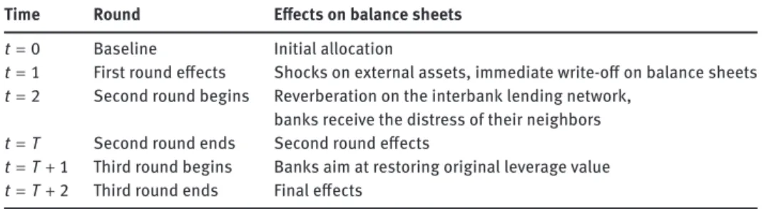
One of the key concerns in the measurement of systemic risk is to quantify losses at the individual and global level. In particular, DebtRank focuses on the depletion of equity when banks experience losses in external or interbank assets. We envision a system of n banks (indexed by i = 1, . . . , n) and m external assets (indexed by k = 1, . . . , m). The framework features a dynamic distress model, with t = 0, 1, . . . , T, T + 1, T + 2: ∙ Initial configuration. At time t = 0, banks allocate their uses and sources of funding, all variables at this

time represent the initial conditions of the process.

∙ First round. At time t = 1, we assume a negative shock on the value of one or more assets k. Banks imme-diately record the loss and, as they have to pay back their liabilities, reduce their equity level accordingly. We refer to these losses in equity as first-round effects.

∙ Second round. Given the equity loss of each bank, the likelihood of a bank repaying its obligations on the interbank lending market becomes lower, therefore reducing the market value of its obligations. This triggers effects on the interbank lending network. Indeed, from t = 2 to t = T ≥ 2, we model the prop-agation of distress in the interbank network. We refer to the loss on equity at this point as second-round effects. At at certain time t = T, the second round ends.

Time Round Effects on balance sheets

t = 0 Baseline Initial allocation

t = 1 First round effects Shocks on external assets, immediate write-off on balance sheets

t = 2 Second round begins Reverberation on the interbank lending network, banks receive the distress of their neighbors

t = T Second round ends Second round effects

t = T + 1 Third round begins Banks aim at restoring original leverage value

t = T + 2 Third round ends Final effects

Table 1. The distress dynamics.

∙ Third round. From time t = T + 1, the equity level is reduced from the initial configuration and banks aim at restoring the original leverage levels. In order to do so, they sell external assets (fire sales). This triggers further effects on the price of external assets and reduces equity levels to a greater extent. We refer to these losses as third-round effects.

Our framework is based on the clear separation between rounds of distress. At each round, the loss in equity is the key variable in our framework. As a quick reference, a summary of the distress dynamics is provided in Table 1.

2.2 Measuring systemic risk: The main variables

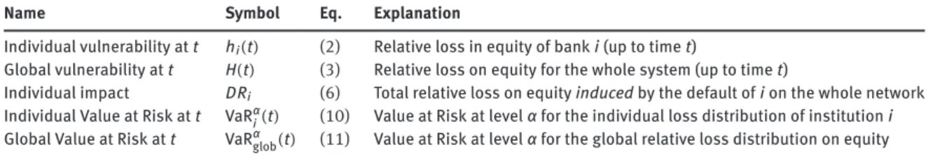
We now give a brief description of the main variables in the framework, and their interpretation in terms of systemic risk. As a reference, the reader can find a summary of these variables in Table 2.

Vulnerability. As previously noted, the key quantity in the framework is the loss in equity for each bank at each time t. In terms of systemic risk, however, there is substantial difference between the loss in equity a bank suffers and the loss in equity a bank induces in the system. We call the first variable the vulnerability of a bank and the second variable the impact of a bank onto the system as a whole. More formally, given the equity values at the initial configuration Ei(0), we define the individual vulnerability hi(t) of bank i at t as follows:

hi(t) = min{1,

Ei(0) − Ei(t) Ei(0) }.

The bank defaults when hi(t) = 1. Similarly, we can compute the global vulnerability of the system at time t, by taking the weighted average of hi(t), with weights given by the relative initial equity:

H(t) = n ∑ i=1 ( Ei(0) ∑jEj(0) hi(t)).

Impact. Institutions in a financial system are not only systemically relevant in terms of the shock they receive but also in terms of the loss they cause in case of their default. We call the individual impact of an institution i, the relative equity loss induced by the default of i (as computed in (6) in the methodological Appendix A). We denote the impact with DRias it is consistent with the original DebtRank approach introduced in [10]. Notice that the measure of impact naturally applies only to the distress a bank induces in the interbank network. Loss distributions. Conditioning to specific shocks, one can characterize a loss distribution both at the in-dividual level hi(t) and at the global level H(t) at each time t. In this context, “loss” and “vulnerability” can be used interchangeably. Notice that both the notions of individual and global loss distribution are key as-pects in the quantification of systemic risk. As a matter of fact, a large fraction of the global losses may be attributable to a few key banking institutions. In particular, we compute the Value at Risk (VaR) and the Con-ditional Value at Risk (CVaR), as these measures have emerged as some of the key tools for risk assessment. In our framework, these measures move towards the inclusion of network effects. In addition, the global loss distribution provides a clear understanding of the vulnerability of the system as a whole conditional to a specific shock.

Name Symbol Eq. Explanation

Individual vulnerability at t hi(t) (2) Relative loss in equity of bank i (up to time t)

Global vulnerability at t _H(t) (3) Relative loss on equity for the whole system (up to time t)

Individual impact DRi (6) Total relative loss on equity induced by the default of i on the whole network

Individual Value at Risk at t VaRα_i(t) (10) Value at Risk at level α for the individual loss distribution of institution i Global Value at Risk at t VaRα_glob(t) (11) Value at Risk at level α for the global relative loss distribution on equity

Table 2. Description of the main variables in the stress-test framework.

Input Banks’ balance sheets → (i) lending/borrowing (interbank vs total) (ii) external assets (with possible breakdowns) (iii) equity (and reserve capital in general) Shock scenario → (i) one or more banks

(ii) one or more asset classes

Output Results of modelling scenario → Contagion (DebtRank, default cascade)

Exposure estimation (fitness model, null models, maximum entropy, minimum density)

Table 3. Building blocks of the stress-test framework.

Evolution in time. All measures of vulnerability/losses and impact both at the individual and global level can be tracked over time, therefore providing a way to monitor the evolution of key figures in terms of systemic risk. In the exercise reported in Section 3, we focus on the monitoring of these key variables for a subset of 183 European banks in the years from 2008 to 2013. The dynamics of these key systemic risk variables allows to capture the evolution of systemic risk in time.

2.3 The framework’s building blocks

Since the DebtRank stress-test framework features several quantitative and graphical outputs for input data that are usually publicly available, we now provide a brief, yet comprehensive, overview of the main building blocks. We use Table 3 as the main reference.

2.3.1 Input

Input – data on balance sheets. The fundamental input data are represented by banks’ balance sheets. In particular, the framework takes the equity, the total asset value and the total interbank lending and borrowing of each bank as minimal inputs. More granular data on the structure of external assets are indeed possible (e.g. in case one wants to simulate a shock on a specific asset class).

Input – shock scenario. The flexibility of the modeling framework allows for a number of shock scenarios, including:

∙ a fixed shock (e.g. 1%) on the value of all external assets;

∙ a shock on the value of all external assets drawn from a specific probability distribution (e.g. a Beta distribution, which we use in the exercise in Section 3);

∙ when more detailed information on the holdings in external assets for banks is available, the shock (either fixed or drawn from a probability distribution) on specific asset classes.³

3 This also allows to run the stress test by applying heterogenous shocks with a pre-determined correlation structure. However, we will tackle this issue more specifically in future works.

2.3.2 Output

Output – results. As outlined above, the framework allows to compute the main systemic risk variable for two main types of contagion dynamics:

∙ The default cascade dynamics: banks impact other banks only in case of their default (see, for the tech-nical details, the discussion related to (4) in the methodological Appendix A).

∙ The DebtRank dynamics: banks impact other banks regardless of whether the event of default occurred. The rationale behind this type of dynamics is that, as banks reduce their equity levels to face losses, they decrease their distance to default and therefore are less likely to repay their obligations. In this case, the market value of their obligations is reduced and is hence reflected on the asset side of their counterparties in the interbank market.

Output – bilateral exposures estimation. As detailed data on banks’ bilateral exposures are often not pub-licly available, estimations need to be performed in order to run the framework. Even though such estimations constitute a key input of the stress test framework in case the exposures are not known, they constitute an output on their own, because they can be then analyzed with the typical tools of network analysis. Also, the estimations can serve for two other purposes: (i) as a benchmark for comparison with the observed data, à la Savage and Deutsch [60], or (ii) for the estimation of missing data [2]. From a technical viewpoint, the methodology we use to estimate the interbank network is based on the so-called “fitness model” [25, 52]. The technical details are reported in Appendix C.

3 The framework at work: Results of a stress test exercise

In order to show how the framework works and what type of outputs are available, in this section we apply the framework to a specific dataset of 183 EU banks for the years 2008–2013. More details on the dataset are available in Appendix B. In brief:

∙ We collect yearly data on equity, external assets, interbank assets and liabilities for the set of banks under scrutiny.

∙ We estimate the exposures by combining the fitness model and an iterative fitting procedure (Ap-pendix C), generating (for each year) 100 networks compatible with the total interbank borrowing and lending of each bank at end-year.

∙ We then run the stress test in order to obtain the main systemic risk variables for all years. When not explicitly specified, the statistics reported in this section are computed by taking the median value of the 100 networks.

In the remainder of this section, we describe the main results, including some key charts and figures, in order to show part of the graphical output of the framework.

3.1 Vulnerability and impact

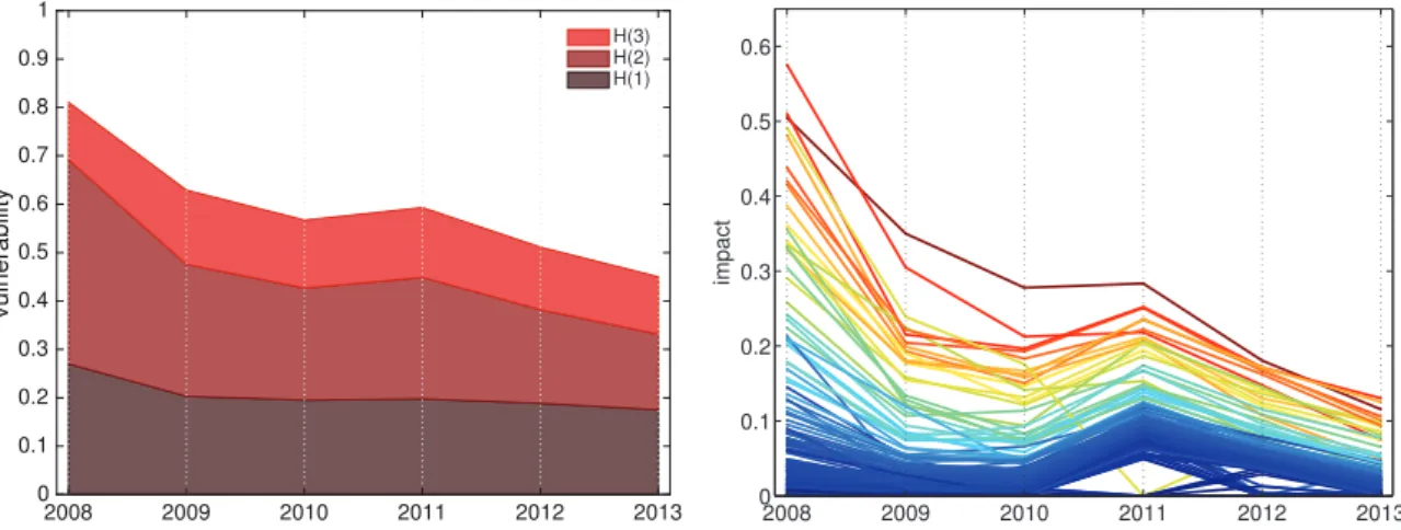
Figure 1 provides an overview of the response of the reconstructed financial networks and its individual ele-ments to the distress scenarios simulated. The chart on the left shows the dynamics of global equity losses (H) from 2008 to 2013, the values reported are the median value of H across the 100 networks in the Monte Carlo sample and are computed for a common shock of 1% on the external assets. The chart also offers a deconstruc-tion of the losses, according to if they are caused by the first (external assets shocks), second (reverberadeconstruc-tion on the interbank lending network), and third (fire sales) round of distress propagation. The relative losses in equity due to the second and third rounds are substantial, implying that an assessment of systemic risk solely based on first-round effects is bound to underestimate potential losses. The chart on the right shows the evo-lution of the impact for each of the 183 banks in the sample throughout the years. Each line is the median of the impact calculated over the 100 networks in the ensemble. The plot clearly shows a general decrease in

2008 2009 2010 2011 2012 2013 0 0.1 0.2 0.3 0.4 0.5 0.6 0.7 0.8 0.9 1 vulnerability H(3) H(2) H(1) impact 2008 2009 2010 2011 2012 2013 0 0.1 0.2 0.3 0.4 0.5 0.6

Figure 1. Systemic vulnerability and individual impact over time. Left: Plot of the global vulnerability in time and its

decompo-sition with respect to the different rounds. Right: Individual impact over time. In order to show that impactful institutions keep being so during the years, colors reflect the impact in 2008.

the systemic impact for the individual institutions over time. In order to visually capture the persistency over time of banks with higher or lower impact, the colors reflect the level of the average impact computed over the years. In particular, red lines are associated to banks that consistently show a high impact. Conversely, blue lines are associated to banks that have a consistently low impact. We observe a certain level of stability of the relative levels: banks which show a higher systemic impact tend to do so throughout the years.

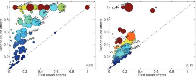
From a systemic risk perspective, it is of particular interest to compare the two main systemic risk quanti-ties associated to each individual bank: the vulnerability to external shocks and the impact of a bank onto the system in case of its default. By jointly analyzing these two quantities, we divide institutions into four main categories: (i) high vulnerability/high impact, (ii) high vulnerability/low impact, (iii) low vulnerability/low impact, (iv) low vulnerability/high impact.

Results for this exercise are reported in Figure 2. The graphs report a plot of the vulnerability hiat the second round versus the impact DRifor each year in the sample. The [0, 1] × [0, 1] square is divided into four quadrants, which correspond to the aforementioned four categories. Interbank leverage and total asset size are respectively visualized by node color (red implies high leverage, blue otherwise) and node size. Both interbank leverage and asset size appear to be associated with high values of vulnerability and impact. We observe an interesting phenomenon: in 2008, a high number of large (in terms of asset size) institutions are both highly vulnerable (up to their default) and impactful (up to 70% of the total initial equity). Their systemic relevance is therefore extremely high, as they have higher likelihood to receive distress. In turn, once the distress has been received, they would have a great impact on the rest of the system. The situation improves over time and, in 2013, no bank is in the upper right quadrant. Some financial institutions retain, though, very high vulnerability and significant impact. A financial institution that can cause a global relative equity loss of 10% still acts as a source of systemic risk not to be ignored. However, some large institutions are still prone to receive high level of distress, and nevertheless keep a significant impact (up to 20% on the rest of the system). We also notice that those institutions which are both vulnerable and impactful are generally large and very large ones in terms of asset size.

3.2 Decomposition of first- and second-round effects

Figure 3 shows a way of visualizing the decomposition of first- and second-round effects. Again, we compare the years 2008 (left) and 2013 (right). The x-axis plots the losses at the first round and the y-axis the losses after the second round. Since the losses at the second round include the ones at the first, points must lie above the line bisecting the first quadrant. Nodes lying on the line itself are isolated in all the artificially generated networks. We observe a significant reduction in the effects. As usual, the color reflects the interbank leverage

0 0.2 0.4 0.6 0.8 1 0 0.1 0.2 0.3 0.4 0.5 HSBC BNP DB Barclays Cred. Agric. vulnerability impact 2008 0 0.2 0.4 0.6 0.8 1 0 0.1 0.2 0.3 0.4 0.5 HSBC BNP DB Barclays Cred. Agric. vulnerability impact 2013

Figure 2. Individual vulnerability vs individual impact (2008 and 2013) Circle size reflects asset size, colors reflect the

magnitude of the interbank leverage. The four quadrants divide the banks into four categories.

0 0.2 0.4 0.6 0.8 1 0 0.2 0.4 0.6 0.8 1 RBS DB Barclays BNP HSBC Cred. Agric. ING Soc. Gen. Santander Unicred.

First round effects

Second round effects

2008 0 0.2 0.4 0.6 0.8 1 0 0.2 0.4 0.6 0.8 1 HSBCBNP DB Barclays Cred. Agric. Soc. Gen. RBS Santander ING _Lloyds

First round effects

Second round effects

2013

Figure 3. Decomposition of first- and second-round effects in 2008 and 2013 for an initial shock on external assets r(1) = 0.01.

The names of the first top ten institutions by asset size for each year are shown.

and circle diameter the asset size. Consistently with the findings in Appendix A, nodes with higher interbank leverage typically suffer more losses in the second round.

3.3 Distribution of losses

3.3.1 Global losses

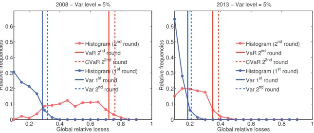
We evaluate a distribution of relative global equity losses by simulating 150 different systemic shock levels drawn from a Beta distribution.⁴ Figure 4 shows the distributions resulting by taking into account first-round only (blue lines) and second-round (red lines) distress propagation effects for the years 2008 and 2013. Ver-tical lines indicate VaR values at 95%, dashed lines are CVaR at the same level (see Appendix A.4 for details). An extremely important consideration can be made from this figure: accounting for second-round effects greatly increases the likelihood of having larger global equity losses, thus shifting VaR values towards the right. In 2008, a scenario where only first-round distress is induced leads to a relatively low VaR level. This,

4_{The parameters of the Beta distribution chosen are a = 4 and b = 8 respectively. The distribution has been then truncated in}

0.2 0.4 0.6 0.8 1 0 0.1 0.2 0.3 0.4 0.5 0.6

Global relative losses

Relative frequencies 2008 − Var level = 5% Histogram (2nd round) VaR 2nd round CVaR 22nd round Histogram (1st round) Var 1st round Var 2nd round 0.2 0.4 0.6 0.8 1 0 0.1 0.2 0.3 0.4 0.5 0.6

Global relative losses

Relative frequencies 2013 − Var level = 5% Histogram (2nd round) VaR 2nd round CVaR 22nd round Histogram (1st round) Var 1st round Var 2nd round

Figure 4. Distribution of global relative losses (global vulnerability) in 2008 and 2013. Relative shocks on value of external

assets drawn from a Beta distribution with parameters [4, 8] and truncated with a maximum of 0.015.

0.1 0.2 0.3 0.4 0.5 0.6 0.7 0.8 0.9 0 0.05 0.1 0.15 0.2 0.25 0.3 0.35 0.4 0.45 0.5 Loss distribution Relative frequencies

2013 − bank: IntesaSanPaolo, 5% VaR

Histogram (2nd round) VaR (2nd round) CVaR (2nd round) Histogram (1st round) VaR (1nd round) CVaR (2nd round) 0.1 0.2 0.3 0.4 0.5 0.6 0.7 0.8 0.9 0 0.05 0.1 0.15 0.2 0.25 0.3 0.35 0.4 0.45 0.5 Loss distribution Relative frequencies 2013 − bank: HSBC, 5% VaR Histogram (2nd round) VaR (2nd round) CVaR (2nd round) Histogram (1st round) VaR (1nd round) CVaR (2nd round)

Figure 5. Individual losses for two large banks. The chart reports the loss distribution for Intesa SanPaolo (left)

and HSBC (right).

instead, reaches a much higher value after the second-round effect is added. A similar, though less extreme, pattern is found in 2013. The observed VaR shift phenomenon is another compelling piece of evidence stating that systemic risk measures ought to take into account network effects.

3.3.2 Individual losses

Figure 5 shows yet one of the outputs of the framework: the distribution of losses can be obtained for each individual bank. Here, we focus on two large institutions (by asset size): HSBC (which ranks first by asset size in 2013) and Intesa SanPaolo (which ranks thirteenth in 2013). Despite the difference in asset size, the original distances in the levels of VaR for the first round (0.15 vs 0.14) become much more relevant when second-round effects are considered (0.28 vs 0.22). The example shows that significant differences in terms of standard risk measures are missed out if we neglect second-round effects.

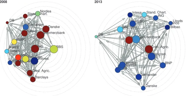
HSBC BNP DB Barclays Cred. Agric. Soc. Gen. RBS Santander ING Lloyds Unicred. Nordea Intesa Banco Bilbao Commerzbank Natixis Stand. Chart. Danske 2008 HSBC BNP DB Barclays Cred. Agric. Soc. Gen. RBS Santander ING Lloyds Unicred. Nordea Intesa Banco Bilbao Commerzbank Natixis Stand. Chart. Danske 2013

Figure 6. Network visualization of the top 18 institutions by asset size in 2008 and 2013. Nodes are positioned on the

concentric circles according to their Katz centrality.

4 Discussion and concluding remarks

The exercise carried out in Section 3 shows how the framework can be used to compute a variety of individual and global quantities that are relevant to systemic risk. The framework allows for a number of additional analyses which are not reported in detail in this paper for the sake of conciseness. For instance, Figure 6 represents one of the outputs of the framework in terms of network visualization and allows to compare the network position of individual institutions with other information. In this example, the interbank exposures among the top 18 banks by total asset size in 2008 (left) and 2013 (right) are considered. The position of a bank in the chart is determined by its impact: the higher the impact, the more central the bank is located in the circle. The bubble size is proportional to total asset size of the bank, while the color encodes its vulnerability (on a scale from blue to red, red nodes are more vulnerable). It is worth mentioning the discussion on the determinants of the systemic importance of financial institutions. In particular, one question is to what extent the asset size of an institution can be a good predictor of the impact of the bank on the system as a whole, and how much we should instead consider the position of the bank in the interbank network. Previous work have found that, although systemically important banks are typically among the large banks, banks with similar size can have very different impact on the system, in case of default [26]. In line with those results, in our exercise, we find, loosely speaking, that asset size is not a good predictor of impact (i.e. the Pearson correlation between asset size and individual impact, as measured by DebtRank, for the top 30 institutions by total assets, each year is quite low, around 0.5).

To summarize, this paper presents a stress-test framework focused on the evaluation of network effects in systemic risk. We have illustrated how to carry out a stress-test exercise on a dataset of 183 European banks over the years 2008–2013. The code underlying the framework has been developed in MATLAB and is available upon request to the authors.

The notion of interconnectedness has already entered the debate on “Global Systemically Important Banks” (G-SIBs [6]). However, this notion has been meant so far in an aggregate sense, without fully recog-nizing that institutions with similar aggregated exposures can have very different levels of systemic impact and/or vulnerability to shocks. Indeed, a central notion in our framework is the one of leverage networks, i.e. the set of leverage relations among banks’ balance-sheets and among banks and assets. The effect of these relations is the key starting point to monitor systemic risk from a network perspective. Accordingly, our

frame-work allows to track separately the magnitude of the so-called first-, second- and third-round effects, a feature that is particularly important in the discussion of future stress tests at national and international level. In this respect, in line with previous work on German interbank data [30], we find that the second-round effect is at least as large as the first-round effect.

Notice that by adopting traditional analyses based on default-only mechanisms [27, 57], we would in-stead find very limited second-round effects. There are two main reasons for this discrepancy. First, in a default-only framework the propagation of distress only occurs in the case of outright default. For example, in order to trigger any second-round effect, at least one default in the first round is necessary: this would in turn imply that an initial shock needs to be at least as large as the reciprocal of a bank’s leverage (see Appendix A). In order for the second round to be significant, there would need to be a large number of defaults in the first round. Indeed, banks are recommended to keep their single largest exposure well below their capital so that a necessary condition for second-round losses is the default of at least two of their counterparties. However, in the practice, banks regularly re-evaluate their mark-to-market exposures to their counterparties in order to take into account the changes in their probability of default (i.e. Credit Valuation Adjustment; see [8]). Indeed, DebtRank captures the effects of this adjustment in a recursive way. The second reason for the discrepancy arises from the fact that, in [27], while the recovery rate on interbank assets is determined endogenously, the recovery rate on the external assets is assumed to be one. Although this assumption has been relaxed in [57], very large shocks at the first round are still necessary to trigger any second round. In contrast, the dynamics of DebtRank assumes zero recovery rate on interbank assets, which is a realistic assumption in the short run. Future work will aim at bridging these two paradigmatic approaches.

In the framework, we further compute a series of systemic risk variables, along with their evolution over time, thus showing the dynamics of systemic risk in the financial system. In this respect, there is an added value in looking at quantities such as impact and vulnerability of financial institutions in combination, since systemic risk emerges when institutions that are systemically important become also vulnerable. While the results illustrated here have been obtained assuming the distress propagation mechanism of DebtRank [10], other mechanisms can also be used in the framework and compared.

One of the obstacles in estimating network effects is the limitation in the availability of interbank expo-sures data. In order to address this issue, our framework allows to generate sets of interbank networks that satisfy the constraints on the total lending and borrowing of each bank. In this way, we can gain insights on the possible range of variation on systemic risk, due to differences in key network quantities. For example, one could tune the density parameter to assess whether this has an impact on the levels of systemic risk (see Appendix C), or use various interbank network formation models (see e.g. [36]).

Overall, our aim is to enrich the set of existing tools by integrating the estimation of network effects with risk measures that are familiar to regulators and practitioners. The most used risk measures (such as Value at Risk and Expected Shortfall) look at the buffer that each individual bank needs to set aside in order to cover the direct exposures to different types of shocks. In contrast, the indirect exposures arising from the interconnected nature of the financial system are typically not considered in such measures. In this respect, our framework allows to estimate individual and aggregate banks’ loss distributions conditional to both direct shocks and indirect shocks on other banks.

A Methods

In this methodological appendix, we provide the technical details of the process underlying the stress-test framework. In order to bridge between capital requirements and the network structure, we build on the com-mon notion of leverage and define two leverage networks, which reflect a more granular representation of banks’ balance sheets.

A.1 Balance-sheet dynamics

In the framework, we consider a financial system composed of n institutions (banks). Each institution i in the system can invest in either m external assets or in the funding of the other n − 1 financial institutions. The focus of our analysis is on the dynamics of the balance sheets of each institution (at each time t = 0, 1, 2, . . .) and, in particular, of their equity levels. The balance sheet is modelled as follows: Ei(t) is the equity value of institution i at time t, Ai(t) is the value of its total assets and Diits total liabilities. Consistently with much of the literature, we assume that assets are marked-to-market whereas liabilities are written at their face value. We can classify assets and liabilities into external and interbank. In particular, we consider the n ×n interbank lending matrix, whose element Ab_ij is the amount bank i lends to bank j in the interbank market and the n × m external assets matrix, whose element Aeikis the amount invested by bank i in the external asset k. The sum Ab_{i = ∑}n_j=1Ab_ij is the total amount of interbank assets of bank i and the sum Ae_{i = ∑}m_k=1Ae_ikis the total amount of external assets of bank i. In this framework, we consider external liabilities as exogenous and do not specifically model them: to simplify the notation, these liabilities do not carry a time index. The balance sheet identity at each time t = 0 reads: Ai(t) = Di(t)+Ei(t) or, equivalently, Ae_i(t)+Ab_i(t) = De_i+Db_i(t)+Ei(t). We define the total leverage of bank i at time t as the ratio between its total assets and its equity: li(t) = Ai(t)/Ei(t), which can disaggregated into its additive subcomponents:

li(t) = Ai(t) Ei(t) = Ab_{i1(t) + . . . + A}b_{ij(t) + . . . + A}b_{in(t) + A}e_{i1(t) + . . . + A}e_{ik(t) + . . . + A}e_im(t) Ei(t) = lbi1(t) + . . . + l b ij(t) + . . . + l b in(t) + l e i1(t) + . . . + l e ik(t) + . . . + l e im(t), (1)

where the element lb_{ij(t) = A}b_ij/Ei(t) is the leverage of bank i towards bank j at time t and the element le_ik(t) = Ae_ik/Ei(t) is the external leverage of bank i with respect to the external asset k. By considering these two matrices as weighted adjacency matrices, we can then envision two leverage networks: (i) a mono-partite interbank leverage network and (ii) a bipartite external leverage network. By summing along the columns of these matrices, we can obtain the total interbank leverage lb_{i(t) = ∑j}lb_{ij(t) (the interbank leverage out-strength)} and the total external leverage le_{i = ∑k}le_{ik(t) (the external leverage out-strength). These quantities are the} key variables in our framework. In particular, we will show that interbank and external leverage produce compounded effects when the dynamic of losses for the second round is considered.

A.2 The distress process

As banks deplete capital in order to face losses in both interbank and external assets, in the stress-test frame-work we are mainly concerned with the dynamics of the relative loss in equity for each institution, with respect to a baseline level at t = 0. This dynamics is captured by the following process:

hi(t) = min{1,

Ei(0) − Ei(t)

Ei(0) }, t = 0, 1, 2, . . . ,

(2) which represents the individual cumulative relative equity loss in time. We assume that either no replenish-ment of capital or positive cash flow are possible, therefore Ei(t) ≤ Ei(t − 1) for all t. In this way, the relative equity loss is a non-decreasing function of time. Further, hi(t) ∈ [0, 1] for all t. A bank defaults (i.e. the bank reaches the maximum distress possible) if hi(t) = 1. When hi(t) = 0 the bank is undistressed. All values of hi(t) between 0 and 1 imply that the bank is under distress. Similarly, we can compute the global cumulative relative equity loss at each time t as the weighted average of each individual level of distress:

H(t) = ∑ i

wihi(t), (3)

where the weights are given by wi = Ei(0)/ ∑jEj(0), i.e. the fraction of equity of each bank at the baseline level (t = 0). Notice that hi(t) is a pure number and so is H(t). The monetary value (e.g. in Euros or Dollars) of the loss can be obtained by hi(t) × Ei(0) (individual loss) and Hi(t) × ∑iEi(0) (global loss).

Using the terminology introduced in the main text, equations (2) and (3) allow to measure the individual and global vulnerability respectively. The entire distress process featured in the framework can be outlined in the following steps.

A.2.1 First round: Shock on external assets

Let pk(0) be the value of one unit of the external asset k. At time t = 1, a (negative) shock rk(1) =

pk(0) − pk(1) pk(0)

on the value of asset k reduces the value of the investment in external assets of bank i by the amount ∑ k rk(1)Aik= ∑ k rk(1)likEi= Ei∑ k rk(1)lik.

Banks record a loss on their asset side that, provided the hypothesis that assets are mark-to-market and lia-bilities are at face value, the loss needs to be compensated by a corresponding reduction in equity:

Ae_{ik(0) − A}e_{ik(1) = ∑} k

rk(1)Ae_ik(0) = Ei(0) − Ei(1).

The individual and global relative equity loss at time t = 1 can be obtained as follows:⁵ hi(1) = min{1, ∑ k likrk(1)} and H(1) = n ∑ i=1 wihi(1),

which shows how the initial shock on each asset k is multiplicatively amplified by the external leverage on that specific asset. This leads to a straightforward interpretation of the leverage ratio. Indeed it is immediate to prove that the reciprocal of the leverage ratio corresponds to the minimum shock rmin_i that leads bank i to default (this applies to all summands le_ike lb_ijin (1)). Since the single largest exposure is typically smaller than the equity, it is likely that defaults and large losses originate by different combinations of shocks affecting the different external assets. In the absence of detailed data on the exposure to different classes of external assets, we assume a common negative shock r(1) on the value of all external assets. This assumption can be interpreted in two alternative ways. First, we can envision a common small shock to all asset classes, as in times of general market distress. The second way is that of a large shock to specific asset classes held by all banks (for instance, sovereign on a class of countries, housing shocks, etc.).

We can therefore drop the index k in the summation and write hi(1) = min{1, le_ir(1)}. At this point, the initial loss reverberates throughout the interbank network.

A.2.2 Second round: Reverberation on the interbank network

The DebtRank algorithm [10] extends the dynamics of default contagion into a more general distress propaga-tion not necessarily entailing a default event. In other words, shocks on the asset side of the balance sheet of bank i transmit along the network even when such shocks are not large enough to trigger the default of i. This is motivated by the fact that, as i’s equity decreases, so does its distance to default [22] and, consistently with the approach of [48] the bank will be less likely to repay its obligations in case of further distress, therefore implying that the market value of i’s obligations will decrease as well. Consequently, the distress propagates

5 We assume that the write off on the value of external assets is entirely absorbed by the equity; the derivation is straightforward:

hi(1) = min{1, Ei(0) − Ei(1) Ei(0) } = min{1, ∑kAeik(0)rk(1) Ei(0) } = min{1, ∑_k(l e ik× rk(1))}.

onto its counterparties along the network. If we denote the market value of the obligation with Vt(Aij),⁶ then the above argument implies that the distress j propagates onto its lender i can be expressed, in general terms, as the relative loss with respect to the original face value

Aij− Vt(Aij)

Aij = f(hj(t − 1)).

By summing over all obligors, the relative equity loss of each bank i at time t = 2, 3, . . . is described by hi(t) = min{1, ∑

j∈SA(t)

lijf(hj(t − 1))}, (4)

where SA(t) is the set of active nodes, i.e. nodes that transmit distress at time t. The choice of the set of active nodes at time t, SA(t), is a peculiarity of DebtRank. In fact, equation (4) is of a recursive nature and therefore needs to be computed at each time t by considering the nodes that were in distress at the previous time. Since the leverage network can present cycles, the distress may propagate via a particular link more than once. Although this fact does not represent a problem in mathematical terms, its economic interpretation is indeed more problematic. In order to overcome this problem, DebtRank excludes more than one reverberation. From a network perspective, by choosing the set SA(t) we exclude walks that count a specific link more than once. The process ends at a certain time T, when nodes are no longer active.

The functional form of f(⋅). The choice of the function f(⋅) deserves further discussion. In fact, a correct esti-mation of its form would require an empirical framework which should take into account the probability of default of j and the recovery rate of the assets held by i. However, the minimum requirement that f(⋅) needs to satisfy is that of being a non-decreasing relation between hiand the losses in the value of its obligations. More specifically, we can hypothesize that small values of himay have little to no effect on the market value of i’s obligations, whereas extremely large losses would settle the value of i’s obligations almost close to zero: the relationship is therefore necessarily non-linear and f(⋅) is likely to be a sigmoid-type of function. In view of this, although further work will deal with the analysis of more refined functional forms, we hereby present two main forms, referring to the following two specific dynamics of distress:

∙ Default contagion. In this case, in line with a specific stream of literature, [27], only the event of default triggers a contagion. The function f(⋅) is therefore chosen as the indicator function over the case of default: f(hi(t)) = χ{hi(t)=1}.

∙ DebtRank. The characteristics of f(⋅) imply the existence of an intermediate level where f(⋅) can be ap-proximated by a linear function. By choosing the identity function f(hi(t)) = hi(t), we obtain the original DebtRank formulation [10]. This functional form will be the one we use the most in the framework and the exercise.

For the sake of clarity, in the remainder of this section, we consider only the latter functional form. How-ever, in the framework, stress tests can be easily carried out for both cases.

Vulnerability. We are now ready to compute the vulnerability (both individual and global) and the impact (at the individual level). The individual vulnerability hi(t) can be easily computed by setting f(hj(t)) = hj(t) in (4). The global vulnerability is then given by H(t) = ∑ihi(t)wi. Even though the framework can take as input any type of shocks, we focus briefly on the case in which the external assets of all banks are shocked: in this case all banks transmit distress at time t = 1 and, given the choice of the set SA(1), the process indeed ends at time T = 2. We can hence derive a closed-form solution for the individual vulnerability after the second round:

hi(2) = min{1, leir(1) + ∑ j

lb_ijle_jr(1)}, (5)

which elucidates the compounding effect of external and interbank leverage.

6From a balance sheet perspective, Aijis the element standing on the liability side of j (i.e. the face value established at time 0),

If the shock r(0) is small enough not to induce any default, then (5) can be rewritten as hi(2) = leir(1) + ∑ j lb_ijle_{jr(1) = r(1)(l}e_{i + ∑} j lb_ijle_j).

Impact. DebtRank, in its original formulation [10], entails a stress test by assuming the default of each bank individually and computing the global relative equity loss induced by such default. This is indeed what we define as the impact of an institution onto the system as a whole. Formally, this can be written as

DRk= ∑ i

hi(T)Ei(0). (6)

Network effects: A first-order approximation of vulnerability. Equation (4) clearly shows the main feature of the distress dynamics captured by DebtRank: the interplay between the network of leverage and the distress imported from neighbors in this network. Further, equation (5) clarifies the multiplicative role of leverage in determining the distress at the end of the second round. We now develop a first-order approximation of (5), which will serve the purpose of further clarifying the compounding effects of external and interbank leverage in determining distress. For the sake of simplicity, we assume no default, which allows us to remove the “min” operator. This is a reasonable assumption in case of a relatively small shock on external assets. We approximate the external leverage of the obligors of bank i by taking the weighted average (with weights wi) of their external leverages, which we denote by le. As

∑ j

lb_{ij= l}b_i, we write

hi(2) ≈ le_ir + lb_iler.

By denoting with lbthe weighted average of lb_i, we can approximate the global equity loss at the end of the second round H(2) as

H(2) ≈ ler + lbler,

which allows to see how the second-round effects alone can be obtained as the product of the weighted aver-age interbank leveraver-age and weighted averaver-age external leveraver-age. Typically, stress tests emphasize the effects of the first-round: as we observe, this may potentially bring to a severe underestimation of systemic risk.

A.3 Third round and fire sales

After the second round, banks have experienced a certain level of equity loss that has completely reshaped the initial configuration of the balance sheets at time t = 0. Banks are now attempting to restore, at least partially, this initial configuration. In particular, we assume [64] that each bank i will try to move to the original leverage level li(0). This implies that banks will try to sell external assets in order to obtain enough cash to repay their obligations and therefore reduce the size of their balance sheet. Because of the vast quantity of external assets sold by the banking system in aggregate, the impact on the prices of external assets is also relevant, which will reduce accordingly. Banks therefore will experience further losses due to fire sales and we label such losses as third-round effects. Here, we provide a minimal model for the scenario described above.

Consider the leverage dynamics at t = 1, 2, . . . , T, T + 1, T + 2. The leverage at t is li(t) = lei(t) + lbi(t) =

Ae_{i(t) + A}b_i(t)

E(t) .

We assume that, at t = 0, each bank had a quantity of external assets Qiand, without loss of generality, that the initial price of the asset is unitary (p(0) = 1). Hence, the asset values at t = 0 can be written as Ai(0) = Qi(0) = li(0)Ei(0). The asset price after the first round is therefore simply p(1) = p(T) = (1 − r). Recalling that the first round affects only the external asset and that the second round affects only interbank

assets, the leverage of each bank i immediately after the second round can be written as li(T) = (1 − r)Q i+ Abi(0) − (hi(2) − hi(1)) (1 − hi(2))Ei(0) = (1 − r)l e iEi(0) + l b iEi(0) − (hi(2) − hi(1))Ei(0) (1 − h(2))Ei(0) = (1 − r)l e i + lbi − (hi(2) − hi(1)) 1 − hi(2) = (1 − r)l e i + l b i − hi(2) + l e ir 1 − hi(2) , (7)

where, for ease of notation, le

i = lei(0) and lbi = lbi(0). First, we need to prove that the new leverage levels are higher with respect to the initial conditions. It is easy to prove that li(T) > li(0) (as long as i has not defaulted):

(1 − hi(2))(lei + lbi − hi(2) + leir) > (1 − hi(2))(lei + lbi) ⇔ (1 − hi(2))li< li− hi(2),

where li= li(0). The above inequality leads to the condition hi(2)(li− 1) > 0, which is always verified in our setting.

At t = T + 1, banks attempt to restore the target leverage l∗

i = li(0) = l e i+ l

b

i, by selling a fraction si∈ [0, 1] of their external assets at the price (1 − r) replenishing their equity of an amount Qi(1 − r)s. Therefore, we modify (7) as follows: le_{i + l}b_{i =} (1 − si)(1 − r)l e i + l b i − hi(2) + l e ir (1 − hi(2)) + si(1 − r)le_i . (8)

After some passages, we obtain the value for si:

si= hi(2) (1 − r)lei

li− 1

li+ 1 ∈ (0, 1), which satisfies (8). The relative amount of assets sold is given by

ρ = ∑isiA e i ∑iAei

.

We further assume that the simultaneous selling of external assets in the market produces a further linear impact on the price. Given the impact of fire sales, the new price is further reduced as follows:

p(T + 2) = (1 − r)(1 − ρη), (9)

and the relative change in price is therefore proportional to the relative change in quantity of sold assets through a constant η ∈ [0, 1]. Finally, by computing the additional loss given by the decline in price follow-ing (9), we obtain the final individual relative equity loss at t = T + 2:

hi(T + 2) = min{1, hi(T) + le_i(1 − r)(1 − si)ρη} = min{1, leir + ∑

j

lb_ijle_{jr + l}e_{i(1 − r)(1 − s}i)ρη}, and the global equity loss at the third round (assuming no defaults):

H(T + 2) = H(2) + (1 − r)ρη ∑ i (wilei(1 − si)) = ∑ i wi(leir + ∑ j lb_ijle_{jr) + (1 − r)ρη ∑} i (wilei(1 − si)).

A.4 Loss distribution

The distress process allows to capture, at each time t, the relative equity loss for both the individual institution and the system as a whole. This implies the possibility to compute, at each time t, a (continuous) relative equity loss distribution conditional to a certain shock. The equity loss distribution can be characterized, for example, by two typical risk measures: Value at Risk (VaR) and Conditional Value at Risk (CVaR) (also known as Expected Shortfall, ES). Since hi(t) and H(t) are nonnegative variables in [0, 1] for all i, t, the individual Value at Risk for bank i at time t at level α is defined as the 1 − α quantile [31, 47]:

VaRα_{i(t) = inf{x ∈ [0, 1] : P(h}i(t) ≤ x) ≥ (1 − α)}, (10) and the Conditional Value at Risk for bank i at time t at level α is defined as the expected value of the losses exceeding the VaR:

CVaRα_{i(t) = E[h}i(t) | hi(t) ≥ VaRα_i(t)].

Considering the system as a whole, we can likewise analyze the global relative equity losses H(t) at each time t, therefore obtaining a global VaR:

VaRα_{glob(t) = inf{x ∈ [0, 1] : P(H(t) ≤ x) ≥ (1 − α)},} and the global CVaR:

CVaRα_{glob(t) = E[H(t) | H(t) ≥ VaR}α_glob(t)]. (11)

B Data collection and processing

Detailed public data on banks’ balance sheets are unavailable, therefore we resorted to a dataset that provides a reasonable level of breakdown, the Bureau Van Dijk Bankscope database (https://bankscope.bvdinfo.com). We focus on a subset of 183 banks headquartered in the European Union that are also quoted on a stock mar-ket for the years from 2008 to 2013. The main criterion for the selection was that of having detailed coverage (on a yearly basis) for total assets, equity, interbank lending or borrowing.⁷ Future work will deal with data at higher frequency (quarterly, monthly, etc.). Our interbank asset and liability data include amounts due under repurchase agreements (which are economically analogous to a secured loan) thereby prompting large con-tagion effects. We performed a series of consistency checks. In the case of missing interbank lending data for a bank for less than three years, we proceed with an estimation via linear interpolation of the data available for the other years (a comparison with the available data gives errors lower than 20%). Since, in general, the correlation between interbank lending and borrowing for all banks and years is about 70% (with some sig-nificant differences), this implies the presence of net lenders and net borrowers. In view of this, when data on either interbank lending or borrowing are not available for more than three years, we simply set them equal.

C Network reconstruction

Data on total interbank lending and borrowing are often publicly available, while the detailed bilateral ex-posures are typically confidential. However, in this section, we outline the estimation procedure adopted in the framework. At each point in time, we create a sample of 100 networks via the “fitness model”, which is a technique that has recently been used to reconstruct financial networks starting from aggregate exposures [25, 51, 52]. The procedure can be outlined as follows:

7 In details: we recorded the fields 1) “Equity”, 2) “Total Assets”, 3) “Total Liabilities and Equity”, 4) “Loans and Advances to Banks”, 5) “Deposits from other banks” from the Universal Banking Model (UBM) of Bankscope. See www.bvdinfo.com/ getattachment/a5a81707-c96d-4525-9142-7c7e607abf56/Bankscope and www.bvd.co.uk/bankscope/bankscope.pdf.

1. Total exposure re-balancing. Since we are considering a subset of the entire interbank market, we observe an inconsistency: the total interbank assets A = ∑iAiare systematically smaller than the total interbank lia-bilities L = ∑iLifor each year (EU banks are net borrowers from the rest of the world). To adopt a conservative scenario, we assume that the total lending volume in the network is the minimum between the two (A in the exercise). Let Ai/A and Li/ ∑jLjbe respectively the lending and borrowing propensity of i.

2. Exposure link assignment. The fitness model, when applied to interbank networks [25] attributes to each bank a so-called fitness level xi(typically a proxy of its size in the interbank network). We can estimate the probability that an exposure between i and j exists via the following formula, where z is a free parameter:

pij= zxixj 1 + zxixj

.

Notice that pij= pji. Consistently with a recent stream of literature [51, 52], for each bank we take as fitness xithe average between its total lending and borrowing propensity, implying that, the greater this value, the higher will be the number of counterparties (the degree of a node). Considering empirical evidence on the density of different interbank networks [39], we assume on average a density of 5% (i.e. about 1670 over the n(n − 1) possible links).⁸ Since it can be proved that the total number of links is equal to the expected value of 1 2∑ i ∑ j ̸=i zxixj 1 + zxixj ,

we can determine the parameter z and compute the matrix of link probabilities pij. We now generate 100 network realizations. For each of these realizations, we assign a link to the pair of banks (i, j) with probability pij. The link direction (which determines whether i or j is the lender or the borrower) is chosen at random with probability 0.5.

3. Exposure volume allocation. Last, we need to assign weights to the edges (the volumes of each exposure). We impose the fundamental constraint that the sum of the exposures of each bank (out-strength) equals its total interbank asset Ai. To achieve this, we implement an iterative proportional fitting algorithm on the interbank exposure matrix aij. We wish to estimate the matrix πij= Aij/A, which is the relative value of each exposure with respect to the total interbank volume. We begin the estimation ̂πijof πij, at each iteration:

̂π󸀠 ij= ̂πij ∑j ̂πij Ai A, (12)

i.e. ̂πijis divided by its relative lending propensity and multiplied by the total relative assets of i; and ̂π󸀠󸀠ij = ̂π󸀠 ij ∑i ̂π󸀠ij Li L ̂π 󸀠 ij. (13)

We repeat the two steps (12) and (13) until ∑j ̂πij− Ai/A and ∑j ̂πji− Li/L are below 1%. Last, the exposure network can be estimated by πij× A.

Acknowledgment: We are grateful to an anonymous referee, and to Joseph Stiglitz, Gabriele Visentin, Serafin Martínez Jaramillo and Irena Vodenska for their useful comments and suggestions on the paper. We also thank the participants in internal seminars at the European Central Bank in Frankfurt (March 2015), the European Systemic Risk Board Joint ATC-ASC Expert Group Meeting on Interconnectedness (May 2015) and NetSci 2015 in Zaragoza.

8We have carried out a sensitivity analysis to assess the role of a specific choice of the density level. Increasing density to 10% does not influence the overall results of the exercise. For example, values for the global vulnerability at the second round differ only at the third decimal digit.