Problem C: Calculation of Pmerr for FlexCAN

HAL Id: inria-00120905

https://hal.inria.fr/inria-00120905

HAL is a multi-disciplinary open access archive for the deposit and dissemination of sci-entific research documents, whether they are pub-lished or not. The documents may come from teaching and research institutions in France or abroad, or from public or private research centers.

L’archive ouverte pluridisciplinaire HAL, est destinée au dépôt et à la diffusion de documents scientifiques de niveau recherche, publiés ou non, émanant des établissements d’enseignement et de recherche français ou étrangers, des laboratoires publics ou privés.

Problem C: Calculation of Pmerr for FlexCAN

Juan Pimentel

To cite this version:

Juan Pimentel. Problem C: Calculation of Pmerr for FlexCAN. [Research Report] 2006. �inria-00120905�

Problem C: Calculation of Pmerr for FlexCAN

Juan R. Pimentel Professor

Electrical and Computer Engineering Kettering University

Flint, Michigan USA

Introduction

The occurrence of certain incidents in the normal operation of in-vehicle networks, such as bit errors caused by electromagnetic interference (EMI), produces a special form of network partitioning (i.e., a node is temporarily isolated from the rest of the network). Recovering from these situations takes some time, leading to an increase of the message latency (also called response time). This may induce failures of expected hard real-time properties or services of the network. Timeliness of applications may be compromised and may lead to application failures. Thus, methods to analyze the impact of such faults are important.

Several approaches have been proposed to analyze the impact of externally induced faults. The approach proposed in the CANELy architecture [], where this type of network partitioning is called network inaccessibility, requires:

I1 - Study the accessibility constraints, ensuring that the number of inaccessibility periods and their duration have a bound.

I2 - Show that such a bound is suitably low for service requirements. I3 - Accommodate the effects of inaccessibility events in the

timeliness model and in protocol operation, at all the relevant levels of the system.

We classify the CANELy approach as a bottom-up approach because it starts at the protocol level (using CAN). In this study, we propose a top-down analysis approach starting at the application and regressing to lower levels of the application and details of the communication system. Nevertheless there are common issues in both approaches. The characterization of network partitioning including techniques to overcome them is crucial in simplex networks and cannot be ignored in networks with node and channel redundancy. Indeed, network partitioning affecting individual network replicas would lower their fault coverage in the time domain.

In (Broster at al., 2004), a numerical method to evaluate the impact transient random errors (e.g., EMI) on the real-time delivery capability of CAN and TTCAN has been developed. This method has proven particularly useful to evaluate error recovery mechanisms inherent in some protocols such as CAN. The method can be also applied to TDMA-based networks (e.g., TTP/C and FlexRay). Preliminary evaluations in [] has shown that because of the error recovery inherent in CAN, its performance against transient random errors is much better than equivalent time-triggered protocols (e.g., TTCAN) that lack explicit error recovery mechanisms.

The FlexCAN communication architecture is both time-triggered and event triggered and its performance under transient random errors can be also analyzed using

this method. In this section, we use the numerical evaluation method of [] to make a detailed study of message latency in the FlexCAN communication architecture under transient random errors. Such studies are important because they are the basis for application oriented safety calculations.

Problem formulation

Given the FlexCAN communication architecture, find the probability of failure delivery of message mi, Pmerr defined as the probability that the maximum message latency Ri

corresponding to message mi is greater than the sub-cycle interval Tsc, (i.e., Ri > Tsc).

The solution to this problem depends on three elements: the communication protocol, the structure of the time-triggered communication cycle, and the error model assumed for the external random disturbances. Details of the communication protocol (e.g., the frame structure, the data rate, etc.) are needed to numerically evaluate Ri.

However the probability of failure delivery of a message is particularly sensitive to the error recovery policy or mechanism inherent in the protocol. CAN uses the feature of automatic message re-transmission as the error recovery policy; whenever any error is detected, the protocol will automatically retransmit the message in error. The structure of the communication cycle is important because it imposes a time reference, not only for

the calculation of Ri but also for the application, with important simplifications and

improved accuracy. Finally, it should be intuitive obvious that the error model used for the external disturbances is important because it will dictate precisely how Ri is affected

by errors and the impact of errors in the probability of failure delivery of a message.

Evaluating Pmerr is one important step in the overall safety evaluation of

communication architectures against transient random disturbances. Other steps involve the nature and duration of the external disturbance and the detailed characteristics of the application in question (e.g., steer-by-wire).

Fault Model

The error model is used to characterize external disturbances of abnormal potentially dangerous environments rather that background noise typically found in normal operating environments. The bit error rates in normal operating environments are rather low and the CAN protocol is excellent in dealing with them. The undetected error rate for CAN is [], Prob. {undetected error rate, normal environments} < 4.7x10-11

For this reason, most studies consider that the probability of undetected errors in CAN is zero. An example of an abnormal potentially dangerous environment is an section of road crossed by an vehicle near powerful radio frequency transmitters or high voltage lines emitting unusual levels of electromagnetic interference. Several models have been suggested for the probabilistic characterization of these error source ranging from constant [Wilwert, EFTA2005], to Poisson [Broster-Rod, Navet], to generalized distributions [Simonot, FET2005]. Following references [], in this study we also assume the external disturbances follow a random Poisson model that states that the probability of having n errors in a time interval t is given by the following Poisson probability law,

= ! ) ( n t e n t

λ

Where λ is the error rate.

The FlexCAN Communication Model

The FlexCAN architecture has been developed to support safety oriented applications with features to help meet safety integrity requirements. It is based on a time-triggered communication cycle that is composed of a number of sub-cycles of equal or different length. All messages are scheduled on a sub-cycle basis and for each sub-cycle, messages access the bus according to the CAN protocol. Thus, the error recovery policy of

FlexCAN is the same as that of CAN (i.e., it automatically retransmit frames in error) with one simplifying assumption, any message not transmitted at the end of their

transmission sub-cycle are flushed from the system (i.e., removed from the CAN transmit buffer). The main reason for this is to respect the schedule of the remaining messages and thus to achieve time-domain composability. An advantage of this policy is that messages from one sub-cycle do not interfere with messages in any-other subcycle. It is important to note that for FlexCAN applications, the number of messages per sub-cycle typically range from 2 to 6 [Padova Lift Truck]

The FlexCAN protocol also has node and channel replication features to deal with permanent failures as well as a bus guardian to deal with babbling idiot failures but these are not detailed here.

Summary of CAN message latency calculations

Assume a CAN network with a data rate of R bits/sec, a one bit propagation delay τb =

1/R, with a certain number of messages m1, m2, to be transmitted. Each message mi in a

multi-rate system is characterized by a tuple (Ci, Ti, Di, Ji, Pi) where:

• Ci is the time to transmit the message of size b bytes and including overhead bits,

• Ti is the transmission period,

• Di is the relative deadline defining the maximum time interval tolerated between

the transmission request and the reception of the frame at all nodes, • Ji is the queueing jitter

• Pi is the CAN message identifier (ID) defining its priority

The so-called Tindell Equations [] involve a procedure for calculating the worst case message latency (also called message response time) Ri, defined as the time interval from

when a transmitter node enqueues a message for transmission until such message is successfully read by any receiver node. The procedure summarized below is for the general case in which a message mi is subjected to external noise interferences and

undergoes K errors before it is eventually transmitted successfully.

Intuitively, the worst case message response time (Ri) is equal to the queueing

jitter (Ji ) plus the transmission time of the message (Ci) plus the interference caused by

three sources: lower priority messages that may be pending at the time message mi is

submitted for transmission (Bi ), higher priority messages that must be transmitted before

Ri = Ji + ti ti = Bi + Ci + Ii(ti) + Ei(ti) Where, b i b b C )τ 4 1 8 34 8 44 ( ⎥⎦ ⎥ ⎢⎣ ⎢ + − + + = S C B k i lp k i = + ∈ ∀ ) (

max

max

C

It is difficult to know ahead of time the interference due to lower priority messages thus it is set to the worst case which is the maximum of all messages with equal or lower

priority than mi plus S (the inter-frame space in a CAN frame) as given by Eq. (). In a

multi-rate system, such as the one considered, we need to calculate the number of higher priority messages that must be transmitted before mi, and this includes an estimation of

the multiple times the same message will be sent. This estimation is the term in square brackets in Eq. (), thus the interference due to higher priority messages is simply the sum of the estimated values a message is sent times the total time taken by each message (Ci

+S). Finally, the interference due to K errors is simply K times the extra time involved in

sending a message in error which is estimated as the maximum length of an error frame (E) plus the maximum value of all messages of higher or equal priority than mi. For

additional details the reader is referred to [].

Equation () must be solved iteratively by forming a recurrence relation with 0 i

t =Ci

which terminates when n

i n i t t +1 = _{or fails when} n+1 i t > Di - Ji , and Di ≤ Ti. If there is a

solution Ri ∀ i and Ri ≤ Di then the analysis guarantees that all messages will always

meet their deadlines, provided that there are no faults.

Difficulties with Tindell Equations:

1. For application engineers, the equations are not straightforward to evaluate as the

formula for ti is in closed-form and must be solved iterately as outlined above.

2. The formulas assume that one has accurate estimations of the queueing jitter Ji which

is difficult to have in a system that is not time-triggered.

3. The numerical values for Ri are not accurate because there is uncertainty in the value

of Bi (i.e., it is not known in advance all the messages in the set lp(i), thus the

approximation of Eq. (). ) ( ) ( ) ( S C T J C t t I _j i hp j j b j i i + ⎥ ⎥ ⎥ ⎤ ⎢ ⎢ ⎢ ⎡ − + + =

∑

Evaluating Message Latencies in the FlexCAN Architecture

As noted, there are a number of difficulties and inaccuracies in the evaluation of Tindell equations for CAN. The main sources of these difficulties and inaccuracies are:

1. Widely varying message transmission periods Ti in the message set.

2. Lack of a time reference to base the calculations

The first difficulty stems from usage of CAN in early applications where a CAN network was the only network in the system and thus had to support all messages with widely varying message transmission periods. In fact, the application used in [Broster] has 6 messages with the smallest and largest period of 2 and 240 msec respectively, a factor of 120. With such widely differing factors in the transmission periods, the term in brackets in Eq. () is needed. The reason for having equation in closed form is also due to this difficulty. Current and future systems have several communication networks each serving an application type (e.g., entertainment, dash-board, powertrain, steer-by-wire, etc.). These networks are typically configured as a backbone network and several sub-networks each dedicated to one or few functional units of a vehicle. Messages in the sub-networks do not have widely varying message transmission periods, in fact, factors of 4 to 8 are sufficient. The second difficulty stems from the event triggered nature of the CAN protocol that does not use the notion of global time. Because of this, there is uncertainty in the assumptions of values for the queueing jitter and the interference due to lower priority messages.

FlexCAN overcomes these previous two limitations (and others which are not discussed here) by defining a sub-network for messages with closely related transmission periods and also defining a time-triggered time reference made of communication cycles divided into a number of sub-cycles. Just as is the case with other TT architectures, FlexCAN requires an off-line global message schedule to be configured. Furthermore, all messages scheduled in a sub-cycle are submitted for transmission at exactly the same time (at the beginning of the sub-cycle). For example, the following Table shows a communication cycle with four sub-cycles where the rate (reciprocal of communication period) of message m1 and m2 are 4 and 2 times respectively the rate of the remaining messages.

Table. . Example of FlexCAN message scheduling supporting multi-rates.

Sub-cycle I II III IV messages m1, m5, m6 m1, m2, m3 m1, m4 m1, m2, m7

The above described features greatly simplifies the equations for calculating message latencies in the FlexCAN architecture. To begin with, message latency calculations are done on a sub-cycle basis for all sub-cycles. For each sub-cycle, the messages are re-labeled as m1, m2, etc. with m1 the highest priority message, m2 the next highest priority message, and so on. Because all messages are submitted for transmission at exactly the same time, the jitter Ji = 0 and Bi = S. Thus Ri = ti, resulting in the following

simplifications,

b i b b C )τ 4 1 8 34 8 44 ( + +_⎢⎣⎢ + − _⎥⎦⎥ = Ei = K ( E + j j hep j

max

C

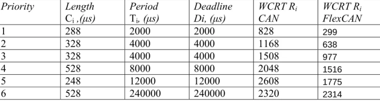
Table , shows the results of WCRT calculations for CAN and FlexCAN, using the same set of messages as that in [] for a data rate R of 250 Kbps and assuming no errors (i.e., K = 0). It can be noticed that the bound of the FlexCAN calculations are much more tighter than that for the case of CAN.

Table . Comparison of worst case response time (WCRT) results for CAN and FlexCAN for a typical set of 6 messages of varying lengths, R = 250 Kbps.

Priority Length Ci ,(μs) Period Ti, (μs) Deadline Di, (μs) WCRT Ri CAN WCRT Ri FlexCAN 1 288 2000 2000 828 299 2 328 4000 4000 1168 638 3 328 4000 4000 1508 977 4 528 8000 8000 2048 1516 5 248 12000 12000 2608 1775 6 528 240000 240000 2320 2314

Calculating message response times in FlexCAN has the following advantages:

1. The calculations are more accurate since they are done on a sub-cycle basis relative to a time-triggered communication cycle with each sub-cycle being independent from the next (i.e., all messages are sent in their respective sub-cycles)

2. The calculations are easy to evaluate as the equations are not in closed-form and

furthermore both Ii(ti) and Ei(ti) do not depend on ti.

3. The formulae assume that the jitter Ji is zero which is enforced by the FlexCAN

message schedule.

4. The formulae are accurate because the term Bm = S, (i.e., there is no uncertainty

regarding Bm).

5. The multi-rate case is taken into account ahead of time by the FlexCAN message global schedule thus the various periods T1, T2, … do not appear explicitly in the

equations.

In summary, note the following properties of FlexCAN,

1. It is a TT system with communication cycles and sub-cycles.

2. It is a sub-network where messages do not have widely varying transmission periods

Ti.

3. An off-line global message schedule takes care of the multi-rate case. 4. Message latency calculations are done per sub-cycle

) ( ) ( S C I _j i hp j i =

∑

5. All messages scheduled in a sub-cycle are submitted for transmission at exactly the same time (at the beginning of the sub-cycle).

6. All messages in a sub-cycle have the same deadlines Di= Tsc.

Solution of the Problem

Going back to the problem of finding the probability of failure delivery of message mi,

Pmerr = Prob. (Ri > Tsc), we start by using the notation p(Ri/K) to represent the upper bound

on the probability that a frame is affected by exactly K faults and hence may arrive no later than Ri/K, that is,

p(Ri/K) = Prob { Ri/K < Tsc }

Broster et. al. [] have provided a solution for finding Pmerr which is slightly modified

here for the case of FlexCAN, where Di = Tsc, and the periods Ti are all the same in the

sub-cycle in question1.

Pmerr = Prob {Ri/K > Tsc}

= 1 -

∑

R

p

)

(

Where p(Ri/n) is computed recursively as follows,

p(Ri/n) = p(n, Ri/n) -

∑

p(Ri/j) p(n-j, Ri/n - Ri/j)

Numerical Results

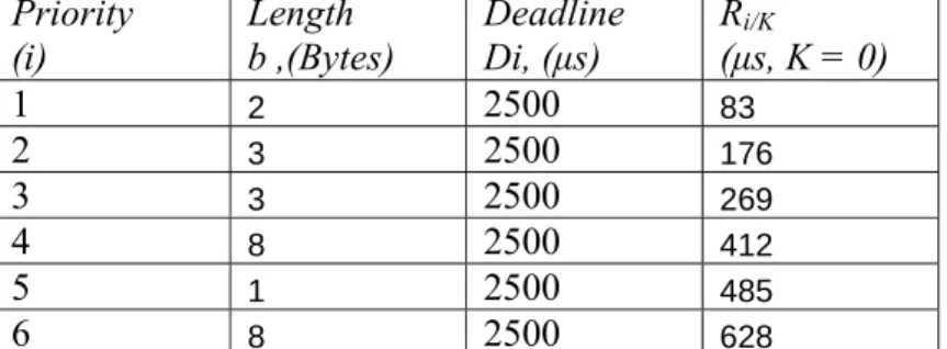
Table . Worst case response time (WCRT) for a FlexCAN schedule with Tsc = 2.5 msec,

a set of 6 messages of varying lengths, R = 1 Mbps, and K = 0.

Priority (i) Length b ,(Bytes) Deadline Di, (μs) Ri/K (μs, K = 0) 1 2 2500 83 2 3 2500 176 3 3 2500 269 4 8 2500 412 5 1 2500 485 6 8 2500 628

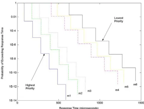
The results of the FlexCAN probabilistic analysis for R= 1 Mbps with λ = 30

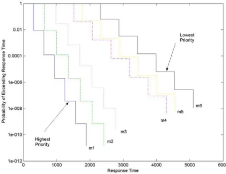
faults/second appears in Figure A as a cumulative probability distribution. The graph shows the probabilities of each message exceeding a given response time. Fig. B shows the probabilities as a function of message priorities with the message response time as a parameter. Figures C and D are likewise but for a data rate R of 250 Kbps.

1 _{The deadlines and transmission periods correspond to messages already scheduled on a sub-cycle. They} may be different to the deadlines and transmission periods of the entire set of messages. It should be noted that a multi-rate case has already taken into account by the scheduling process.

Figure A. Worst case probability of exceeding a response time for six messages arranged in priority order (R = 1 Mbps).

Figure B. Worst case probability of exceeding a response time as a function of message priority. Priority 1 is the highest priority (R = 1 Mbps).

Figure C. Worst case probability of exceeding a response time for six messages arranged in priority order (R = 250 Kbps).

Figure D. Worst case probability of exceeding a response time as a function of message priority. Priority 1 is the highest priority (R = 250 Kbps).

Further FlexCAN Properties

1. Successful transmission of message mi implies successful transmission of messages mk, where k < i.

2. The worst case response time Rk < Ri , for k < i.

3. Rk/K < Ri/K, for k < i, ∀ K

4. For a fixed response time R, p(Rk/n) < p(Ri/j) , for k < i, such that Rk/n = Ri/j = R, ∀

n,j.

5. For a fixed probability level P, Rk/n > Ri/j, for k < i, such that p(Rk/n) = p(Ri/j) = P,

∀ n,j. Conclusions

• Message latency calculations for FlexCAN are much simpler than those for CAN. • Several graphs were generated that are useful for sizing, dimensioning, and

configuring FlexCAN networks for specific applications.

• Just like CAN, FlexCAN outperforms TT-CAN and TDMA networks for transient random failures.

• FlexCAN retains most of the error recovery properties of CAN at the expense of a smaller bandwidth utilization.