HAL Id: hal-00326956
https://hal.archives-ouvertes.fr/hal-00326956
Preprint submitted on 6 Oct 2008
HAL is a multi-disciplinary open access
archive for the deposit and dissemination of
sci-entific research documents, whether they are
pub-lished or not. The documents may come from
teaching and research institutions in France or
abroad, or from public or private research centers.
L’archive ouverte pluridisciplinaire HAL, est
destinée au dépôt et à la diffusion de documents
scientifiques de niveau recherche, publiés ou non,
émanant des établissements d’enseignement et de
recherche français ou étrangers, des laboratoires
publics ou privés.
carbon interacting with transition metals: Application
to the Ni-C system
Hakim Amara, Jean-Marc Roussel, Christophe Bichara, Jean-Pierre Gaspard,
François Ducastelle
To cite this version:
Hakim Amara, Jean-Marc Roussel, Christophe Bichara, Jean-Pierre Gaspard, François Ducastelle. A
tight-binding potential for atomistic simulations of carbon interacting with transition metals:
Appli-cation to the Ni-C system. 2008. �hal-00326956�
transition metals: Application to the Ni-C system
H. Amara,1 J.-M. Roussel,2 C. Bichara,3 J.-P. Gaspard,4 and F. Ducastelle5
1DSM/IRAMIS/SPAM/Laboratoire Francis Perrin, CEA Saclay,
Bˆatiment 522, 91191 Gif sur Yvette Cedex France
2Universit´e Aix-Marseille, IM2NP, UMR CNRS 6242, Case 142,
Facult´e des Sciences de St-J´erˆome, 13397 Marseille Cedex 20, France
3Centre Interdisciplinaire de Nanosciences de Marseille, (CINaM),
UPR CNRS 3118, Campus de Luminy, case 913, 13288 Marseille Cedex 09, France
4Institut de Physique, Universit´e de Li`ege, 4000 Sart-Tilman, Belgique
5Laboratoire d’Etudes des Microstructures, ONERA-CNRS, BP 72, 92322 Chˆatillon Cedex, France
(Dated: October 6, 2008)
We present a tight-binding potential for transition metals, carbon, and transition metal carbides, which has been optimized through a systematic fitting procedure. A minimal basis, including the s, p electrons of carbon and the d electrons of the transition metal, is used to obtain a transferable tight-binding model of the carbon-carbon, metal-metal and metal-carbon interactions applicable to binary systems. The Ni-C system is more specifically discussed. The successful validation of the potential for different atomic configurations indicates a good transferability of the model and makes it a good choice for atomistic simulations sampling a large configuration space. This approach appears to be very efficient to describe interactions in systems containing carbon and transition metal elements.
PACS numbers: 61.50.Lt,61.72.Bb,71.15.Nc,71.20.Be,81.05.Je
I. INTRODUCTION
Carbon-metal interactions play a major role in many aspects of materials sciences, in particular when transi-tion metals are involved. They lead to the formatransi-tion of solid solutions or of compounds in which carbon occu-pies interstitial sites. Early transition metals (Ti, V, Cr, Zr, Nb, Mo, Ta, for instance) have a tendency to form highly stable carbides whereas such carbides are hardly stable (cementite Fe3C) or metastable (Ni3C, Co3C) in
the case of Fe, Co and Ni.1The phase diagrams involving
the latter elements present broad domains of two-phase mixtures. The domains of stability of solid solutions are narrow, but of outmost importance (steels).
These elements, as well as some other elements of the ends of the transition series (Pd, Pt), are also well known for their catalytic properties involving the chemistry of molecules containing carbon. The oxidation of carbon monoxide on transition metal surfaces is for example one of the most extensively studied heterogeneous catalytic reactions in relation with the air pollution problem. Sur-face reactions of methane on nickel surSur-faces have also been investigated extensively, since they are involved in industrial reactions, such as steam reforming of methane and methanation of carbon monoxide.2
Another more recent example of the catalytic impor-tance of these elements which has motivated this work is the catalytic growth of carbon nanotubes (CNT). CNT have remarkable physical properties with the potential for significant technological impact. In many applica-tions, optimal performance requires the control of their structural properties, e. g. size, length and chirality, which remains a significant difficulty for the widespread
application of carbon nanotubes in high-technology de-vices. Unlike the case of multi-wall nanotubes (MWNT), the formation of single-wall carbon nanotubes (SWNT) requires the presence of transition metal element or alloy catalysts (Co, Ni, Fe, Y,. . . ).3,4,5SWNT are synthesized
via the interaction of metal-catalyst nanoparticles with carbon or hydrocarbon vapours at relatively high tem-perature. These catalysts are crucial for the controlled synthesis of SWNT, by different techniques such as laser ablation,6 arc discharge method3 or chemical vapor
de-position.7,8,9However, the exact role played by the metal
atoms in the growth of SWNT is still under study.10
Many theoretical works have been devoted to the in-vestigation of the unique properties of transition metal carbides in connection with their electronic structure and bonding characteristics. Most of these works are based on static ab initio calculations.11 However, understanding
the nucleation and growth mechanisms involved in cat-alytic processes and validating them by computer simula-tions requires to model fairly complex processes involving strong modifications of the bonding between carbon and the transition metal atoms. For example the catalytic growth of SWNT involves segregation and diffusion pro-cesses of carbon atoms and the self-organization of these atoms into graphene sheets and nanotube embryos close to the catalytic surface.
A challenge for such simulations is to have an energy model able to describe the competition between very dif-ferent carbon environments. In the case of solid solutions or of ordered compounds, metal–C bonds are predomi-nant around C atoms. When phase separation occurs, carbon atoms have to segregate to form pure graphite or metastable, more or less well crystallized, phases of
bon, in which case carbon atoms form covalent sp2, sp3
or even sp bonds. These processes can only be sim-ulated using large enough systems (hundreds or thou-sands of atoms) during fairly long times, typically in the range 10−9s – 10−6s. Ab initio molecular dynamics
calculations4,12 cannot therefore be used systematically
at such size and time scales. On the other hand, us-ing simple phenomenological potentials13in different
sit-uations is problematic — the transferability problem — since such potentials can hardly account for the (quan-tum) nature of the different types of covalent bonds.
The aim of this paper is to present and discuss the va-lidity of a simple intermediate model for carbon and tran-sition metal interactions based on a tight-binding descrip-tion of the chemical bonds. Applicadescrip-tions of this model to surface segregation of carbon and to the catalytic nucle-ation of carbon caps on small nickel clusters have already been presented elsewhere.10,14,15,16 Although the model
can be extended to all transition elements, we concen-trate here on fcc metals and more particularly on nickel. The paper is organized as follows: In Sec. II, we present the tight-binding model and the recursion technique used to calculate band energies. Empirical repulsive contri-butions are then added to obtain total energies. Sec-tions III and IV describe the corresponding models for the carbon-carbon and nickel-nickel interactions, respec-tively, whereas Sec. V is devoted to a discussion of the electronic structure of transition metal carbides and of nickel-carbon interactions. Different validations and ap-plications of the model are finally developed and dis-cussed in Sec. VI.
II. METHODOLOGY
When using the tight-binding (or extended H¨uckel) approximation, the first step is to define a basis set of atomic orbitals. To describe the valence states of car-bon, the set must of course include the 2s and 2p states. In the case of the transition elements, d states must also be included, the problem being to decide whether s and p states of the metallic element should be kept also. Since we are interested in cohesive energies more than in a de-tailed description of the electronic structure, we have cho-sen to use the simplest basis where the contribution of these states is neglected. When interested in more de-tailed electronic structure properties, sp − d hybridiza-tion should however be taken into account and this can be done, as shown for example by Barreteau et al.17
An-other more complete, but much heavier to implement, tight-binding scheme has also been derived by Andriotis et al. (see Ref. [18], and references therein).
Thus, we will work with the following basis |i, λi where i denotes the lattice sites and λ denotes the orbital index, (λ = s, px, py, pz, dxy, dyz, dzx, dx2−y2, d3z2−r2).
As usual in the simplest tight-binding approximation, we neglect the direct overlap integrals hi, λ|j, µi = δijδλµ
and the three-central integrals. We are then left with the
usual hopping or (transfer) integrals β defined in terms of the interatomic matrix elements of the hamiltonian H:
βiλ,jµ = Hiλ,jµ = hi, λ|H|j, µi ; i 6= j , (1)
which are responsible for the broadening of the discrete atomic levels into energy bands. They are functions of the direction cosines l, m, n of ~rij = ~rj − ~ri and of a
limited number of parameters, the Slater-Koster param-eters,19which decrease rapidly with the interatomic
dis-tance rij. Since the atomic potential is assumed to be
spherically symmetric, the (9 × 9) matrix of hopping in-tegrals between sites i and j is completely determined by ten Slater-Koster hopping parameters (ssσ, spσ, ppσ, ppπ, ddσ, ddπ, ddδ, sdσ, pdσ, pdπ). The intra-atomic matrix elements of the hamiltonian H are given by:
Hiλ,iµ = (εiλ+ αiλ,jλ)δλµ , (2)
where εiλ is the atomic level of the orbital |i, λi. The
second term in the right hand side of Eq. (2) is a so-called crystal field integral which determines the displacement of the average energy level. This shift is neglected here. In the case of a transition metal carbide, three atomic levels have to be determined, i. e. εs, εp for carbon and
εdfor the transition metal atom.
As usual in such a semi-phenomenological tight-binding scheme, we assume that the total energy (com-pared to the energy of the free atoms) Etotcan be written
as the sum of a band structure, attractive, contribution which describes the formation of an energy band when atoms are put together and of a phenomenological repul-sive term which empirically accounts for the ionic and electronic repulsions.20,21,22 It is convenient to
decom-pose these terms into local contributions Ei
band, Eirepand
Ei tot, so that: Etot= X i atoms Ei
tot ; Etoti = Ebandi + Erepi . (3)
The band energy, Ei
band, is given by:
Ei band =
Z EF −∞
(E − εi)ni(E)dE , (4)
where EF denotes the Fermi level, εiis the atomic energy
level introduced previously and ni(E) is the local density
of states (LDOS). To define and calculate this LDOS, we first define the Green function (or resolvent), G(z):
G(z) = (z − H)−1 . (5)
The total density of states per atom n(E) = (2/N )Pnδ(E − En), where the factor 2 takes into
ac-count the spin degeneracy, and N is the number of atoms, is related to the trace of the Green function through:
n(E) = − 2
πN ε→0lim+Im Tr G(z) . (6)
Projecting G(z) on the orbital |i, λi, we obtain the local density of states niλ(E) on site i and for orbital λ:
ni,λ(E) = −
2
πε→0lim+ImGiλ,iλ(z) , (7) where Giλ,iλ(z) is the diagonal element of the Green
func-tion. The LDOS ni(E) is then given by:
ni(E) =
X
λ
ni,λ(E) , (8)
so that, obviously, n(E) = (1/N )Pini(E). Notice here
that, using the properties of the resolvent, a decomposi-tion of the band energy into bond energies rather than into site energies can be derived, which can be conve-nient in some cases. This has been discussed in detail by Pettifor et al.; see Ref.[23] and references therein.
We now use the recursion method24 to calculate the
local density of states niλ(E) and more precisely the
con-tinued fraction expansion of Giλ,iλ(z):
Giλ,iλ(z) = 1 z − aiλ 1 − (biλ 1 )2 . .. z − aiλ M − (biλM)2ΣM(z) , (9)
where the coefficients (a, b), which are related to the moments of the density of states, are obtained from the recursion procedure, and where ΣM(z) is the tail
of the continued fraction. As compared to the stan-dard diagonalization technique, we make here two addi-tional approximations: only the first moments are calcu-lated exactly for the considered atomic structures, which means that only a few coefficients (a, b) are calculated exactly.25Many constant coefficients up to the Mthlevel
are then inserted, after what the continued fraction is cut, ΣM(z) = 0. Giλ,iλ(z) can then be written as the
ratio of two polynomials and finally the local density of states ni(E) is obtained as a set of M delta-functions at
positions (Eij, j = 1, M ) and weights (Aji, j = 1, M ) by diagonalizing a tridiagonal matrix of size M . This ap-proach, of order N , is particularly useful for the study of large and fully relaxed systems. It corresponds to em-bedding site i and its local atomic environment within an effective medium. In principle the Fermi level is fixed by a global neutrality condition, Ne=
REF
−∞n(E)dE so that,
in general, the local charges Ni e =
REF
−∞ni(E)dE differ
from Ne. In metallic systems the usual rule is to impose
a local charge neutrality condition, which can be done by introducing local variations of the atomic energy levels. This insures to some extent the validity of the decom-position (3) of the total energy.21,26 More precisely the
variational properties of the ground state energy insures that, even if charge transfers occur, the ground state en-ergy can be calculated to lowest order as if charge trans-fers are neglected. Instead of varying the energy levels, a more approximate but much easier procedure is to intro-duce fictitious local Fermi levels, so that finally the local
energy can be written:
Ei tot= jXmax j=1 Ai jEji , (10)
where the highest occupied energy level jmaxdepends on
each site i and is simply determined through the local neutrality conditionPjmax
j=1 Aij= Ne.
III. CARBON
Because of the technological importance of carbon, a large number of “potentials” has been proposed in the literature to modelize its cohesive properties. We adopt here the usual term “potential” to describe a model al-lowing us to calculate the total energy of a system for any positions of the atoms considered as classical vari-ables. A first class of potentials has been derived by Stillinger and Weber27 and by Tersoff;28 they are based
on a pairwise additive description of the total energy, sup-plemented by angular terms to take into account the di-rectional spncovalent bonding of carbon. Such terms are
actually necessary to insure the stability of non-compact atomic structures, i. e. structures with low coordination numbers.
Among the more recent developments, we can men-tion the formulamen-tion in terms of bond order,23 the
in-clusion of dependences on the environment29 as well as
potentials allowing to treat both carbon and hydrocar-bon phases.30,31For a recent discussion, see e. g. Ref.[32].
The accuracy of such potentials depends critically on the validity of the data base to which the parameters are fit-ted. Improving the accuracy usually implies increasing the number of parameters, which can blur the physical transparency of the model and leaves the question of the transferability unresolved. The main reason for their suc-cess is their low computational cost that makes large scale computations of thousands of atoms affordable.
A second popular class of potentials has been derived in the framework of a tight-binding approximation which is indeed well known to provide very good descriptions of the electronic structure and of the energies of carbon covalent bonds. Following a parametrization of the tight-binding hamiltonian by Goodwin et al.33 for silicon, Xu
et al.34proposed an interaction model for carbon that has
been widely used. Improvements over this relatively sim-ple model include three-center integrals and environment dependent parameters for the hopping integrals and the repulsive term.35Although in principle more transferable
than empirical models, the tight-binding models also de-pend on adjustable parameters to build the hamiltonian matrix of the interactions and to describe the empirical repulsive term that is always present. These parameters are usually fitted to ab initio or experimental data, al-though Porezag et al. used a density functional-based scheme to determine the parameters of a non-orthogonal tight-binding model.36
In our model, we start from the potential of Xu et al.34 to describe the band structure term, but instead of
performing a diagonalization of the hamiltonian matrix, we consider local densities of states ni(E). Both s and p
electrons are taken into account, with the corresponding s, px, pyand pzatomic orbitals. To calculate the cohesive
energy of the system, we assume the same atomic energy levels for C (εs = −2.99 eV and εp = 3.71 eV, but the
model only depends in fact on the difference εp−εs= 6.70
eV), and the same dependence on distance of the hopping integrals as that given by Xu et al.:34
βλ(r) = βλ0(r0/r)nexp{n[−(r/rc)nc+ (r0/rc)nc]} . (11)
The values of β0
λ corresponding to the different
interac-tions at the diamond interatomic distance r0 = 1.536
˚
A, are given by β0
ssσ = −5.00 eV, β0spσ = 4.70 eV,
β0
ppσ = 5.50 eV and β0ppπ= −1.55 eV.
The coefficients of equation (11) are n = 2.00, nc =
6.50, and rc = 2.18 ˚A. As explained in Sec. II, only a
few continued fraction coefficients are calculated. We keep only four coefficients (a1, b1, a2, b2) which
corre-sponds to a fourth moment approximation, i. e. the first four moments of the local density of states ni,λ(E) are
calculated exactly on each site of the considered atomic structure. This is the minimal approximation that takes into account the directional character of the carbon s − p bonds. The local density of states ni(E) on site i then
only depends on the first and second neighbours of i, a neighbour being defined here as an atom closer to i than a given cut-off distance. The cut-off distance for car-bon is fixed at 2.70 ˚A. To restore rotational invariance, a problem that plagues the use of the recursion method in the case of p-bonded systems,37 we proceed as
fol-lows: unlike the coefficients, the moments of the LDOS are linear functionals of these LDOS; they can therefore be averaged over the p orbital index; then new coeffi-cients corresponding to the p LDOS can be calculated. As explained in Sec. II, the related continued fraction is then expanded up to the Mth level using constant
co-efficients equal to a2 and b2. A typical value for M is
M = 40. High enough values are necessary to obtain quasi-continuous densities of states.
For the repulsive part of the energy we use also the form proposed by Xu et al.34 but the parameters had to
be modified for the following reason. Although fairly ac-curate, the energies calculated within our fourth moment approximation are not exactly equal to those determined after a full diagonalization procedure. Since it is impor-tant to have a model that reproduces accurately the com-petition between the different crystalline forms of carbon, and more importantly, the competition between graphite and diamond, new fits should be performed. The repul-sive energy has the form:
Ei rep= F (
X
j6=i
φ(rij)), (12)
where F (x) is a polynomial function :
F (x) = C1x + C2x2+ C3x3+ C4x4+ C5x5 (13)
and φ(rij) is a repulsive pairwise potential
φ(r) = φ0(d0/r)mexp{m[−(r/dc)mc+ (d0/dc)mc]} (14)
The parameters were fitted using a a Levenberg-Marquardt method38 to match the total energy curves
of selected structures obtained using ab initio FPLMTO calculations (WIEN97 code39). These structures include
a C3 linear molecule, an infinite linear chain, a graphene
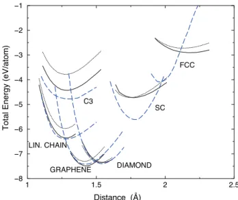
sheet, diamond, simple cubic and face centered cubic lat-tices. Fig. 1 presents the total energy curves as a function of the nearest neighbour distance for the various struc-tures used for the fit. Both LDA and GGA calculations were performed and the ab initio results were shifted to the experimental energy for diamond at its equilibrium distance (Etot= −7.34 eV/atom at d = 1.53 ˚A). The
pa-rameters were fitted to the GGA values with more weight on the linear chain, graphene and diamond structures. The total energy curves match very well the ab initio
re-1 1.5 2 2.5 Distance (Å) −8 −7 −6 −5 −4 −3 −2 −1
Total Energy (eV/atom)
FCC SC DIAMOND GRAPHENE LIN. CHAIN C3
FIG. 1: Total energy as a function of the interatomic dis-tance for C3, linear chain, graphene, diamond, simple cubic
and face centered cubic structures. Thin dotted line: LDA approximation; full line: GGA approximation; thick dashed line: 4th
moment approximation.
sults for carbon in its sp, sp2and sp3bonding states. The
molecules and the simple cubic and fcc phases are too sta-ble as compared to the ab initio results but still far from being stable. Finally, the coefficients in Eq. (13) are given by: C1 = 6.2148, C2 = −0.48797, C3 = 0.50716.10−1,
C4 = −0.28906.10−2, C5 = 0.69083.10−4. The
co-efficients in Eq.(14) are: φ0 = 1.3572, d0 = 1.5096,
m = −3.4528, dc = 2.0798, mc = 7.0584.
Further-more, to avoid any discontinuity in the energy calcula-tions, Fermi-like cut-off functions are used. In Eq.(11), the βλ(r) are replaced by βλ(r)/[1 + exp((r − δ1)/σ1)]
with δ1= 2.53˚A and σ1= 0.016˚A, while in Eq.(14), φ(r)
is changed into φ(r)/[1 + exp((r − δ2)/σ2)] with δ2= 2.59
˚
A and σ2= 0.0033 ˚A.
A reliable model to study the synthesis of carbon nanostructures should not only yield the correct relative
energies for carbon in its sp, sp2and sp3 states but also
correct energy barriers between these states. Kertesz and Hoffman40, and Fahy et al.41 have calculated the energy
barrier corresponding to the transition from rhombohe-dral graphene to diamond. Following the same path in the R (bond length between layers), θ (buckling angle) and B (bond length within layers) space, we find the same value ∆E = 0.33 eV/atom as in Ref.[41] for slightly different values of the parameters (see Fig. 2).
FIG. 2: Total energy difference for the diamond to rhombo-hedral graphite transition along the path in the R, θ, B space defined in Ref. [41]. Circles: 4th
moment approximation; di-amonds: Fahy et al.41
Finally, we study typical defects that are likely to oc-cur in sp2 carbon nanostructures, such as adatoms and
Stone-Wales defects. Since a carbon adatom is a common defect in graphitic lattices, it is important to study its behaviour within our model. Using a simulated anneal-ing procedure, we find that the equilibrium position of the adatom corresponds to a bridge-like structure where the adatom lies above a C–C bond. This geometry and the energy gain (equal to -0.93 eV) are similar to those obtained within previous LDA calculations on a similar surface.42,43,44 This result is a priori far from obvious
since it could have been imagined that a “hole” position where the atom lies above the centre of an hexagon is more favourable. This is therefore a very nice validation of the potential. The distance of the adatom perpendic-ular to the graphene plane is equal to 1.25 ˚A with C–C bond length equal to 1.42 ˚A and bond angle close to 98◦.
The Stone-Wales defect is a 90◦ rotation of two
car-bon atoms in the hexagonal network with respect to the midpoint of the bond. This leads to the formation of two pentagons and two heptagons, replacing four hexagons.45
This transformation, studied extensively theoretically us-ing first-principles calculations, has been shown to give rise to extremely high-energy barriers of 6 to 10 eV with an energy of formation around 4–5 eV.46Our
tight-binding model yields reasonable values with an energy barrier equal to 7.2 eV and an energy of formation equal to 6.0 eV. Notice that the presence of adatoms
consider-ably lowers the energy barrier.47
IV. TRANSITION METAL
The electronic structure of transition metals is charac-terized by the presence of tightly bound d electrons which form a narrow band that overlaps and hybridizes with a broader nearly-free-electron sp band, and most physical properties of these metals have a systematic variation across the transition-metal series, as a function of the number of valence d electrons. This is well described within the tight-binding approximation21,22,48where
sp-d hybrisp-dizations are neglectesp-d ansp-d in which the mean position of the d band in the solid is assumed to be given by the atomic level εd. In particular, the bell shape
be-haviour of the cohesive energy and of the elastic moduli is correctly predicted by these models and is the result of a progressive filling of the d states.20 In our d band
model, the Slater-Koster parameters for the hopping in-tegrals ddσ, ddπ and ddδ are assumed to be in the ratios −2 : 1 : 0 and to decay exponentially with respect to the bond length r as:
ddλ(r) = ddλ0exp[−q(r/r0− 1)] , (15)
with λ = σ, π, δ. The second term in Eq.(3), Ei rep, is a
repulsive contribution, chosen to have a pairwise Born-Mayer form here:
Erepi = A X j atoms exp[−p(rij r0 − 1)] . (16)
The (ddλ0, q, A, p) parameters used in this study are
fitted to experimental values of the lattice parameter, of the cohesive energy, and of the elastic moduli (bulk mod-ulus and the two shear moduli) for the fcc elements at the end of the 3d transition metal series, cobalt and nickel. Both elements have quite similar cohesive properties, as shown in table I. In practice the procedure is to force almost perfect agreement with the experimental data for the lattice parameter, cohesive energy, and bulk modu-lus and to find a good compromise for the shear moduli. There are however well-known problems with the treat-ment of the late transition eletreat-ments using a pure d tight-binding approximation. The main difficulty is that the calculated shear moduli for the fcc structure C = C44
and C′ = (C
11− C12)/2 are negative for a d band
fill-ing Nd larger than 9, which is the usual value chosen for
Ni, Pd, Pt.52The fcc lattice is then completely unstable,
and actually the bcc structure is found to be more sta-ble for nearly filled d bands, when performing total en-ergy calculations.53,54,55 Similarly the cohesive energies
are much too low.
All these disadvantages are known to be due to ne-glecting hybridization of the d states with the nearly free electron states built from the s and p atomic states. Un-fortunately adding s and p states to the atomic basis multiplies the number of parameters to be fitted, so that
TABLE I: Comparison of our tight-binding d model with experimental data. The experimental values for fcc Ni and hcp Co are taken from Ref.[49]; those for fcc Co from Ref.[50] and the surface energies from Ref.[51].
Structure Lattice Cohesive B C′ C
44 Surface
parameter energy energy
˚
A eV/at GPa GPa GPa mJ/m2
Ni fcc a/√2 = 2.489 -4.44 187.6 55.2 131.7 1840 (solid) 2385 (liquid) Co hcp a=2.50 -4.39 193 1884 (liquid) c=4.07 Co fcc 182 32.5 92 This work fcc a/√2 = 2.489 -4.44 182.1 68.8 96.9 1660 (100) 1560 (111)
the model becomes fairly complicate, if not unstable. We have checked that the fourth moment approximation that we use here as in the case of carbon (Sec. III) reproduced fairly well the results obtained from a full diagonalization of the tight-binding hamiltonian for d band fillings close to 8. For this band filling which turns out to be in be-tween the values recommended by Andersen for Co and Ni,56the fit to the experimental values is fairly good (see
Table I) and stable. We have therefore chosen this value, which will be used for nickel in the following. It could be applied to cobalt as well: our model is too simple to discriminate between these two elements.
Let us recall here, that paradoxically a second mo-ment approximation would provide positive shear mod-uli, which explains why it is used with success in some cases. But this is clearly an artifact. Since we want to have a consistent and simple scheme to describe cor-rectly the sp states of carbon and the d states of the transition elements, the fourth moment approximation is a good compromise. A fifth or sixth moment approxi-mation would be better still52,57 but fairly expensive to
implement.
Within the fourth moment approximation described previously, the parameters are ddπ0= 0.54 eV, r0= 2.53
˚
A, q = 2.14, A = 0.0795 eV and p = 12.1. Here again, the hopping integrals ddλ and the repulsive interactions are forced to vanish smoothly using a Fermi-like function, 1/(1 + exp[(r − δ3)/σ3), where δ3= 2.95 ˚A and σ3= 0.08
˚
A. There are of course more sophisticated methods to optimize the dependence on distance of the hopping in-tegrals. Actually it is not possible in all cases to obtain reasonable fits using a single smooth law for this depen-dence. For example first and second neighbour integrals on a bcc lattice do not obey similar laws. This can be accounted for by defining “screened” integrals depending on the local environment.58 In the case of the fcc
struc-tures considered here, this is not necessary.
V. METAL-CARBON INTERACTIONS
To describe the carbon-metal interactions, it is very convenient to start from a study of the electronic
struc-ture of simple and typical metal carbides. The tran-sition metal compounds of type MX (M = 3d transi-tion metal, X =C and N) have attracted much attentransi-tion due to their remarkable mechanical and physical proper-ties, e. g., high hardness, high melting points, and wear and corrosion resistance.59 Most of the transition metal
monocarbides crystallize in the NaCl structure, where carbon atoms occupy the octahedral interstitial sites of the fcc metallic sublattice. This concerns principally the elements of groups IV (Ti, Zr, Hf) and V (V, Nb, Ta). In-creasing the number of d electrons stabilizes an hexagonal structure where the octahedral sites are replaced by trig-onal prismatic sites (case of MoC and WC for example). Many other interstitial transition carbides form at dif-ferent stoichiometries.1Another large family of carbides
and nitrides can be viewed as resulting from the ordering of vacancies on the carbon (nitrogen) sublattice.60These
ordering mechanisms have been well explained from the calculation of effective pair interactions within a tight-binding model.21,61
The relation between the cohesive properties of tran-sition metal compounds and their electronic structure is a matter of considerable theoretical and practical in-terest.11 In particular, band structure calculations have
been performed very early for the MX NaCl-like com-pounds62,63 and their main physical conclusions have
been confirmed by self-consistent LDA calculations.64,65
Extensive compilations of thermodynamic data and of electronic structure calculations of cohesive properties are available.66,67
All these works show that the cohesive properties of the MX carbides can be understood in a model similar to the Friedel model for transition elements, where the cohesive energy varies with the filling of a valence band built here from hybridized pd states. In a first approxi-mation a rigid band model is valid, the density of states of carbides being characterized by the presence of a fairly broad band of strongly hybridized states between the p states of carbon and the metallic d states.
More precisely the electronic structure of a typical NaCl carbide is characterized by three families of states (see Fig. 3). The calculations presented in this figure have been performed using the ABINIT code;68 see also the
data base of D. Papaconstantopoulos.69 At low-energy
(typically 10 eV below the Fermi level) there is a narrow band derived from the 2s states of carbon. At higher en-ergy appears the hybridized pd band with a pseudo-gap within it, separating bonding states from anti-bonding states. Notice that the cubic symmetry allows us to dis-tinguish between eg and t2g states, and that the pd
hy-bridization is found to be more efficient for eg states.
Fi-nally at much higher energy, about 9 eV above the pseu-dogap, there is a nearly free electron band built princi-pally from the s and p states of the metallic element. The electronic structure of NaCl nitrides is quite similar, with a deeper pseudogap. Finally in the case of oxides, a gen-uine gap appears and these oxides are insulators whereas the carbides and nitrides are metallic. All these features are fairly well understood and are typical of interstitial compounds where the interstitial elements (carbon, ni-trogen, oxygen) do not interact directly.11 The shortest
interatomic distance is the carbon (nitrogen, oxygen) – metal distance, hence the strong pd hybridization.
On the other hand the interstitial-interstitial distance is much larger in a fcc lattice than in the correspond-ing molecules C2, N2, O2 and the s and p states of the
interstitial atom do not hybridize. Actually the 2s low energy band practically does not play any role in bond-ing. From this discussion it is clear that a tight-binding fit of the energy bands of NaCl carbides should be fea-sible, and this has been achieved indeed in a pioneering work by Schwarz on NbC62 whose electronic structure is
quite similar to that of TiC. This type of fit combined with the recursion method has been used with success afterwards70 and will serve here as a reference. We can
even simplify this description by neglecting crystalline field integrals, as well as the sdσ integrals coupling the carbon s states and the transition d states, because of their weak interactions mentioned above. Finally in this simplest scheme, the electronic structure of all transition NaCl carbides can be characterized by three parameters, the two hopping integrals pdσ and pdπ and the position of the d states εd compared to that of the carbon s and p
states, εsand εp. The hopping integrals are also assumed
to decay exponentially with distance:
pdλ(r) = pdλ0exp[−q(
r r0
− 1)] ; λ = σ, π . (17)
Using the following values: pdσ = −2.319 eV, pdπ = 1.306 eV, r0 = 1.88 ˚A, we have checked that this model
is sufficient to reproduce the main characteristics of the density of states of NbC corresponding to the valence pd band (see Fig. 4). The fact that the lowest 2s band is not very well treated is not important here as discussed above. The parameter q will be also determined later on.
Let us now discuss a few problems related to the elec-tronic populations and charge transfers. When looking at the band structure of a typical NaCl carbide (see Fig. 3) we see that the lowest s band contains one state per unit cell (or per formula MC), and therefore two states,
FIG. 3: Top: band structure and density of states of the TiC carbide: the Fermi level (dashed line) is just in the middle of the pseudogap within the hybridized pd band. Bottom: partial s, p and d densities of states. The calculations are made with the ABINIT code.68
spin included, per formula. The set of sp bands above contains eight bands, hence sixteen states per formula. Within our model these states are built from the six p states of carbon and the ten d states of the metallic ele-ment. This means that the states built from the sp states of this element contribute to the states at higher energy, abovethe main pd hybridized band. The nearly free elec-tron band does not overlap the d states, whereas we know that such an overlap occurs in elemental transition ele-ments. Actually the interactions between the s states of carbon and the sp states of the metallic element repel the latter states above the main hybridized band. There is a charge transfer from sp states towards d states when going from the pure element to the carbide. Since we do not include the metallic sp states in our basis, we have just to change the d population. As an example, consider the TiC compound. The valence charge of Ti is equal to
n(E) (arb. units) -15 -10 -5 0 5 Energy (eV) 0 5 10 15 20
FIG. 4: Comparison between the density of states of NbC corresponding to the full fit by Schwarz62
(dashed line) and that obtained within our simplified scheme. The agreement is good as far as the relevant valence bands are concerned.
4. In the case of the carbide we have therefore to fill the hybridized pd band with 4+ 2 (carbon p electrons) elec-trons. For pure titanium it is generally considered that the d band filling is about 3, which corresponds to an effective d3s atomic configuration instead of d4 for the
carbide. Since the band energy varies quite a lot with the effective number of d electrons, this effect cannot be neglected. Viewed from the side of the metallic atom, all happens as if the presence of carbon atoms on the oc-tahedron sites of its first neighbour shell has induced a transfer of one electron from the (metallic) sp states to the d states. To build a potential for any atomic config-uration we adopt an interpolation procedure where the number of electrons transferred is a smooth function of the number of carbon atoms (between zero and six) on the first coordination shell. Beyond six carbon atoms this number is held constant.
Although NaCl carbides do not exist in the case of Fe, Co, and Ni, we can rely on the first principles calcu-lations which indicate that the shape of the hybridized band does not change too much when varying the element of the transition series (see Fig. 5). We will therefore keep the values of the hopping integrals derived for NbC. The position of the atomic d level on the other hand obviously varies with the nature of the element considered. εd
de-creases when increasing the number of electrons along a transition series (about 1 eV per element), but since this level is an effective quantity, which is adjustable to some extent, it is useful to see how it is related to the charge transfers between carbon and the metallic element.
Within the tight-binding method one uses so-called Mulliken charges which are based on the decomposition of the electronic density on the atomic orbitals. Here, they are obtained by integrating the local densities of
-15 -10 -5 0 5 Energy (eV) Sc Ti V Cr Mn Fe Co Ni D e n si ty o f st a te s
FIG. 5: Densities of states of the NaCl carbides TMC, where TM is a transition element of the 3d series. The origin of energies is taken at the Fermi level; calculations performed with the ABINIT code.71
states up to the genuine global Fermi level. It is well-known that this decomposition can be very different from the spatial decomposition frequently used within solid state band calculations. Both methods can yield very different results. Mulliken charge transfers are generally larger than the geometric charge transfers. This is spe-cially true in the case of carbides where the size of the atoms and of the atomic orbitals are very different.62In
the case of early transition carbides, the Mulliken charge transfer towards carbon is found to be of order unity. Al-though not a well-defined quantity from a fundamental point of view, such a charge transfer has to be taken into account in this case, at least at a Hartree-like level, when calculating cohesive energies.
As mentioned in Sec.II our simple scheme to calculate total energies is based indeed on a local charge neutrality hypothesis. Fortunately in the case of Fe, Co and Ni, the d energy level is shifted towards lower values and then the charge transfer decreases. The electronegativity of the transition element decreases and becomes of the order of magnitude of the electronegativity of carbon. For these late elements it is therefore reasonable to assume local neutrality and to fix the relative position of the p and d atomic energy levels acccordingly. For NiC, this leads to εd= −0.5 eV.
Notice here that the relative position of the carbon s and p levels has been already fixed when defining the carbon potential. Its value, εp− εs= 6.70 eV is smaller
liquid phase
Temperature (°
C)
Ni
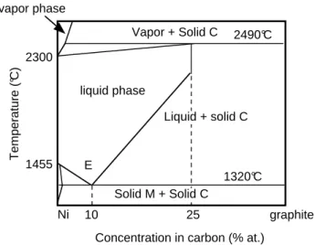
Concentration in carbon (% at.) E graphite vapor phase Vapor + Solid C 10 25 2490°C 1320°C 2300 1455 Liquid + solid C Solid M + Solid C
FIG. 6: Schematic phase diagram of the Ni-C system.
than the value deduced by Schwarz in its interpolation procedure: εp− εs = 8.0 eV,62 so that using our value
the 2s band is too high in energy. When interested in cohesive energies, this is not a problem since, as men-tioned previously, these s states do not contribute to the chemical bond.
We have now to determine the repulsive contribution to the total energy. As in the case of elemental metals, we assume a similar pairwise Born-Mayer (see Eq. (16)). The (A, p, q) parameters are fitted to the cohesive prop-erties of the hypothetical NaCl structure: equilibrium lattice parameter, bulk modulus and enthalpy of forma-tion ∆H of the carbide. The latter point is crucial here since we want to build a potential for Ni-C with good thermodynamic properties. The phase diagram shows clearly a tendency to phase separation, which indicates a positive enthalpy of formation (Fig. 6). The fact that the ordered phase Ni3C is metastable — it can be
pro-duced by mechanical alloying;72see also the observations
by Banhart et al.73 — indicates on the other hand that
it cannot be strongly positive. No reliable experimental value is available and we have therefore calculated ∆H from first principles calculations (ABINIT code). The enthalpy of formation per atom, ∆H, is defined as:
∆H = (EN aCl
N iC − EC− EN i)/2 , (18)
where EN aCl
N iC , EC and EN i represent the total
ener-gies of the rocksalt NiC compound (per formula), of the graphene sheet and of bulk fcc Ni (per atom), respec-tively. As expected, the enthalpy of formation of the carbide is found to be positive (∆H = 0.93 eV/atom). This is in good agreement with the values obtained from extrapolation of thermodynamic data.1,66 The
parame-ters used in our tight-binding model are A = 0.73 eV, p = 12.5 , and q = 3.2. The adjustments were performed in order to reproduce correctly the physical properties of the carbide, as shown in Table II. Finally the cut-off for the Ni-C interactions has been set at 3.20 ˚A.
TABLE II: Physical properties of NiC compound with the NaCl structure. Comparison of our tight-binding model with ab initio data.
Lattice ∆H (eV/atom) B (GPa) parameter (˚A)
ab initio 4.01 0.93 304
Present work 4.17 0.93 350
Let us summarize our discussion concerning the deriva-tion of a carbon-metal potential. The binding contribu-tion is mainly due to the pd hybridizacontribu-tion between the p states of carbon and the d states of the metallic el-ement. The values of the corresponding integrals have been obtained through an interpolation procedure, i. e. a tight-binding fit to the calculated first principles band structure of the equiatomic NaCl-like carbide. In the case of nickel, the relative position of the p and d atomic en-ergy levels has been chosen so that local charge neutrality is satisfied. The other parameters —repulsive term, de-pendence on distance of the attractive and repulsive parts — have been fixed through a fit to cohesive properties of the carbide, to its enthalpy of formation in particular.
At this point some comments are relevant. In the case of carbides (or nitrides), it is useful to distinguish be-tween cohesive energies and enthalpies of formation. The cohesive energy is in general defined as the total energy of the compound compared to atomic energies (energies of the constituents in their gaseous state). The enthalpy of formation compares the total energy to those of the con-stituents in their equilibrium crystalline states (graphene and fcc nickel in the case of NiC). Consider the exam-ple, detailed by Cottrell1, of TiC, which has the largest
cohesive energy in the 3d transition series, about 14.15 eV/formula. The cohesive energy of Ti and C are equal to 4.85 eV/at and to 7.4 eV/at respectively, so that the enthalpy of formation per formula (or per carbon atom) is equal to -1.90 eV. The enthalpy of formation is a small percentage of the cohesive energy of the constituents. In other terms, all bonds, metal-metal, carbon-carbon, and carbon-metal bonds are strong and the stability of the carbides is a relatively delicate balance between them. Starting from pure Ti in the fcc phase (which has a cohe-sive energy very close to that of the stable hcp phase) the introduction of carbon atoms in the octahedral intersti-tial sites distorts slightly the host lattice, hence some loss of d bonding energy, but the main balance is between the energy gain due to the first neighbour pd hybridization and the energy loss due to the breaking of C–C bonds. A quite similar argument applies also to NiC whose en-thalpy of formation per formula, about +1.8 eV should be compared to the cohesive energies of nickel and carbon, 4.5 eV and 7.4 eV, respectively. Even if the compound NiC does not exist, the Ni-C bond is very strong and local ordered configurations can be metastable. This property is probably at the root of the interesting catalytic prop-erties of Fe, Co, and Ni.
VI. VALIDATION OF THE MODEL The difficulty in the derivation of a complete potential for carbides was clearly the nickel-carbon part. Once all parameters have been fitted, the model can be applied to any atomic configuration of carbon and nickel atoms, provided that the parameters do not depend too much on the concentration of carbon atoms. In order to test this assumption and to test the transferability of our poten-tial, we have studied many different situations. In Sec. VI A the solubility of carbon in nickel is considered, in the bulk as well as at, or close to, the surface. Interac-tions of Ni atoms with a graphene sheet are discussed in Sec. VI B. The clock reconstruction observed when car-bon and other light elements are deposited on a (100) Ni surface is then analyzed in Sec. VI C. Sec. VI D presents a discussion of the (epitaxial) formation of graphene on Ni or Co (111) surfaces. Finally recent applications of our energetic model to the study of the catalytic growth of carbon nanotubes are summarized in Sec. VI E.
A. Carbon solubility in nickel
A quantity of great interest is the heat of solution, ∆Hsol, of a C interstitial atom in crystalline Ni.
Experi-mental and ab initio data exist for the Ni-C solid solution in the paramagnetic state,74 which allows us to make a
critical assessment of our tight-binding model. The heat of solution of C in Ni with respect to graphene is calcu-lated according to the formula:
∆Hsol= EN i+C− (EN i+ EC), (19)
where EN i+C is the total energy of the interstitial Ni+C
system, EN i is the energy of the Ni system without C,
and ECis the energy per C atom in graphene. In the fcc
Ni lattice, two high-symmetry interstitial sites are avail-able for C occupation: the octahedral and the tetrahedral site. The most likely location for C in the fcc lattice is believed to be at octahedral interstitial sites, which is confirmed by first principles calculations.74,75
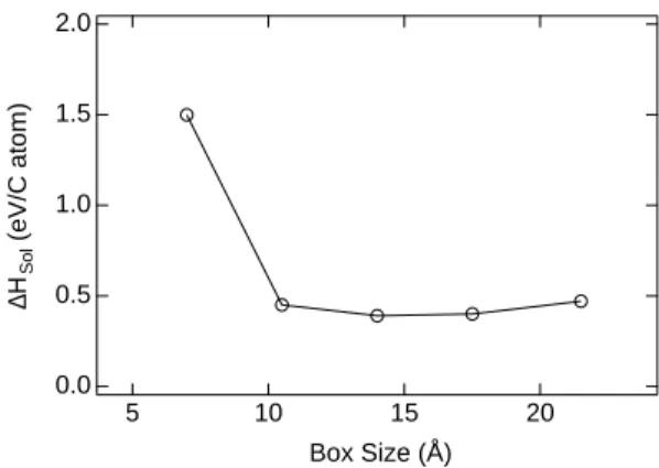
In the present work, only this configuration has been investigated, the bulk fcc Ni being simulated by a finite box of dimensions up to 6 × 6 × 6 in units of fcc unit cells, with periodic boundary conditions along the three axis. This was necessary to obtain converged results (see Fig. 7). Actually the octahedral site of fcc Ni is a little bit too small to accomodate a carbon atom which therefore pushes its first neighbour Ni atoms. This induces long range elastic interactions between the images of the car-bon atom due to the periodic boundary conditions. Using a simulated annealing procedure, we find that the six Ni atoms, surrounding the interstitial C atom are displaced of about 0.15 ˚A in such a way that the Ni-C bonds have a length about 1.90 ˚A which is close to the equilibrium dis-tance in the rocksalt structure, equal to 2 ˚A. Finally we obtain a heat of solution within our tight-binding frame-work equal to 0.45 eV, in good agreement with the 0.43
2.0 1.5 1.0 0.5 0.0 ∆H Sol (eV/C atom) 20 15 10 5 Box Size (Å)
FIG. 7: Variation of the calculated energy of dissolution as a function of the size of the supercell.
eV value found experimentally and higher than the 0.2 eV found in previous DFT works.74This better agreement of
the tight-binding semi-empirical scheme is certainly for-tuitous, but the “first principles” calculations have also some weaknesses. First the result depend significantly on the approximation used: GGA versus LDA, form of the exchange-correlation functional, nature of the pseudopo-tential, etc. Another problem is related to the size of the supercell used. In units of the fcc unit cell the latter authors used a 2 × 2 × 2 box which is probably too small according to our calculations. Other possible reasons for the theoretical underestimate of ∆Hsol are discussed in
detail by Siegel and Hamilton.74 Recent calculations by
Zhu et al. with box sizes up to 3 × 3 × 3 show similar results .75In any case the positive sign of ∆H
solis
consis-tent with the positive value of the enthalpy of formation discussed in Sec. V. Both quantities should indeed be comparable since carbon atoms in the NaCl structure do not interact directly. The difference comes again from the induced elastic interactions.
It is useful at this point to recall that one has to be very careful with the cut-offs of the potential (hopping integrals in particular) when performing such structural relaxations. These cut-offs are generally chosen to lie in between coordination shells of the crystalline structure of reference, but the coodination numbers can change dur-ing the relaxation process, which can induce unphysical discontinuities. Although well-known this type of arti-fact is not always easily detected. In our case we a have a nice tool because of the possibility to calculate local energies on different atoms. Although these energies de-pend on the local environments it is fairly easy to detect unphysical variations, and to modify the cut-offs. The values given in this article have been chosen so as to avoid problems in all cases which have been investigated. Another test of the model is to study how the heat of solution is modified in the presence of a surface. We have calculated this energy for different positions of the carbon atom on a (111) surface or just below it. The most favourable position is the subsurface position, in between the first (111) planes, so that the carbon atom
has a full octahedron environment.76 The adsorption or
adhesion energy is found equal to -8.25 eV, which is in good agreement with first principles calculations.15This
quantity, frequently used when considering catalysis pro-cesses, refers to the energy of atomic carbon. To convert it into an heat of solution, we have to substract the forma-tion energy of graphene, equal to -7.42 eV. The enthalpy of solution is therefore equal to -0.83 eV, which means that the solution process is exothermic close to the sur-face, whereas it is endothermic in the bulk. Although this effect is perhaps overemphasized within our model, its physical origin is clear. The positive sign of ∆Hsol
in the bulk is principally due to a size effect, the sur-rounding nickel atoms being pushed by the carbon atom, but this is counterbalanced by the elastic response of the crystal. In the presence of a surface the relaxation pro-cess is easier and the elastic energy cost is lower. This clearly shows that this size effect favours the segregation of carbon towards surfaces. More details are given in Ref. [15]. Some results obtained for the (100) surface16
are discussed below.
B. Interaction of Ni atoms with a graphene sheet
We have studied the interaction of Ni atoms with a graphene sheet. Two possible stable positions are gen-erally considered where the Ni atom is either above a carbon atom (top position) or above the centre of an hexagonal carbon ring (hole position). For the late 3d transition elements, the hole position is preferred.18,77
We have checked that within our model. Using a simu-lated annealing Monte Carlo procedure, the final position of a Ni atom is always the hole position, whatever the ini-tial condition. The binding energy is found equal to 3.5 eV, which is in semi-quantitative agreement with the 2.5 eV value obtained by Duffy and Blackman in a cluster (DMOL) calculation.77 The agreement is also good for
the values of the height of the adatom above the sheet: 1.57 ˚A in our calculation instead of 1.53 ˚A in Ref. [77].
We have also calculated the energy of substitution of a C atom in a graphene sheet by a Ni atom. The ground state structure obtained again after a simulated anneal-ing procedure is shown in Fig. 8. The Ni atom is found displaced out of the graphene sheet by 1.1 ˚A, which is close to the 1.0 ˚A value given by Banhart et al. on the basis of electronic microscopy observations as well as of first principles calculations.73The energy of substitution
is found equal to 10.8 eV, to be compared to the 9.5 eV ab initiovalue. This strong positive value shows that this substitutional defect can hardly be stable. Banhart et al. argued that Ni atoms most probably fill existing vacan-cies created by the electron beam in their transmission electron microscopy observations.
FIG. 8: Final position, after relaxation, of a substitutional Ni atom in a graphene sheet; top and side views.
C. Clock reconstruction on Ni (100) surfaces The interaction of carbon with transition-metal sur-faces has been widely studied. Carbon chemisorption on Ni surfaces in particular has been considered in detail, from an experimental point of view, in a series of papers by Blakely and co-workers,78as well as from a theoretical
point of view.2,79 In the case of the (100) surface, which
has a simple square lattice structure, carbon at low cov-erage occupies the hollow semi-octahedral sites, with an adsorption energy equal to -8.21 eV within our model,16
in good agreement with experimental and ab initio data. Here again the latter ones depend significantly on the ap-proximation used.80 At higher coverage, carbon, as well
as many other elements (N, O, S), form a c(2 × 2) su-perstructure. This occcurs for a surface coverage beyond one third of a monolayer in the case of carbon. Contrary to sulfur and oxygen, carbon and nitrogen atoms induce a reconstruction of the outermost layer of nickel atoms of p4g symmetry called a “clock” reconstruction where the top-most Ni atoms move around C atoms by alternate clockwise and counterclockwise rotations (see Fig. 9 bot-tom). The distortion preserves the shape of the carbon squares, while the nickel atoms, which are not surround-ing the C atoms, become rhombi. This reconstruction is clearly induced by the stresses exerted by the carbon atoms on their surrounding nickel atoms (see below). A lot of experimental and theoretical studies have been de-voted to this reconstruction.81,82,83,84
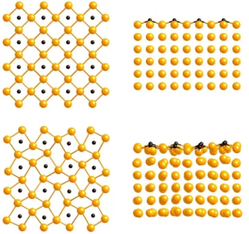
To test our model, we have performed simulated
FIG. 9: Clock reconstruction obtained within our tight-binding model. Top: top and side view of the initial sim-ulation box. Bottom: same views after clock reconstruction.
nealing simulations on a slab of nickel (208 atoms) with(100) surfaces and covered by C atoms. A 20 ˚A thick vacuum region was introduced along the z axis and peri-odic boundary conditions were applied in the two other directions. The slab size is 12.47 × 12.47 × 8.79 ˚A3. 16
carbon atoms are deposited above the surface made of 32 Ni atoms in a c(2×2) geometry, corresponding to a cover-age equal to 0.5 ML (see Fig. 9 top). In the present case, all the atoms in the system are fully relaxed. During the simulation, we observe that the C atoms move slightly outwards, at about 0.35 ˚A above the fourfold hollow site, whereas the Ni atoms of the first layer of Ni atoms self-organize to adopt the p4g symmetry (see Fig. 9 bottom). Our results, summarized in Table III, are in very good agreement with previous first-principles calculations and experimental data.
In order to understand the driving force for the p4g symmetry reconstruction on fcc (100) surfaces, Klink et al. performed a systematic experimental study of the changes in surface stress as a function of coverage of car-bon using STM.81The results can be briefly summarized
as follows. In the low coverage phase, θ < 0.2 ML, the C atoms adsorb in fourfold hollow sites. Then, the four Ni atoms surrounding each carbon atom are displaced ra-dially to allow the C atoms to remain embedded within the Ni surface so that they are fivefold coordinated (one Ni atom below and four in-plane atoms. Beyond θ = 0.2 ML, the surrounding Ni atoms can no longer be pushed away radially. Then, the collective p4g clock reconstruc-tion in which the squares of Ni atoms surrounding the C atoms rotate insures that these C atoms keep their semi-octahedral environment, the stress being transfered on
Energy (eV/at) 0.8 0.6 0.4 0.2 0.0 Displacement (Å)
δ
FIG. 10: Total energies as a function of the displacement δ for different values of distance carbon atoms and the surface plane.
the empty Ni squares which transform into rhombi. To study this process in more detail, we have performed to-tal energy calculations for different values of δ, the ampli-tude of the in-plane displacement of the first-layer metal atoms upon reconstruction. The initial system consid-ered here is the same as that described previously. Our results presented in Fig. 10 for different adatom-surface distances show clearly two regimes. For distances lower than 0.4 ˚A, the most stable configuration is the recon-structed one, the amplitude of which decreases when the adatom moves upwards. Above 0.4 ˚A, the reconstruc-tion is no longer stable. Thus, big atoms which cannot approach the surface do not provoke the clock reconstruc-tion. For instance, a half monolayer coverage of Cl, S, and O on Ni(100) results in structures with small or no recon-struction. The comparison of the behaviours of oxygen on a Rh (100) and a Ni (100) surface is very interesting from this point of view: rhodium (3.80 ˚A) has a lattice parameter larger than nickel (3.52 ˚A) and offers more room for an oxygen atom, and actually the reconstruc-tion is observed in Rh and not in Ni.87
D. Graphene on Ni (111)
Much less observations are available concerning recon-structions of the Ni (111) surface, apart from STM stud-ies by Klink et al.88 indicating a possible clock
recon-struction similar to the one described previously. This would imply a removal of Ni atoms, which, to our
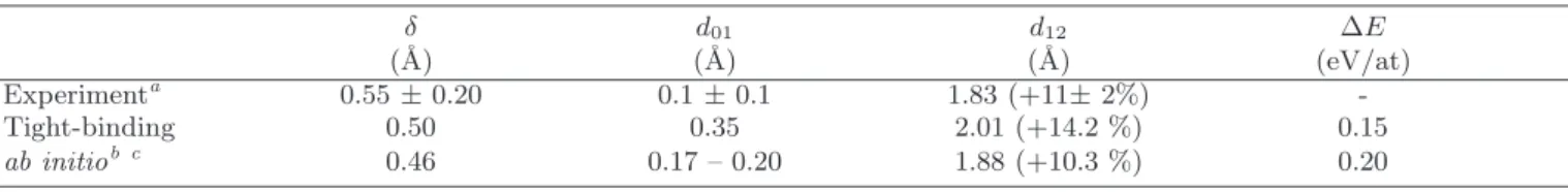
TABLE III: Energetic and structural characteristics of the clock reconstruction obtained within our tight-binding model com-pared to experimental and ab initio data. δ: amplitude of the in-plane displacement of the first-layer metal atoms characterizing the clock reconstruction; d01 : C-surface distance; d12: distance between the first and the second Ni plane. The percentage
between parenthesis indicate the amplitude of the expansion with respect to pure Ni. ∆E is the energy difference between the symmetric c(2 × 2) structure and the reconstructed one.
δ d01 d12 ∆E (˚A) (˚A) (˚A) (eV/at) Experimenta 0.55 ± 0.20 0.1 ± 0.1 1.83 (+11± 2%) -Tight-binding 0.50 0.35 2.01 (+14.2 %) 0.15 ab initiob c 0.46 0.17 – 0.20 1.88 (+10.3 %) 0.20 aFrom Ref. 85. bFrom Ref. 83. cFrom Ref. 86.
edge, has not been confirmed experimentally or theoreti-cally. On the other hand the formation of graphene sheets on Ni (111) has been the subject of countless studies, principally because of the interest of such surfaces, in catalysis processes.2,89 The recent revival of interest for
graphene has also prompted many studies,90 one
chal-lenge being to be able to grow in a controlled manner graphene sheets on different substrates. Apart from the original exfoliation method, epitaxial sheets have been shown to grow via the evaporation of SiC surfaces.91,92
But it has been soon rediscovered that Ni or Co (111) surfaces offer almost perfect templates for the growth of epitaxial graphene sheets. Actually, the in-plane lattice constants of graphene match the surface lattice constants of (111) Co and Ni almost perfectly, with for example a lattice mismatch of only 1.3% for Ni. Other substrates, Cu, Ir, Pd, Pt, Re, Ru, . . . have also been studied.93
Different epitaxial positions are possible, but there are still controversies — experimental as well as theoretical — concerning their relative stabilities, the values of the energies of interaction and the interplane equilibrium dis-tance. Values ranging from 2 to 3 ˚A for the latter one are for example reported in the literature.15,94,95,96This
is perhaps no so surprising: experimentally many factors, impurities, steps, can play a role. Theoretically it is also known that the (Van der Waals) long range interactions involving graphene sheets within graphite are difficult to handle within standard DFT codes. The dispersion in the calculated adhesion energies is smaller. This energy is generally found to be slightly (negative) attractive, in the range -0.05 — -0.1 eV per carbon atom.15
Using our model, we have considered a graphene layer in perfect epitaxy on a Ni slab in the so-called fcc ge-ometry, where half of the carbon atoms are above the Ni atoms whereas the other half occupies the so-called fcc positions. We have then relaxed the atomic positions us-ing a Monte Carlo simulated annealus-ing procedure. The result is an adhesion energy equal to -0.03 eV and an equilibrium interplane distance equal to 2.19 ˚A in very good agreement with ab initio calculations. Here again our potential behaves as it should. Single carbon atoms interact strongly with Ni (strong adhesion energy), but
once the sp2 covalent bonds have been established, the
resulting graphene sheet no longer interacts with the Ni surface. This behaviour, also consistent with the ten-dency of the Ni-C to phase separation, would of course be difficult to reproduce using phenomenological potentials. Notice also that the weakness of the adhesion energy of graphene shows that, as far as energetic properties are concerned, the presence of available π orbitals of carbon do not play a significant role: the possible energy gain due to pd C–Ni bonds is counterbalanced by a loss of direct π − π bonding, the latter one being maximum for a band filling corresponding to pure graphene. The hy-bridization of the π states with the d3z2−r2 Ni states on the other hand does exist18,79,97,98 and has been clearly
observed close to the Fermi level.99,100
A stronger test of our potential is to start from a con-figuration such as a solid solution of carbon in nickel and to see whether it can predict carbon segregation towards the surface. We have developed a full thermodynamic model using Monte Carlo simulations within the grand-canonical ensemble, where the control parameter is the carbon chemical potential. This is described in detail elsewhere15 and we just recall some results here. When
the chemical potential increases, more and more carbon atoms are added in the system, and basically, as shown in Fig. 11, four types of configurations corresponding to different reaction steps are identified: single C atoms ad-sorbed on the surface or incorporated in interstitial sites, chains creeping on the surface, detached sp2 C layers,
and finally a three-dimensional amorphous C phase.
E. Application: nucleation of nanotube embryos Since an important motivation to derive an energetic model for metal-carbon systems was to understand the role of catalysts in the growth of carbon nanotubes, let us finally summarize the results which we have already been obtained in this field.
Starting from a small nickel cluster instead of the (111) surface treated above, we have undertaken studies of the nucleation of carbon caps. Here again, there is an optimal
FIG. 11: Equilibrium structures (side and top views), at 1000 K, obtained from Monte Carlo simulations performed on a (111) Ni slab for increasing values of the chemical potential µC: -6.00, -5.75, -5.25, and -4.50 eV/atom. In (a) carbon atoms occupy
interstitial, octahedral, sites; in (b) they form linear chains on the surface; then in (c) a graphene layer appears and finally, in (d) a thick amorphous phase begins to grow.
FIG. 12: Successive stages of the nucleation of a C cap on a 55 atom cluster of nickel for a chemical potential equal to 5.25 eV/atom.
chemical potential window to nucleate these graphitic caps whose curvature match the local curvature of the catalyst particle (see Fig. 12). The chemical potential has to be large enough to insure a sufficient concentra-tion of carbon atoms at the surface. It should also be small enough to avoid the formation of a thick amor-phous layer. The role of the catalyst is to confine carbon atoms on or close to the surface. This shows the impor-tance to have strong interactions between the metallic elements and isolated carbon atoms, and explains why the late transition elements are good catalysts. They do interact strongly with carbon atoms, but weakly with graphitic structures. These arguments agree with other studies based on ab initio calculations12,101 and are
de-tailed elsewhere.10
The case treated above corresponds to a situation fre-quently encountered in chemical vapour deposition pro-cesses where the nanotubes grow in a tangential mode, the diameter of the tubes being related to the size of the
catalyst particle. In other cases, particularly in the high temperature synthesis, the nanotubes grow perpendicu-larly to the surface.5 Arguments based on classical
nu-cleation and growth thermodynamic models have been put forward to understand how this can happen.102,103
Carbon atoms at the surface of the metallic catalyst are assumed to condense in the form of graphene flakes. The metallic substrate can then help to saturate the dangling bonds and this favours the formation of a cap, the en-ergy cost due to the curvature induced by the presence of pentagons being more than compensated by the reduc-tion of the number of dangling bonds.103This model has
been partly confirmed by Fan et al.104 who performed
ab initioenergy calculations of different arrangements of carbon atoms on a Ni(100) surface, but these calculations are computationally very demanding and the structures cannot be fully relaxed.
We have therefore used our model which permits such atomic relaxations. Examples are shown in Fig. 13. The possibility to analyze local energy distributions has also allowed us to determine which atoms (carbon or nickel), and to what extent, are stabilized when various carbon clusters are put in contact with a metallic surface. Fi-nally the adhesion process of carbon sheets on Ni (100) is slightly more complex than anticipated. The adhesion energy of flat sheets is mainly due to the energy gain of the nickel atoms below these sheets. When they curve to form caps, the energy gain becomes concentrated on the carbon and nickel atoms close to their edge. In this case one might argue that dangling bonds are saturated, but finally, this is a weak effect which does not play very much in favour of curved caps: the energy of adhesion of flat and curved sheets are similar and small compared to
FIG. 13: Equilibrium configurations of carbon clusters on a (100) Ni surface: (a) planar polyaromatic cluster; (b) nan-otube embryo. Notice the fairly large displacements of Ni atoms below the clusters.
dangling bond energies, for small clusters at least. This is fully discussed in Ref. [16].
VII. CONCLUSION
In this work we have presented a model based on the tight-binding approximation which provides an efficient tool to calculate the bonding energies in the Ni-C sys-tem, total energies being obtained by adding empirical repulsive terms. The model is both simple and accurate. We have taken advantage of the fact that the band en-ergies are not very sensitive to details of the electronic structure to use a moment-recursion technique at the level of a fourth moment aproximation. The use of s, p, d atomic orbitals and of the corresponding transfer inte-grals insures on the other hand that the different types of metallic and covalent chemical bonds are correctly de-scribed.
C-C interactions are defined from a slight modification of the model introduced by Xu et al..34 Due to the use
of a complete (s, p) basis for the carbon states, all types of covalent spn bonds can be modelized. The model is
shown to reproduce several properties such as the dia-mond to rhombohedral-graphite transition or the energy of local defects such as the Stones-Wales defect. Ni-Ni interactions are obtained using a fairly standard tight-binding approximation including d states only. We have shown however that one has to be careful to choose band fillings of the d band such that the fcc structure is sta-ble and that the elastic shear moduli are positive. The
crucial point in this work is the derivation of Ni-C in-teractions. They have been constructed from a detailed study of the electronic structure and bonding properties of transition metal carbides.
The final full model can be applied to any atomic figuration of carbon and nickel atoms, and we have con-sidered many different situations involving a large variety of Ni-C interactions to test the model: heat of solution in the bulk, at the surface or close to it. Adatoms: nickel on carbon, carbon on nickel. The case of the spectacular clock reconstruction ot the Ni (100) surface induced by carbon atoms has been studied in detail as well as the epitaxy between graphene and Ni (or Co) surfaces. In all cases the model is fairly accurate when compared to experiment or to ab initio calculations: our model has a high degree of transferability. Actually typical error bars are of the order of 0.1–1eV compared to total energies of the order of 5–10 eV. This is obviously not negligible but it should be kept in mind that ab initio methods are frequently not better from this point of view. They show dispersions of the same order of magnitude, principally in the case of point or localized defects where atomic re-laxations can be so important that it is difficult to obtain converged results. On the other hand most phenomeno-logical models can hardly be transferable and are not very reliable when severable types of Ni-carbon bonds compete.
A further advantage of our model is that it can be fairly easily generalized to other metal-carbon systems, since we know semi-quantitatively how the different pa-rameters — transfer integrals, atomic energy levels, etc. — vary with the nature of the metallic element. A more difficult point is related to charge transfer. In the case of Ni we have argued that we can avoid treating it explic-itly by adjusting the position of the atomic energy levels. This can no longer be done in the case for example of the Ti-C system where charge transfers towards carbon can be of the order of one electron. In this case a Hartree-like treatment should at least be used where the atomic energy levels depend on the atomic environment. From a practical point of view, it will be possible to define inter-polation procedures similar to the one used in this work to vary the effective number of d electrons. Another chal-lenge is to include magnetism since magnetic and struc-tural effects can be strongly coupled as in the case of Fe105 and of Fe-C.106 This is currently under progress.
More complex tight-binding models can be used as well to handle these problems,18,36,107 but the price to pay is
generally fairly high in terms of parameters to be fitted and of computational cost.
Acknowledgments
Fruitful discussions with K. Albe, J.-Ch. Charlier, G. Hug, and Ph. Lambin are gratefully acknowledged.

![TABLE I: Comparison of our tight-binding d model with experimental data. The experimental values for fcc Ni and hcp Co are taken from Ref.[49]; those for fcc Co from Ref.[50] and the surface energies from Ref.[51].](https://thumb-eu.123doks.com/thumbv2/123doknet/12726008.357028/7.892.82.843.127.303/table-comparison-binding-experimental-experimental-values-surface-energies.webp)