Geospatial data for developing nutrient SPARROW models for the Midcontinental region of Canada and the United States

(1)

Publisher’s version / Version de l'éditeur:

Technical Report (National Research Council of Canada. Ocean, Coastal and

River Engineering); no. OCRE-TR-2018-014, 2018-12-21

NRC Publications Archive Record / Notice des Archives des publications du CNRC :

https://nrc-publications.canada.ca/eng/view/object/?id=0e5ed829-58a1-4742-a198-8322dbdc327c

https://publications-cnrc.canada.ca/fra/voir/objet/?id=0e5ed829-58a1-4742-a198-8322dbdc327c

NRC Publications Archive

Archives des publications du CNRC

For the publisher’s version, please access the DOI link below./ Pour consulter la version de l’éditeur, utilisez le lien DOI ci-dessous.

https://doi.org/10.4224/23004810

Access and use of this website and the material on it are subject to the Terms and Conditions set forth at

Geospatial data for developing nutrient SPARROW models for the

Midcontinental region of Canada and the United States

Vouk, Ivana; Burcher, Richard S.; Johnston, Craig M.; Jenkinson, R. Wayne;

Saad, David A.; Gaiot, John S.; Benoy, Glenn A.; Robertson, Dale M.; Laitta,

Michael

(2)

Geospatial Data for

Developing Nutrient

SPARROW Models for the

Midcontinental Region of

Canada and the United States

Report No.: OCRE-TR-2018-014

Date: December 21, 2018

Authors: Ivana Vouk

1

_{, Richard S. Burcher}

1

_{, Craig M.}

Johnston

2

_{, R. Wayne Jenkinson}

3

_{, David A. Saad}

2

_{, John}

S. Gaiot

4

_{, Glenn A. Benoy}

3

_{, Dale M. Robertson}

2

_{, and}

Michael Laitta

3 1 National Research Council of Canada – Ocean, Coastal, River Engineering Research Centre 2 U. S. Geological Survey 3 International Joint Commission 4 Ontario Ministry of Natural Resources and Forestry

(3)

(4)

EXECUTIVE SUMMARY

Through the International Watersheds Initiative of the International Joint Commission (IJC), the Spatially-Referenced Regressions on Watershed attributes (SPARROW) model developed by the U.S. Geological Survey (USGS) is being applied to the Great Lakes, Rainy River – Lake of the Woods and Red-Assiniboine basins. The objective of this binational application of the SPARROW model is to better understand and quantify the sources of phosphorus (P) and nitrogen (N) that contribute to regional water-quality issues like algal blooms and eutrophication in Lake Erie and other parts of the Great Lakes, as well as Lake of the Woods. Led by the IJC, a team of researchers from the National Research Council of Canada – Ocean, Coastal and River Engineering Research Centre, USGS, and IJC are extending the SPARROW modelling work previously completed for the Red-Assiniboine basin and the U.S. portions of the Great Lakes, Ohio, Upper Mississippi, and Souris-Rainy river basins to cover all of the Great Lakes, Rainy River – Lake of the Woods and Red-Assiniboine basins. The current effort is termed the Midcontinent SPARROW modelling study.

This report describes the data used to develop the Midcontinent SPARROW models, specifically the sources of original data, assembling the data, and the processing and harmonization required between the U.S. and Canada data needed to produce these models. Details provided include the:

·

development of a digital stream network and related catchments – most significantly in the Canadian regions of the Great Lakes and Rainy River – Lake of the Woods basins where these data were not available to create a seamless binational network across the model domain;

·

calculation of variables to aid in the determination of in-stream and in-reservoir decay of P and N;

·

quantification of Canadian diversions within the Midcontinental region (i.e., Lake St. Joseph, Long Lake and the Ogoki Reservoir);

·

development of binational input nutrient sources considered for model development (i.e., land cover, inorganic farm fertilizer, manure, atmospheric deposition, point-source pollution from wastewater-treatment plants and contribution from non-modelled watersheds); and

·

development of delivery variables considered to be most predominant (i.e., temperature, precipitation and ensuing runoff, soil permeability and clay content, slope of the catchments, and tile drainage).

The majority of the geospatial data collection and processing was required for Canadian datasets because many of the U.S. datasets were already assembled for previous SPARROW model applications in the U.S. The task of harmonizing data between the U.S. and Canada was important to ensure consistency of the datasets used in the models. The harmonized digital stream network, delineated catchments and input data for each catchment (i.e., source and delivery variables), created for the Midcontinent SPARROW models, are available for download at url:https://doi.org/10.4224/300.0001.

(5)

Figures

Figure 1: States and provinces comprising the Midcontinental region. ... 2

Figure 2: The Midcontinent SPARROW models domain. The inset identifies the locations of Brokenhead, Whitemouth and Whiteshell Rivers basins... 4

Figure 3: Final Midcontinent SPARROW model digital stream network – colour coded to indicate the original data source(s). ... 9

Figure 4: Calibration points (monitoring stations) used to preserve stream segments during thresholding and generalization... 10

Figure 5: Midcontinent SPARROW model catchments. Enlarged view of the catchments is provided in the inset as an example, indicated by the yellow rectangle the red arrow is pointing to on the larger map. ... 13

Figure 6: Validation results for estimated versus observed flows (left) and drainage areas (right) in the Great Lakes basin. The 1:1 reference line is indicated with a red line. ... 15

Figure 7: Validation results for estimated versus observed flows (left) and drainage areas (right) in the Winnipeg River basin. The 1:1 reference line is indicated with a red line. ... 15

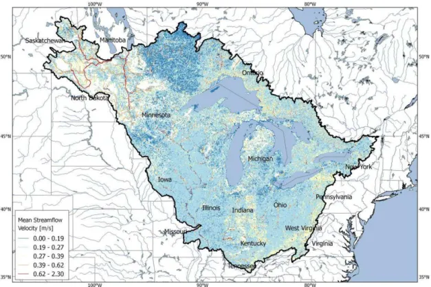
Figure 8: Estimated velocity in streams throughout the Midcontinental region. ... 16

Figure 9: Estimated inverse of hydraulic load throughout the Midcontinental region. ... 17

Figure 10: Stream diversions in Canada (with respect to the extents of the Midcontinental region). The inset provides a close-up view of Lake St. Joseph, Ogoki Reservoir and Long Lake, with red arrows indicating the direction of flow diversion. Lake Nipigon is identified in the inset. ... 18

Figure 11: Harmonized land cover throughout the Midcontinental region. ... 20

Figure 12: Total phosphorus (above) and total nitrogen (below) input rates, by catchment, throughout the Midcontinental region. ... 22

Figure 13: Total phosphorus (above) and total nitrogen (below) input rates, by catchment, from manure spread on agricultural and pasture lands throughout the Midcontinental region. ... 24

Figure 14: Atmospheric deposition rates of total nitrogen from CMAQ, by catchment, throughout the Midcontinental region. ... 25

Figure 15: Wastewater-treatment plants used in the Midcontinent SPARROW models. ... 27

Figure 16: Mean annual air temperature, by catchment, throughout the Midcontinental region. ... 28

Figure 17: Mean annual precipitation by catchment, throughout the Midcontinental region. ... 29

Figure 18: Mean annual runoff by catchment, throughout the Midcontinental region. ... 30

Figure 19: Soil permeability (above) and clay content (below) by catchment, throughout the Midcontinental region. ... 32

Figure 20: Mean catchment slopes by catchment, throughout the Midcontinental region. ... 33

Figure 21: Percentage of the catchment underlain with tile drains, by catchment, throughout the Midcontinental region. ... 35

(8)

Glossary

high-resolution NHD 1:24,000-scale national hydrographic dataset

HYDAT Environment and Climate Change Canada HYdrological DATabase that contains computed data from Water Survey of Canada’s hydrometric gauges

medium-resolution NHDPlus 1:100,000-scale national hydrographic dataset

SPARROW SPAtially Referenced Regression On Watershed attributes model is a spatially-referenced regression-based model

developed by the U.S. Geological Survey that relates patterns in loads of water-quality parameters to human activities, climate, hydrology, geology and physiography

(9)

Acronyms

3DEP 3D Elevation Program (U.S.)

AAFC Agriculture and Agri-Food Canada

CaPA Canadian Precipitation Analysis

CCS Census consolidated subdivisions (Canada)

CD Census divisions (Canada)

CDED Canadian Digital Elevation Dataset

CFS Canadian Forest Service

CMAQ Community Multiscale Air Quality Modeling System (U.S.)

DEM Digital elevation model

ECCC Environment and Climate Change Canada

EWC Enhanced Watercourse (Ontario)

GIS Geographic information system

GL Great Lakes

HUC12 12-digit Hydrologic Unit Code (U.S.)

IWI International Watersheds Initiative (IJC)

MCWS Manitoba Conservation and Water Stewardship

MOECC Ministry of Ontario Environment and Climate Change

MSD Manitoba Sustainable Development

NAWQA National Water-Quality Assessment (U.S.)

NED National Elevation Dataset (U.S.)

(10)

NTDB National Topographic Database (Canada)

OIHD Ontario Integrated Hydrology Data

OHN Ontario Hydro Network

OMAFRA Ontario Ministry of Agriculture, Food and Rural Affairs

OMNRF Ontario Ministry of Natural Resources and Forestry

PRISM Parameter-elevation Regressions on Independent Slopes Model

RA Red-Assiniboine River

SAS Statistical Analysis Software

SPARROW SPAtially Referenced Regressions On Watershed attributes

SSDA Sub-sub-drainage area

STATSGO STATe Soil GeOgraphic database (U.S.)

TN Total Nitrogen

TP Total Phosphorus

USEPA U.S. Environmental Protection Agency

USGS U.S. Geologic Survey

WBD Watershed Boundary Dataset

WR Winnipeg River

WSC Water Survey of Canada

(11)

This report is dedicated to the memory of Craig Johnston (1969–2018). A GIS specialist with the U.S.

Geological Survey, Craig was an invaluable member of the binational SPARROW modelling team who helped introduce the International Joint Commission to the SPARROW approach. He was our leading light on the development of binational stream networks – the true backbones of the models. Craig had a wonderful spirit and is dearly missed.

(12)

Acknowledgements

The authors are grateful to the National Research Council’s staff: Vahid Pilechi, Sean Ferguson and student Isabelle Cheff for their efforts in processing much of the Canadian source and delivery variables, and to Anne Collins for processing the initial Great Lakes stream network. The authors would like to thank Glenn Lelyk of Agriculture and Agri-Food Canada (who had devoted a number of hours to provide a product relevant to the effort) for processing and providing Canadian soils information. The authors would also like to thank Jason Vanrobaeys of Agriculture and Agri-Food Canada and Mark Henry of Statistics Canada for guidance on Canadian agricultural outputs. Finally, the authors would like to acknowledge other researchers, scientists and water resource managers who answered our phone calls and replied to our emails: Elaine Page, Geoff Reimer and Tara Wiess (Manitoba Sustainable Development), Andy Kester (Ontario Ministry of Agriculture, Food and Rural Affairs), Doug Johnson (Saskatchewan Water Security Agency), Antonette Arvai (International Joint Commission), Bruce Davison (Environment and Climate Change Canada), Pam Minifie (Saskatchewan Ministry of Environment) and Amanda Giamberardino (Fertilizer Canada). Any use of trade, firm, or product names is for descriptive purposes only and does not imply endorsement by the Canadian and U.S. Governments.

(13)

1 Introduction

Many watersheds straddle the border between Canada and the United States (U.S.). Through the International Watersheds Initiative (IWI) of the International Joint Commission (IJC)1_{, the Spatially Referenced Regressions}

on Watershed attributes (SPARROW) model, developed by the U.S. Geological Survey (USGS), is being applied to the Midcontinental region of North America (Figure 1). This region consists of the Great Lakes (GL) basin, Winnipeg River (WR) basin, Red-Assiniboine River (RA) basin, Upper Mississippi River basin and Ohio River basin, including the basins between the WR and RA (i.e., Brokenhead River, Whiteshell River and Whitemouth River basins that for the purpose of this study are considered part of the WR basin) (Figure 2). This large area spans parts of Saskatchewan, Manitoba, and Ontario in Canada, and the upper midwest and Great Lakes states of the U.S., as illustrated in Figure 1. The motivation for the study is to better understand and quantify the sources of phosphorus and nitrogen that contribute to regional water-quality issues like algal blooms and eutrophication in Lake Erie and other parts of the Great Lakes, as well as Lake of the Woods basins.

Led by the IJC, an international team was assembled for the project, including researchers from the National Research Council of Canada – Ocean, Coastal and River Engineering (NRC-OCRE) Research Centre, USGS and the Ontario Ministry of Natural Resources and Forestry (OMNRF). Successful development of the

geospatial dataset required significant contribution from the following additional Canadian federal and provincial collaborators: Environment and Climate Change Canada (ECCC), Agriculture & Agri-Food Canada (AAFC), Manitoba Sustainable Development (MSD) formerly known as the Manitoba Conservation and Water

Stewardship (MCWS), and Ministry of Ontario Environment and Climate Change (MOECC). This model builds on the experience gained from the USGS application of the SPARROW model for the National Water-Quality Assessment (NAWQA) Project studying the U.S. portions of the Great Lakes, Ohio, Upper Mississippi, and Souris-Red-Rainy river basins (Robertson and Saad, 2011) and the SPARROW modelling work previously completed on the RA basin (i.e., RA SPARROW models) (Benoy et al., 2016). It also takes advantage of the IWI Data Harmonization Project, which pioneered the development of interoperable hydrographic and geospatial datasets for transboundary basins along the international border (Laitta, 2010).

(14)

Figure 1: States and provinces comprising the Midcontinental region.

Lake Superior

Lake Ont ario Lake Huron

Lake Winnipeg

Lake Nipigon Qu’Appelle River

(15)

2 Background

2.1 The SPARROW model

SPARROW is an empirically based spatially-referenced regression modelling approach developed by the USGS that relates patterns in loads of water-quality parameters to human activities, climate, hydrology, geology and physiography (Schwarz et al., 2006). The SPARROW model has been applied in many regions including the entire continental U.S., as well as New Zealand. The current application of the SPARROW model to the area termed the Midcontinent represents the second binational implementation of this model, after its successful first implementation for the RA basin.

SPARROW models simulate long-term mean-annual constituent loads in streams and rivers over large

geographic areas (Preston et al., 2009). The models can be used to help understand the origin and transport of nutrients or other types of contaminants from their major sources. Four types of data are used to ‘‘build’’ SPARROW models: stream network information to define stream reaches and catchments; loading information for many sites within the model boundaries (dependent variables); information describing all of the input sources of the modelled constituents (independent variables); and information describing the natural

environment of the modelled area that results in statistically significant variability in the delivery and decay of the modelled constituent (independent variables).

The Midcontinent SPARROW models were developed to simulate nutrient loads in streams throughout the area. The dependent variable in these models is long-term mean-annual loads (total phosphorus or total nitrogen) normalized to a specific base year (Preston et al., 2009). The base year for the Midcontinent SPARROW models is 2002, which was selected so that estimated loads would coincide with available

geospatial datasets describing input data sources. In this report, we describe the stream network used to define the reaches and catchments, estimate the input sources of nutrients (phosphorus [P] and nitrogen [N]), and assess potential delivery and decay mechanisms for each of the Midcontinent SPARROW catchments. Saad et

al. (2018) summarized all of the loads used to build these Midcontinent SPARROW models. Though

customized for this SPARROW application, the binational datasets described here may prove useful for any of a number of other projects in the Midcontinental region.

2.2 Midcontinent SPARROW model domain

The target domain of the Midcontinent SPARROW models for prediction and analysis of nutrients

encompasses the Rainy River – Lake of the Woods and the GL basins as far downstream as approximately Cornwall, Ontario. These basins are of primary interest to the IJC and identified in Figure 2. In order to maximize utility of the available water-quality monitoring station data and improve model calibration, the Midcontinent SPARROW models are being developed including the domains of the previously developed U.S. portions of the Great Lakes, Ohio, Upper Mississippi, and Souris-Red-Rainy river basins (Robertson and Saad, 2011) and the RA basin (Jenkinson and Benoy, 2015), and the entire WR basin, including the Brokenhead, Whiteshell and Whitemouth basins which bridge the gap between RA and WR basins. The map in Figure 2 also illustrates the extent of the Midcontinent SPARROW models, the Canada-U.S border and the basins

(16)

Figure 2: The Midcontinent SPARROW models domain. The inset identifies the locations of Brokenhead, Whitemouth and Whiteshell Rivers basins.

Lake Winnipeg

Lake Nipigon

Lake Superior

Lake Ont ario Lake Huron

(17)

2.3 Integration and harmonization of geospatial datasets

As SPARROW is a spatially-referenced model, it requires extensive and contiguous geospatial datasets for its construction, calibration and operation. As these Midcontinent SPARROW models are meant to be binational, they require harmonization (i.e. the process of bringing together data of varying formats, delineations, naming conventions and transforming it into one cohesive dataset) of various datasets both between the U.S. and, Canada, as well as amongst provinces and states. The harmonization tasks extend the work of the IJC data harmonization project whereby certain physiographic and hydrographic datasets (e.g., water courses and drainage areas) in border catchments were adjusted and modified in order to gain geospatial consistency between Canadian and the U.S. jurisdictions (Laitta, 2010). The harmonization approaches adopted followed methodologies developed as part of the RA SPARROW modelling effort for harmonizing geophysical (i.e., land cover) and agricultural datasets. The following sections (i.e., 3 through 7) describe the origin of data and methods used for developing input datasets for the Midcontinent SPARROW models. Although automation was used in some cases, the preparation of these datasets was primarily achieved through a series of manual adjustments to ensure integrity of the input data.

The harmonized digital stream network, delineated catchments and input data for each catchment (i.e., source and delivery variables) created for the Midcontinent SPARROW models are available for download at url: https://doi.org/10.4224/300.0001. The README.txt file included with the datasets provides the list of all data required to run the Midcontinent SPARROW models for 2002 base year. The datasets have been finalized (i.e., verified and adjusted where necessary) for the use in the Midcontinent SPARROW models. The details of the coordinate system used in the Midcontinent SPARROW models are provided in Appendix A.

(18)

3 Stream network

A SPARROW stream network is a digital geospatial dataset that describes the geographic path and

connectivity of water bodies in a particular domain or watershed. The model requires a detailed and contiguous stream network that includes network segment connectivity so that flow paths and nutrient transport can be accurately assessed. The network is a combination of streams and catchments. The stream data also maintain connectivity and delineate the transport through the network. Characteristics of the catchments are used to describe the physical properties of the area each stream segment drains (Brakebill et al., 2011), which are further discussed in Section 4. The Midcontinent SPARROW stream network2_{is comprised of digital stream}

networks spanning five different watersheds: the RA basin, GL basin, WR basin (all of which straddle the U.S.– Canada border) as well as the Upper Mississippi River basin and the Ohio River basin that are fully situated within the U.S. The Qu’Appelle River in Saskatchewan and Missouri River in central U.S. were also considered but due to their associated limitations were excluded from the stream network and simply included as

contributing point sources (further discussed in Section 6).

3.1 Stream network data sources

The digital stream network for Midcontinent SPARROW models was developed from multiple sources. The spatial extent of data from each source is shown in Figure 3 and described in detail below. The digital stream network within the U.S. portion of the GL basin – for the Upper Mississippi River and the Ohio River basins – is based on the 1:100,000-scale National Hydrography Dataset Plus Version 2.0 (NHDPlus V2) by Moore and Dewald (2016). The NHDPlus is a geospatial, hydrologic framework dataset constructed from the NHD stream network (U.S. Geological Survey, 1999), which includes catchments and a suite of network attributes for network navigation. The first version of NHDPlus (NHDPlus V1) was released in 2006 (U.S. Geological Survey and U.S. Environmental Protection Agency, 2006). NHDPlus V2, released in 2011, is an improvement over V1 and includes some network enhancements and corrections to the previous stream network.

The digital stream network spanning the Canadian portion of the GL basin was constructed using the Ontario Integrated Hydrology Data (OIHD) Enhanced Watercourse (EWC) dataset, which is a subset of the Ontario Hydro Network (OHN) developed by the Ontario Ministry of Natural Resources and Forestry (2012). The Canadian National Hydro Network (NHN) developed by Natural Resources Canada (NRCan) (Canadian Council on Geomatics, 2009) was also considered, but its Ontario portion was largely derived from an older version of OHN. The RA SPARROW model digital stream network was developed by Jenkinson and Benoy (2015) using a variety of data sources available across the region. The medium-resolution (1:100,000-scale) NHDPlus V1 stream network was used for the portion of the Red River basin immediately downstream of the Park River confluence. The stream network for the entire Souris River basin and the remainder of the Red River basin were incorporated with NHDPlus V1 using the high-resolution (1:24,000-scale) National Hydrography Dataset (NHD) harmonized with the Canadian (1:50,000-scale) NHN (Laitta, 2010). The WR basin digital stream network was constructed using the high-resolution NHD harmonized with data from the NHN. Whitemouth, Whiteshell and Brokenhead Rivers basins in southeast Manitoba3_{were incorporated into}

the overall stream network to fill the gap between the RA and WR basins.

3.2 Stream network development and refinement

Care was taken such that the newly created digital stream network aligned with the hydrography represented in the medium-resolution NHDPlus V2 in terms of regional stream density and structure. Existing digital stream data products were merged into a single, seamless stream network for all binational basins to develop transboundary and harmonized stream networks, completing the areal extent. The resulting Canadian stream datasets in the GL and WR basins along with the high-resolution NHD in the U.S. portion of the WR basin were much denser than the medium-resolution NHDPlus V2 network. For example, within the Canadian GL basin alone, the EWC contained over 1.7 million reaches. A target upper limit for the entire Midcontinental region was set to approximately one million reaches to expedite the execution and calibration of the SPARROW models

2_{The Midcontinent SPARROW digital stream network was developed with the source data available to the}

developers at the time. Data providers have continued to improve their datasets, which will not necessarily be reflected in the digital stream network for this set of Midcontinent SPARROW models.

3_{For simplicity the term WR basin will include the Whitemouth, Whiteshell and Brokenhead rivers basins hereafter in}

(19)

and to support the feasibility of online tools to present model results. Therefore, refinement of the Canadian and high-resolution NHD data sources was required to make the digital stream networks on both sides of the border consistent in density.

Initial digital stream network refinement involved the removal of isolated stream segments and constructed streams (i.e., man-made ditches and drains). In areas where constructed streams were identified, the thinning was straightforward. However, this proved to be an onerous effort in portions of the WR basin digital stream network (i.e., in Manitoba), which lacked consistent and reliable information (i.e., missing or inconsistently identified attributes). Thus, for the WR basin digital stream network a number of constructed streams were retained unlike the digital stream network in other basins of the Midcontinent SPARROW models.

Next steps in refinement of the digital stream network required further thinning and generalization. Further thinning involved the removal of headwater streams below a specified areal drainage area4_threshold.

Generalization involved the simplification of the stream network suitable for the purpose of the SPARROW modelling effort. Using the upstream drainage area of each unique stream segment, a thresholding metric was employed. In this way all stream segments below a defined drainage area threshold were easily removed, providing a consistent and physically-based method for controlling the network density across the domain. The EWC did not have drainage area as an attribute. However, a flow-accumulation raster (i.e., a grid identifying the upstream flow accumulation for each cell in the grid) was available allowing the mapping of the drainage areas back to the stream network. Although generally successful, inconsistencies between the scale of the mapped stream segments and the raster layer (30-m horizontal resolution) posed challenges such as: assigning large values to some very small drainage areas resulting in erroneous retention of these data; and producing disconnected stream networks when stream segments did not honour the flow-accumulation grid values, which erroneously excluded entire sections upstream of the disconnection from the network.

To account for these issues, special quality-control scripts were developed in Python (Python Software Foundation, 2018) to recursively track through the digital stream network and look for physical inconsistencies in the assigned drainage area values and correct or adjust them. For instance, as the network progresses upstream, the drainage area assigned to each stream segment should monotonically decrease. If that was not observed, drainage area values were corrected if possible or flagged for manual intervention.

With a consistent drainage area attribute assigned to the EWC, generalization was then possible. The drainage area statistics of the existing medium-resolution NHDPlus V2 network were examined to determine an

appropriate drainage area threshold. A reasonable lower drainage area threshold for the medium-resolution NHDPlusV2 network was between 1.0 km2_{and 2.5 km}2_{. Various thresholds were experimented with for the}

EWC and were adjusted to optimize the number of unique stream segments and to ensure that visually spatial consistencies existed across the border with respect to network density. The 1.0-km2_{drainage area threshold}

was adequate for digital stream network generalization and was, therefore, applied to the EWC.

Methods derived during the construction of the digital stream networks for the RA basin and the Canadian part of the GL basin were used to develop the WR basin digital stream network. Unlike for the GL basin stream network, a single flow-accumulation raster for the full WR basin was not available to aid in the refinement of its digital stream network. Several digital elevation model (DEM) sources were reviewed, which if used would have created a patchwork dataset requiring harmonization between inter-provincial and international borders. Instead, the DEM used in the WR basin originated from the 30-meter USGS product National Elevation Dataset

(20)

The final digital stream networks were verified for potential connectivity, topology and routing issues using Esri’s geographic information system (GIS) software (Esri, 2010). For example, disconnected streams and network loops (i.e., where multiple flow directions existed) were identified and resolved. Once finalized, the basins were provided a hydrologic sequencing code – a numeric code applied to individual stream segments allowing SPARROW to recognize the connectivity or stream segment order from headwater to terminal reaches. SPARROW uses the hydrologic sequencing code to sort data records and inherently allow the accumulation of constituent mass for model calibration and prediction.

Refining and processing of the original stream networks led to networks of size appropriate for the SPARROW model. The GL digital stream network decreased to approximately 11% (reduction of 89%) and the WR to approximately 28% (reduction of 72%) of the original streams.

The stream network for the Midcontinental region is shown in Figure 3, with each of the original sources identified in different colours.

(21)

(22)

3.3 Preserving location integrity of calibration points

In order to calibrate SPARROW models, monitoring stations with estimated loads (calibration points) are needed (Saad et al., 2018). All monitoring stations were assigned to the digital network prior to thinning for the network simplification (of Section 3.2). All stations not directly associated with a stream segment were paired to the nearest stream segment within a 50-m radius. The paired stream segment – monitoring station were inspected for accuracy and corrected where necessary. Stream segments containing monitoring stations acting as calibration points may have been unintentionally removed during the network refinements because of the defined thresholds. To overcome this issue, stream segments with monitoring stations were identified and preserved during refinement. The calibration points used in the model are shown in Figure 4 for both the U.S. and Canada.

Figure 4: Calibration points (monitoring stations) used to preserve stream segments during thresholding and generalization.

(23)

3.4 Lakes data and shoreline segments

Waterbodies, such as lakes and reservoirs, are explicitly defined in SPARROW models to incorporate the increase in retention time imposed by these factors on the streamflow, which may affect nutrient decay processes (Schwarz et al., 2006). Waterbodies in the SPARROW model are hydraulically connected to the digital stream network through artificial flow-path features (see Section 5.3).

For the U.S., waterbodies from the NHDPlus V2 data were used to calculate hydraulic load (see Section 5.3) for each reach segment associated with a waterbody. Additional waterbody information from the National Inventory of Dams (U.S. Army Corp of Engineers, 2016) supplemented the NHDPlus V2 dataset.

For the Canadian GL basin stream network, a subset of the OIHD, the Integrated Waterbody dataset, was initially used as the preferential data source. However, these data included too many waterbody features including streams, canals and ditches, which were unnecessary for the SPARROW model. Furthermore, these differences in features were not distinguished within the given dataset. This issue was overcome by using the CanVec dataset (Centre for Topographic Information, 2012), which was very similar to the OIHD Integrated Waterbody dataset. The CanVec dataset possessed necessary definitions of the waterbody features to aid in the removal of non-lake waterbodies. A minimum lake area threshold of 0.007 km2_{, consistent with the}

medium-resolution NHDPlus V2 network criteria for lake inclusion, was applied to the Canadian dataset. Lakes that are geographically isolated from the stream network were removed. The final dataset included

approximately 63,000 defined waterbodies.

In addition to stream segments, the Midcontinent SPARROW models also require shoreline segments to be defined that contribute direct runoff to the Great Lakes. As such, the GL basin stream network required delineation and identification of each shoreline segment along the Great Lakes coast between every river and stream draining into the lakes. Direct shoreline segments were obtained directly from the NHDPlus dataset. The OMNRF provided the shoreline for the Canadian coast of the Great Lakes in a separate single segment dataset. This shoreline was partitioned at locations where streams discharged along the shoreline. Additionally, some manual edits were required to incorporate island data (particularly in the U.S.) or inlet and bay data that were not properly captured in the datasets.

The OMNRF also provided a harmonized lake dataset for the WR basin between Ontario and the U.S. Review of this dataset revealed similar issues with non-lake waterbodies not being differentiated in the Ontario portion of the basin. In contrast, the harmonized NHD/NHN dataset was in good agreement along the border and thus used for the WR basin lakes dataset. Shoreline segments for Lake Winnipeg were created manually (i.e., digitized and edited) to capture the full connectivity between the WR and RA basins.

(24)

4 Catchment delineation

SPARROW models are developed using information derived from a routed, digital stream network and associated catchments. Catchment refers to an area whose local surface-water and groundwater flow drains directly to a stream segment in the network. SPARROW model input – describing nutrient input on the

landscape – is defined for each catchment. Catchments are also used to account for watershed characteristics that enhance or inhibit nutrient delivery to the stream.

Catchment delineation was done using several methods depending on the available sources of data. Using the existing NHD product, the USGS, in cooperation with the U.S. Environmental Protection Agency (USEPA), developed a method to generate a hydro-enforced DEM (i.e., a DEM with embedded streamflow directions) for catchment delineation. This method was compared to other similar catchment delineation techniques (Johnston

et al., 2009) and deemed to be the most accurate. Hydro-enforcing the DEM aligns the DEM flow paths with the

digital stream network so that the two datasets are in agreement and the streamflow direction of the network is preserved. The hydro-enforcement process uses manually delineated drainage divides from existing

topographic maps or higher resolution data. Enforcing existing drainage divides ensures that delineated catchments agree with existing recognized watershed units used by water resource agencies. Additionally, mapped waterbodies from the NHD are enforced in the DEM through creation of an artificial reach on the digital network (i.e., a sloping gradient from the lake shoreline to the artificial stream) within the waterbody. Enforcing the waterbody shoreline provides better catchment delineations for the reaches of the stream network within and connecting to these waterbodies. The hydro-enforced DEMs are consequently used to compute flow direction and determine the catchments for each unique stream segment.

NHDPlus V2 delineated catchments were used for the Upper Mississippi River, Ohio River and the U.S. part of the GL basins. Using modified NHDPlus processing scripts, the same principles were applied to define the WR catchments. Initially, the NED DEM (Gesch et al., 2002) was processed to create a WR basin hydro-enforced DEM. The Watershed Boundary Dataset (WBD) 12-digit Hydrologic Unit Codes (HUC12) (U.S. Department of Agriculture and Natural Resources Conservation Service, 2004) was used to enforce the drainage divides in the U.S. and along the international border where the hydrologic units were harmonized with comparable Canadian units. The verified binational stream networks for the WR basin (described in Section 3) were used as hydro-enforcement to ensure that flow paths of the DEM matched that of the digital stream network.

Waterbodies from the harmonized NHD with NHN data were used to enforce the shorelines of networked lakes in the WR hydro-enforced DEM. A flow direction grid computed from the hydro-enforced DEM was used to generate the catchments for the WR basin. Development of the RA basin catchments is described by

Jenkinson and Benoy (2015), which is very similar to the process described here but uses NHDPlus V1 for the southern portion of the Red River basin. Adjustments were made to the catchments of the RA basin to include an additional contributing drainage area (from HUC12). The catchments within the Canadian GL basin were computed using the OMNRF enhanced flow direction grid, which is a component of the OIHD. Along the international border, delineated catchments required manual edge-matching. For the transboundary waterways (e.g., Niagara River, St. Marys River, Detroit River, etc.) the harmonized stream network (NHDPlus V2 with the OMNRF’s EWC) was reprocessed with the NED data to create a hydro-enforced DEM and a flow direction grid to generate catchments. These catchments were integrated with the surrounding catchments from NHDPlus V2 and the data derived from the Ontario datasets. Because of the varying data sources used to delineate

catchments, gaps and overlaps occurred along basin borders. Therefore, additional processing was required to align the catchments seamlessly. For the Canadian part of the GL basin, precedence was given to either the NHDPlus V2 derived catchments or the OIHD derived catchments for areas of overlap. Small gaps were identified and through a series of GIS-based tools and manual manipulations were affixed to the most appropriate adjoining catchment.

The average size of the final catchments for the Midcontinent SPARROW models is 2.3 km2_{. Catchments are}

(25)

(26)

5 Input variables to calculate decay of modelled constituents

The SPARROW model has the ability to quantify the loss (attenuation) of the modelled constituents caused by in-stream and in-reservoir decay. Stream decay rates are typically quantified for each stream segment using stream reach time of travel (reach length divided by stream velocity) usually grouped by various flow classes (Schwarz et al., 2006). Reservoir decay rates are evaluated for each reservoir and waterbody on the stream network and are typically based on the inverse of hydraulic load (mean streamflow divided by water body surface area). Estimates of streamflow, velocity and inverse hydraulic load estimates are described below.

5.1 Flow and drainage area estimates

Within the SPARROW model, flows of each stream segment of the network are often used to group potential decay variables for each SPARROW catchment by flow class. Flows for the Midcontinent SPARROW model were computed using estimates of annual runoff (McCabe and Wolock, 2011; Wolock and McCabe, 2018) and accumulated throughout the stream network. The results at representative points were validated to available gauging station data. Additionally, the surface area of each unique SPARROW catchment was estimated and accumulated throughout the stream network. The accumulated areas were compared to observed drainage areas to enhance the validation of the stream network. Observed flows and drainage areas were collected from selected Water Survey of Canada gauging stations data extracted from ECCC’s HYDAT.mdb, released on [Jan. 26, 2015]5_{. Selection criteria were based on data availability (i.e., continuous flows and representation of}

2001- 2002 time period6_{) and proximity to the developed stream network.}

A total of 279 gauging stations were selected for the GL basin stream network and 34 gauging stations for the WR basin stream network. Scatterplots were used to compare estimated and observed flows and drainage areas (Figure 6). The results for the GL basin stream network shown in Figure 6 indicate that estimated flows based on runoff maps developed from 30-year normal represented the observed flows well, where the observed flows range in data availability (i.e., anywhere between 2 and 30 years). A similar validation procedure for the WR basin stream network was conducted (Figure 7). This procedure demonstrated that estimated flows were approximately 18% lower than the measured flows in HYDAT. Therefore, the estimated flows were increased 18%.

5_{Hereafter, the term HYDAT will be used to refer to ECCC’s HYDAT.mdb data.} 6_{Criteria were limited to years between 1970 and 2012.}

(27)

Figure 6: Validation results for estimated versus observed flows (left) and drainage areas (right) in the Great Lakes basin. The 1:1 reference line is indicated with a red line.

(28)

5.2 Velocity estimates

Flow velocities for all individual stream segments in the U.S. were obtained from NHDPlus. Flow velocities for Canadian stream segments were calculated using the Jobson equation (Jobson, 1997). The Jobson equation estimates velocity from streamflow, drainage area and channel slope. Detailed procedure for calculating velocities is available in Jenkinson and Benoy (2015). For the GL and WR basins, the estimated flow and drainage area data were used with channel slopes calculated using available DEMs (see Section 7.2.3) to estimate velocities. Velocity estimates for the full stream network are illustrated in Figure 8. Small channel slopes in western Ontario – in the area concentrated with lakes – resulted in very low estimated stream velocities. Because most stream segments have reservoirs in this area, most of these velocities would not be used in SPARROW models.

(29)

5.3 Hydraulic load estimates

The reservoir/lake (Section 3.4) and streamflow (Section 5.1) datasets were used for the calculation of inverse hydraulic loads and examination of reservoir attenuation. Detailed procedure for this calculation is available in Jenkinson and Benoy (2015). Inverse hydraulic load estimates (computed from mean streamflow divided by water body surface area) for the full stream network are illustrated in Figure 9. The dense population of reservoirs and relatively low streamflow resulted in very low inverse of hydraulic load estimates for the stream network throughout Ontario.

(30)

6 Diversions

Structures that divert streamflow from the main channel to one or more alternate downstream channels (or flow paths) are called diversions. Diversions are represented in the SPARROW digital stream network using an attribute (frac) that describes the fraction of total flow diverted to alternative flow paths. If part of the flow is diverted out of the basin, then the fracs do not sum to 1.0. NHDPlus V2 includes numerous identified diversions in the U.S. (McKay et al., 2012). In Canada, diversions were not readily available in the digital stream networks. However, several notable diversions in Canada that represent a significant amount of diverted streamflow were incorporated into the digital stream network. These included diversions at Lake St. Joseph, Long Lake and the Ogoki Reservoir.

Outflow form Lake St. Joseph, in northwest Ontario, originally drained north toward James Bay except during high flows when it also drained into the WR basin. In 1958, a structure was constructed diverting most of the Lake St. Joseph flow into the WR basin (Lake of the Woods Control Board, 2018). Outflow from Long Lake and the Ogoki Reservoir, north of Lake Superior in Ontario, discharged north toward James Bay. In 1939, most of the flow from Long Lake was diverted south toward Lake Superior. Outflow from the Ogoki Resevoir was diverted in 1943, so that most of the flow was routed south into Lake Nipigon and eventually Lake Superior (Peet and Day, 1980; Lakehead University, 2016). All three diversions are illustrated in Figure 10.

Figure 10: Stream diversions in Canada (with respect to the extents of the Midcontinental region). The inset provides a close-up view of Lake St. Joseph, Ogoki Reservoir and Long Lake, with red arrows indicating the direction of flow

diversion. Lake Nipigon is identified in the inset.

The average flow diverted into the Midcontinental region was estimated using HYDAT flow data. Historical discharges for the period from 1970 to 1994 were used to estimate the average diversion fractions for flow kept in the study area (Lake St. Joseph, 0.87; Long Lake, 0.92; Ogoki Reservoir, 0.91). Diversion fractions were added to the digital stream network without modifying the original stream routing attributes.

(31)

7 Nutrient source and delivery variables

Sources in the SPARROW model describe the amount of the modelled constituent (in this case total phosphorus [TP] and total nitrogen [TN]) input throughout the entire region. Delivery variables explain or describe variability in the amount of the nutrients delivered to the stream, in other words, enhanced or reduced transport to streams. Values for all sources and delivery variables were attributed to each catchment

throughout the Midcontinental region using zonal statistics (Esri, 2010) resampled to a 30-m resolution, except for wastewater-treatment plant inputs.

7.1 Input sources

Inputs of TP and TN from both naturally derived and anthropogenic sources throughout the entire

Midcontinental region were considered. The following TP and TN sources were included for possible inclusion in the Midcontinent SPARROW models:

• various land-cover categories, • inorganic farm fertilizers, • manure,

• atmospheric deposition,

• wastewater-treatment plant effluent, and

• non-modeled watersheds that contribute nutrients to the model area (i.e., Qu’Appelle River and Missouri River watersheds)

(32)

7.1.1 Land cover

Land cover may be used as a source variable of TP or TN in a SPARROW model when specific inputs in certain areas are difficult to quantify. Within SPARROW, inputs from specific land covers are quantified as export coefficients during model calibration. For example, export from urban areas can be extracted from SPARROW models (Robertson and Saad, 2011). In order to be considered in the Midcontinent SPARROW models, a consistent land-cover dataset was required using data products from both U.S. and Canada. Land-cover data provided for the Canadian portion of the Midcontinental region were data circa 2000, at a 30-m resolution, from NRCan’s Geobase (Centre for Topographic Information, 2009). Land cover data for the U.S. portion were obtained from the U.S. National Land Cover Dataset (NLCD) circa 2001 (Homer et al., 2007), also at a 30-m resolution. The two data products were synchronized using a set of cross-walk tables (provided in Appendix B) to produce a common harmonized land cover product over the domain (Figure 11).

(33)

7.1.2 Fertilizer

Inorganic farm fertilizers (fertilizer hereafter) inputs in the U.S. were based on county-level estimates from Ruddy et al. (2006). TP and TN inputs from farm fertilizers were derived from 2002 county sales aggregated by state and allocated back to the individual counties based on their respective fertilizer expenditures as reported by the Association of American Plant Food Control Officials and the U.S. Census of Agriculture (Ruddy et al., 2006; National Agriculture Statistics Service, 2004). The total county fertilizer input was then allocated to each SPARROW catchment based on the fraction of total agricultural land of the county that is in each catchment (i.e., agricultural land class as defined in the land-cover layer).

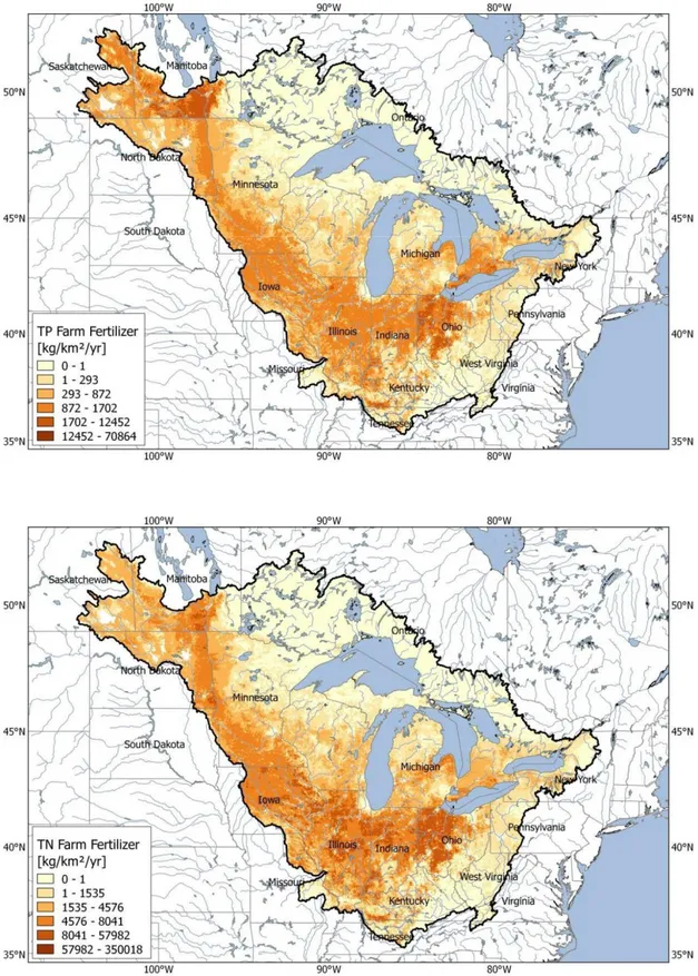
Fertilizer inputs in Canada were not available; therefore, fertilizer inputs needed to be estimated for this area. In the process of quantifying fertilizer inputs for the RA SPARROW model, Jenkinson and Benoy (2015) worked with AAFC staff to obtain the necessary data. A similar approach was used to estimate fertilizer inputs to the catchments in Canadian GL and WR basins from 2001 Census of Agriculture (Agriculture and Agri-Food Canada, 2002; 2007) data by census divisions (CD) and census consolidated subdivisions (CCS) that are a subset of CD. The CCS data provided greater resolution and were used where available, otherwise CD data were used. Appendix C provides further detail for calculating fertilizer loadings using these data. Once calculated, as with the U.S. county data, Canadian data were allocated to each SPARROW catchment by the fraction of the total agricultural land in the CD or CCS (Figure 12).

(34)

Figure 12: Total phosphorus (above) and total nitrogen (below) input rates, by catchment, throughout the Midcontinental region.

(35)

7.1.3 Manure

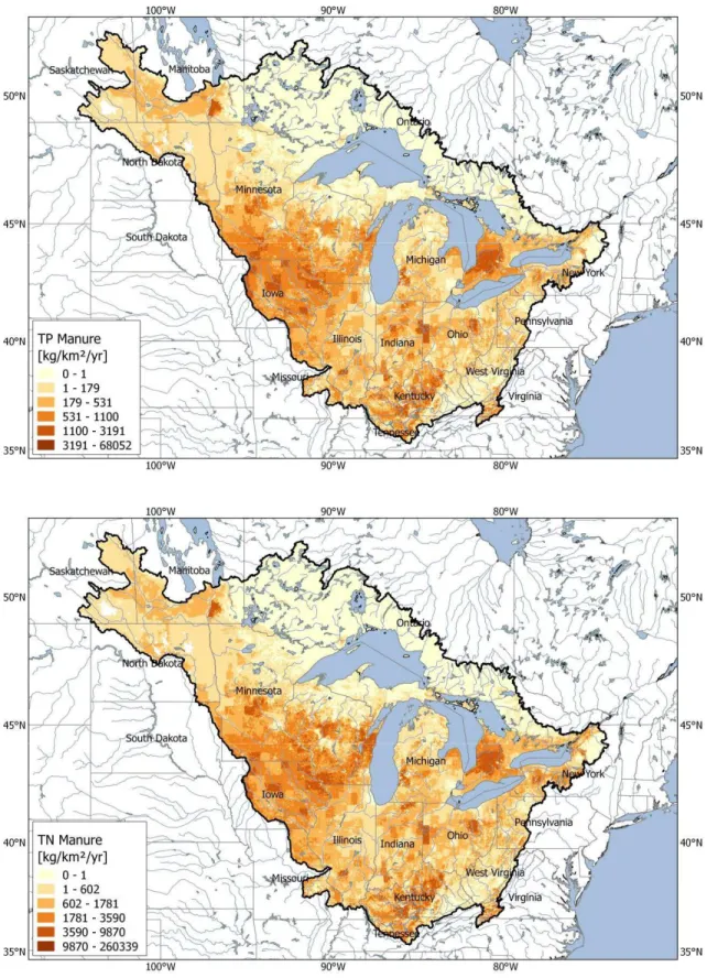
Livestock head counts are collected in both U.S. and Canada. A cross-walk table was devised to harmonize common classes of livestock between the U.S. and Canada data following Jenkinson and Benoy (2015) (provided in Table C-3 Appendix C). Livestock head counts were then multiplied by P and N coefficients for each animal type based on production rates (Ruddy et al., 2006) (provided in Table C-4 Appendix C). Total calculated manure was allocated to each SPARROW catchment based on the fraction of the agricultural and pasture land in the catchment (i.e., agricultural land and pasture class as defined in the land-cover layer). Livestock head counts by county in the U.S. and by sub-sub drainage area (SSDA) from the Interpolated Census of Agriculture (Agriculture and Agri-Food Canada, 2001) in Canada were used to allocate the P and N from manure. Where SSDA data were suppressed, as explained in Appendix C, 2001 Census of Agriculture (Agriculture and Agri-Food Canada, 2002; 2007) data by CD were substituted. For more information refer to Table C-5 Appendix C. County-level head counts from the 2002 Census of Agriculture (National Agriculture Statistics Service, 2004; Mueller and Gronberg, 2013) were used for the U.S portion of the model area. The N and P input rates from manure, by catchment, throughout the Midcontinental region are shown in Figure 13.

(36)

Figure 13: Total phosphorus (above) and total nitrogen (below) input rates, by catchment, from manure spread on agricultural and pasture lands throughout the Midcontinental region.

(37)

7.1.4 Atmospheric deposition

In previous SPARROW models developed for the U.S., atmospheric deposition was a significant contributing factor to TN loading (Robertson and Saad, 2011). For the Midcontinent SPARROW models, atmospheric deposition of N (a sum of wet and dry deposition) were estimated from the Community Multiscale Air Quality Modeling System (CMAQ) annual deposition rates for 2002 (Schwede et al., 2009; Hong et al., 2011; U.S. Environmental Protection Agency, 2018). Two different resolutions were employed (12 km and 36 km); 12-km resolution was used where available. The 36-km resolution data were used to supplement any missing regions, primarily in the northern reaches of the Midcontinental region. Atmospheric deposition rates of N throughout the Midcontinental region are shown in Figure 14.

Figure 14: Atmospheric deposition rates of total nitrogen from CMAQ, by catchment, throughout the Midcontinental region.

(38)

7.1.5 Wastewater-treatment plant inputs

P and N inputs from wastewater-treatment plants (WWTPs) throughout the Midcontinental region were based on effluent data for the U.S. and Ontario, and population estimates for Manitoba and Saskatchewan. For the U.S., 2002 annual WWTP effluent loads were calculated for each facility using monthly effluent flow and constituent concentration data from the USEPA Permit Compliance System national database (Robertson and Saad, 2011; Maupin and Ivahnenko, 2011). Effluent flow data were readily available for each facility; however, TN and TP concentration data were often unavailable (TP concentration data were more readily available than TN data). In cases where effluent concentration data were not available, effluent loads were estimated using typical pollutant concentrations (TPCs) based on the type and size (relative to effluent flow) of a facility, following methods described by Maupin and Ivahnenko (2011).

For Ontario, 2002 annual WWTP effluent loads were calculated using monthly flow and concentration data provided by the Ontario Clean Water Agency and Ministry of the Environment and Climate Change (personal communication, Antonette Arvai, 2013). Similar to the U.S., TP concentrations were occasionally and TN concentration data were frequently not available for some facilities in Canada. In such cases, TP and TN TPCs were generated based on either median concentration by facility treatment level (primary, secondary, tertiary or lagoon), or overall median concentration when facility treatment level information was missing (Table 1). Median concentrations were based on available data for 2002 through 2011.

Table 1: Median TP and TN WWTP effluent concentrations for Ontario, 2002 through 2011

Constituent Overall Primary Secondary Tertiary Lagoon

Median Concentration, mg/L (overall and by treatment level)

TP 0.3 0.76 0.37 0.13 0.26

TN 13.6 16.4 14.3 16.0 6.7

For WWTPs in Ontario, effluent records were identified as continuous or seasonal in the database. Facilities identified as continuous occasionally did not have all 12 months of flow and concentration data. For these sites, monthly loads were first calculated using the available monthly flow and concentration data and summed. Annual loadings were then computed by scaling up measured loads by the fraction of the year represented by available data. For example, if a facility had 9 months of available load data, the annual load was calculated as a sum of monthly loads multiplied by 1.33 (or 12/9). For seasonal facilities with missing monthly data, annual loads were calculated as the sum of available monthly loads.

Estimates of TP and TN loads from WWTPs in Manitoba and Saskatchewan were obtained from the MCWS, the Saskatchewan Ministry of Environment and the Saskatchewan Water Security Agency (personal

communication, Elaine Paige, 2013). Data in the RA basin were compiled for the RA SPARROW model area by Jenkinson and Benoy (2015). Data in the Manitoba region of the WR basin were compiled by Bourne et al. (2002). Effluent loads were calculated using 2008 population estimates and removal efficiencies based on facility treatment levels (Chambers et al., 2001). Influent loads were calculated from the number of people served by the facility multiplied by 1.23 kg per person per year for TP and 3.65 kg per person per year for TN (Chambers et al., 2001). Effluent loads were calculated as the influent load multiplied by 1 minus the removal efficiency, which ranged from 0.59 to 0.66, depending on the facility treatment level.

Locations of the WWTP facilities are shown in Figure 15. The locations of the all facilities in the U.S. and Canada were visually inspected using aerial photographs and confirmed where possible. WWTP inputs were summed for each SPARROW catchment based on the facility locations.

(39)

Figure 15: Wastewater-treatment plants used in the Midcontinent SPARROW models.

7.1.6 Non-modeled contributing areas

The Qu’Appelle River in Saskatchewan and Missouri River in central U.S. contribute P and N to the Midcontinental region; however, neither basin is explicitly included in the region. Difficulties in developing a digital stream network for the Qu’Appelle River prevented inclusion of its area. The Missouri River was

excluded in an effort to limit the size of the modelled area. To account for the P and N inputs from these rivers, the estimated long-term mean annual TP and TN loads from these areas were input as point sources at the location in the digital stream network that represents the confluence with the non-modeled areas. The long-term mean annual loads for the Missouri River (Station ID 06934500; TP=28,220,000 kg/yr; TN=195,900,000 kg/yr) were estimated using the computer program Fluxmaster (Schwarz et al., 2006), similar to the loads used for the regional SPARROW models (Saad, et al., 2011). The long-term mean annual loads for the Qu’Appelle River (Station ID SA05JM0014, TP=67,880 kg/yr; TN=472,700 kg/yr) were estimated using a newer version of the computer program Fluxmaster following methods described in Saad et al. (2018).

(40)

7.2 Delivery variables

Delivery variables in SPARROW describe properties of the landscape that relate to climatic, natural or anthropogenic terrestrial processes affecting contaminant transport from the land to the stream. The following delivery variables were examined for inclusion in the Midcontinent SPARROW models:

• climate (i.e., precipitation, air temperature and runoff), • soil characteristics,

• mean catchment slope, and • tile drainage.

7.2.1 Climatic data

Climatic data, such as air temperature and precipitation, have been shown to be significant variables in earlier SPARROW modelling studies (Robertson and Saad, 2011; 2013). Runoff was another variable considered for this category because it represents a direct delivery method from land to water relying on climatic data, such as air temperature and precipitation.

Air Temperature

For the U.S. portion of the Midcontinental region, mean annual air temperature data (30-year normals from 1971 to 2000) were obtained from the Parameter-elevation Regressions on Independent Slopes Model (PRISM) Climate Group (PRISM Climate Group, 2006). PRISM data are comprised of average values at the end of each decade over a 30-year period. For the Canadian portion of the region, air temperature data collected by the Canadian Forest Service (CFS) (McKenney et al., 2006) were used. CFS temperature data consist of minimum and maximum temperature grids, whose values were reprocessed as defined in (McKay et

al., 2012) to ensure congruity between U.S. and Canada. Mean annual temperatures throughout the

Midcontinental region are shown in Figure 16.

(41)

Precipitation

Mean annual precipitation rates for the entire region were obtained from Canadian Precipitation Analysis (CaPA) (National High Impact Weather Laboratory, 2014) data. Jenkinson and Benoy (2015) demonstrated that CaPA data were seamless across the U.S. – Canada border. The CaPA data for the Midcontinent SPARROW models were obtained from ECCC (personal communication, Bruce Davison, March 27, 2015). Data were provided in 6-hour time-steps, covering years 2002 to 2010, which were accumulated on an annual basis and calculated to 9-year mean annual values. The original grid cell resolution was provided in 10 km, with

precipitation provided in units of metres. Mean annual precipitation throughout the Midcontinental region is shown in Figure 17.

(42)

Runoff

Runoff is controlled by climatic variables, such as precipitation and air temperature and by basin

characteristics, such as slope and soils. Mean annual runoff covering the entire Midcontinental region was estimated using the Wolock and McCabe (1999) water balance model. U.S. data was obtained from Wolock and McCabe (2018). Canadian runoff data were computed from the PRISM and CFS data described in the Air Temperature discussion above. Mean annual runoff throughout the Midcontinental region is shown in Figure 18.

(43)

7.2.2 Soil characteristics

Variability in soil characteristics throughout the Midcontinental region were described using soil permeability and clay content. For the U.S. portion of the Midcontinental region, these datasets came from the Natural Resources Conservation Service State Soil Geographic (STATSGO) database (Schwarz and Alexander, 1995; U.S. Department of Agriculture, 1994; Wolock, 1997; Wieczorek and LaMotte, 2010). Data for the Canadian portion of the region were estimated with assistance by AAFC. Unlike for the provinces of Saskatchewan and Manitoba, soil permeability data for the province of Ontario were incomplete. Soil Landscape of Canada data version 2.2 (Agriculture and Agri-Food Canada, 1996) were reprocessed by AAFC (personal communication, Glenn Lelyk, 2015–2017) to be consistent with the U.S. data. To harmonize U.S. and Canadian data, the Canadian data were adjusted to the STATSGO soil permeability scale (0.06, 0.13, 0.4, 1.3, 4, 13, and 20 in/hr) where available. In areas where data were unavailable (primarily north of Lake Superior, Lake Huron and Georgian Bay), soil characteristics were estimated based on neighbouring data and a basic understanding of the geology in the area. This method provided less spatial detail than data used in the SPARROW models by Jenkinson and Benoy (2015) and Robertson and Saad (2011), but resulted in consistency over the full Midcontinental region. The final soil permeability and clay content distributions are shown in Figure 19.

(44)

(45)

7.2.3 Mean catchment slope

Three different DEMs were used to calculate mean catchment slopes throughout the Midcontinental region. The NED DEM (Gesch et al., 2002) was used for the U.S. portion of the region and the WR basin. The Canadian Digital Elevation Dataset (CDED) was used for the RA basin (Jenkinson and Benoy, 2015). The OIHD DEM (Ontario Ministry of Natural Resources and Forestry, 2012) was used for the Canadian portion of the GL basin. The NED and OIHD DEMs had a horizontal resolution of 30 m, while the CDED (Centre for Topographic Information, 2000) had a horizontal resolution of 15 m. For those catchments where calculations resulted in zero or negative slopes, a value of 0.00001 was enforced to avoid calculation errors in the

SPARROW model. Mean catchment slopes throughout the Midcontinental region are shown in Figure 20.

(46)

7.2.4 Tile drainage

Robertson and Saad (2011) have shown, using SPARROW models, that the amount of area drained by tiles may affect the delivery of P and N to streams. Tile drainage data for the U.S. portion of the region were based on early 1990s information compiled by Nakagaki et al. (2016) following methods described by Sugg (2007). This information was processed to NHDPlus catchments using methods described by Wieczorek et al. (2016). For the Canadian portion of the region, tile drainage data of various forms were available at a provincial level. The Ontario Ministry of Agriculture, Food and Rural Affairs (OMAFRA) collects data describing tile drainage within the province and provides the information in the dataset Tile Drainage Area (Ontario Ministry of Agriculture Food and Rural Affairs, 2015). This information is available at a horizontal resolution of approximately 500 m and does not provide precise representations of the area drained. The assembled information provides the location and, in some cases, the size of installed tile drains. Areas with tile information were well represented as of 1983, when reporting and data collection commenced. Manitoba Sustainable Development (MSD) maintains a database describing tile drainage throughout the province based solely on location (personal communication, Tara Wiess, Manitoba Sustainable Development, 2016). Saskatchewan has historically been relatively arid, with only recent annual precipitation exceeding 500 mm. As a result of these arid conditions, tile drains have rarely been used in the province. Consequently, relevant information is deemed too insignificant to collect from Saskatchewan (personal communication, Doug Johnson, 2016); therefore, tile drains were assumed to not be present throughout this province.

Tile data for Ontario were processed for locations installed prior to and including 2002 (which resulted in approximately 74,000 records). Within this dataset, all of the records were provided as polygon features, but only 720 records had attribute information that had both polygon size and the area with tile drains. Therefore, to assess tile drainage in Ontario, installed drain-size area data from the 720 records with detailed data were used to obtain a relationship between polygon size and the area with tile drains. This relation was then used with polygon surface area to obtain information for all 74,000 areas with tile drains.

Tile drain locations in Manitoba were provided as a point feature by MSD. A total of 912 records existed, but only 28 had attribute information describing the area with tile drains. A dataset describing tile drainage areas in North Dakota (Finocchiaro, 2016) was used to improve the usefulness of the Manitoba data. The median tiled area for each location with North Dakota’s tile data was calculated (0.615 km2_{) and applied as a factor to each}

Manitoba point location already provided. For both Ontario and Manitoba, the amount of tiled area in each catchment was summed and the percentage of each catchment underlain by tiles was calculated resulting in data similar to that compiled for the U.S. The percentages of each catchment underlain with tile drains are shown in Figure 21.

(47)

Figure 21: Percentage of the catchment underlain with tile drains, by catchment, throughout the Midcontinental region.

(48)

8 Summary

SPARROW models require extensive and contiguous geospatial datasets describing the stream network, catchments, nutrient inputs, and environmental variables affecting the transport of nutrients to the streams, and transport throughout the stream network. Using the data and procedures described in this report, a harmonized digital stream network was developed with information describing waterbodies and streamflow along the network. The stream network was used to create catchments (~2.5 km2_{) throughout the Midcontinental region}

of North America. Various geospatial datasets describing phosphorus and nitrogen inputs to each of the catchments (for conditions similar to 2002) and landscape characteristics that potentially describe variability in the delivery of nutrients to streams were assembled and harmonized across the U.S. – Canada border. The phosphorus and nitrogen inputs and landscape characteristics were then geospatially allocated to each of the catchments throughout the Midcontinental region. All of the nutrient input data, delivery data, and stream and reservoir data can be used to develop total phosphorus and total nitrogen SPARROW models for the

Midcontinental region of North America. All of these data are available for download at url: https://doi.org/10.4224/300.0001.