Pressure, surface tension, and curvature in active
systems: A touch of equilibrium
René Wittmann,1,2,a)
Frank Smallenburg,2,3
and Joseph M. Brader1
1Department of Physics, University of Fribourg, CH-1700 Fribourg, Switzerland
2Institut für Theoretische Physik II, Weiche Materie, Heinrich-Heine-Universität Düsseldorf, D-40225 Düsseldorf, Germany 3Laboratoire de Physique des Solides, CNRS, Univ. Paris-Sud, Univ. Paris-Saclay, Orsay, France
a)Electronic mail:[email protected]
ABSTRACT
We explore the pressure of active particles on curved surfaces and its relation to other interfacial properties. We use both direct simulations of the active systems as well as simulations of an equilibrium system with effective (pair) interactions designed to capture the effects of activity. Comparing the active and effective passive systems in terms of their bulk pressure, we elaborate that the most useful theoretical route to this quantity is via the density profile at a flat wall. This is corroborated by extending the study to curved surfaces and establishing a connection to the particle adsorption and integrated surface excess pressure (surface tension). In the ideal-gas limit, the effect of curvature on the mechanical properties can be calculated analytically in the passive system with effective interactions and shows good (but not exact) agreement with simulations of the active models. It turns out that even the linear correction to the pressure is model specific and equals the planar adsorption in each case, which means that a known equilibrium sum rule can be extended to a regime at small but nonzero activity. In turn, the relation between the planar adsorption and the surface tension is reminiscent of the Gibbs adsorption theorem at an effective temperature. At finite densities, where particle interactions play a role, the presented effective-potential approximation captures the effect of density on the dependence of the pressure on curvature.
I. INTRODUCTION
Recent advances in colloidal science have allowed for the cre-ation of active colloids: synthetic particles which are capable of using energy from their environment to fuel active self-propelled motion.1–3Due to their constant motion, systems of active particles are inherently out-of-equilibrium and, hence, do not follow the usual rules of equilibrium thermodynamics. The emergence of activity has spurred a new interest in the statistical physics of such systems.4,5 A topic of particular interest is the question of whether equilib-rium concepts, such as pressure,6–8interfacial or surface tension,9–11 chemical potential,12–14temperature,15,16and free energy,12,17,18can be extended to provide meaningful insights into active systems as well. Of these quantities, the active pressure has perhaps been scru-tinized the most. In its most simple definition, the pressure can be identified with the force per unit area the active particles exert
on the confining walls. Unlike in equilibrium, this force gener-ally depends not only on the bulk properties but also on the wall-particle interaction,7preventing the definition of a bulk pressure in this way.
The standard model system of active Brownian particles (ABPs) consists of particles, which propel themselves with a constant veloc-ity along their instantaneous orientation, subject to rotational Brow-nian motion. Such ABPs interact with each other and the wall only via isotropic interactions. In this special case, the pressure has been shown to be a state function, which provides one condition to pre-dict coexistences between different phases, analogous to the equilib-rium pressure.19This means that the pressure that a fluid of ABPs exerts on a flat wall is simply equal to the bulk pressure, regard-less of the wall–particle interaction. However, if the wall is curved, it is not obvious how the force per unit surface area is related to the active bulk pressure. Indeed, simulations have shown that, even for a
http://doc.rero.ch
Published in "The Journal of Chemical Physics 150(17): 174908, 2019"
which should be cited to refer to this work.
noninteracting active gas, the active pressure of ABPs strongly depends on the wall curvature20 and follows the structure of the wall in a local fashion.21This observation can be explained by con-sidering regions of a highly negative (positive) curvature as cavi-ties (obstacles), which lead to an increased (decreased) probability of finding a particle near the wall and thus a higher (lower) con-tribution to the wall pressure compared to its bulk value. Here and throughout this paper, we use the convention that the surface normal points toward the bulk.
Neglecting all autocorrelation functions of the self-propulsion force beyond the second order, the activity of ABPs can be approx-imately represented by colored noise.22 These active Ornstein-Uhlenbeck processes (AOUPs) constitute another example for an isotropically interacting model system, in which the self-propulsion vector fluctuates in both the direction and length. In a man-ner of speaking, AOUPs are even more simplistic and closer to equilibrium23 than ABPs, as their motion reverts to simple overdamped Brownian dynamics in the limit of short correla-tion time (without addicorrela-tionally introducing a Brownian thermal noise). Although there are, in general, some important differences between the two model systems,16,24–26 many essential aspects of the nonequilibrium behavior of ABPs and AOUPs are quite simi-lar. For example, recent results concerning the pressure of AOUPs at curved walls27,28 qualitatively reproduce the observations for ABPs.21
The AOUPs model is also known for being a convenient start-ing point to develop an effective description of active systems by means of their configurational probability distribution, allowing us to exploit techniques familiar for (near) equilibrium systems.22,29–33 As a possible second step to this equilibrium mapping, the effective-potential approximation (EPA)17,22,32,34–36 has been employed to construct a closed theory to study the active system, e.g., using vari-ational methods. The crucial idea of this approximation is to derive a pairwise-additive effective interaction force to represent the activ-ity within a framework developed for passive systems. This proce-dure is even possible if the two particles considered have different activities.37
The basic idea of representing active particles by equilibrium ones has an ambiguous taste. On the one hand, the simplicity of the time-evolution equation allows for the construction of partic-ularly simple theories; on the other hand, many inherently out-of-equilibrium aspects cannot be accounted for in this way. Nev-ertheless, this approach was proven to be quite useful in several situations since some steady-state results can be accurately repro-duced in systems with low activity and spatial dimensionality.34,35 In the small-activity limit, the effective equilibrium mapping recov-ers several exact results for an ideal gas.37,38 For interacting parti-cles, some closed formulas for the mechanical properties have been derived,31,36which are consistent with the concepts of swim pres-sure6and active interfacial tension.9In addition, the EPA provides a solid qualitative understanding of the phase behavior of inter-acting active systems.17,22 Recently, the effective equilibrium rea-soning has been adopted for other models39and some alternative approaches have been proposed to obtain improved one-body dis-tribution functions.40,41A quantitative description of active particles in effective equilibrium is, however, usually difficult, in particular, when it comes to a calculation involving the pair correlations in an interacting three-dimensional system.32A related argumentation in
a different context expounds that the predictions of an approximate theory become worse if the results are obtained via two-point instead of one-point distributions.42
Another important question related to the applicability of the EPA concerns the role of curvature, which emerges in two dis-tinct types. First, the notion of a potential curvature describes the change of slope of a soft potential landscape, i.e., the change of magnitude of the external force, in a certain direction. It has been concluded in the context of various one-dimensional problems that most accurate results can be obtained for a small absolute value of the potential curvature.33,40,41 Second, in higher spatial dimen-sions, the shape of a hard wall or particle can be characterized by its geometrical curvature. More generally, one can also refer to a characteristic equipotential line when the interaction is soft. The first proper prediction of the qualitative dependence on the geo-metrical curvature is that a larger number of active ideal particles accumulate in a cavity than at an obstacle.30Later, an explicit ana-lytic result has been obtained for the density of particles trapped in a cavity.25In this case, the theory has been confirmed to become exact in the limit of an infinite persistence time, which has been reported to be generally the case in one dimension.43,44At an obsta-cle or for interacting partiobsta-cles, where the geometrical curvature is positive, the EPA cannot be employed properly without an empirical correction.35
In this paper, we address the issues outlined above specific to the EPA17,22,25,29–31,33–36 in more detail and in the context of a well-studied property of active particles, namely, their pressure. Explicitly, we are concerned with the fundamental questions: (i) how accurately can we predict the active pressure in the presence of interparticle interactions, (ii) to what degree can the peculiar behavior of active particles at curved20,27,28or structured21,28surfaces be captured, (iii) does the (corrected) theory also provide proper results for a positive geometrical curvature, and (iv) what is the relation between the pressure and the surface excess properties at the wall? We corroborate our theoretical findings by performing computer simulations of active systems. To allow for a quantita-tive comparison, we go beyond approximate theories to implement the EPA by performing explicit simulations of the effective passive system. We conduct our study in two dimensions since the accu-racy of the effective potentials is known to decrease with increas-ing dimensionality.35 Moreover, in two dimensions, overdamped models of active particles, which ignore hydrodynamic interac-tions, are more realistic since a substrate can act as a momentum sink.
The remainder of this paper is arranged as follows: In Sec.II, we briefly recapitulate the effective equilibrium model and the EPA35to the extent required here. We then compare in Sec.IIIactive and pas-sive simulations to measure the pressure of an interacting system in the bulk and on a flat wall. In Sec.IV, we consider active ideal gases near curved walls and describe at small activity (or curvature) the relations between active pressure (excess), adsorption, and surface tension (or, more accurately, the negative integrated surface excess
pressure),45reminiscent of equilibrium sum rules.46Moreover, we
extract the leading-order curvature correction to the pressure in the presence of interactions. We conclude in Sec.V on the perspec-tive of the employed equilibrium mapping and the relation between bulk and surface excess properties in active systems with isotropic interactions.
II. EFFECTIVE EQUILIBRIUM THEORY
In the following, we briefly introduce the main results of the EPA required to later calculate the mechanical pressure. Throughout the paper, we assume that in the active system, there is no transla-tional thermal noise, which would be necessarily present in a pas-sive Brownian system, and are only interested in the steady-state behavior. Then both schemes, based on the one-dimensional Fox approach47and Unified Colored Noise Approximation,44to develop a generalized equilibrium mapping for the multicomponent system in an arbitrary dimension are equivalent.35 The reader interested in the full derivation and further technical details is referred to the extensive literature on this subject, in particular, Refs.22,29, and35. The related microscopic equations of motion of ABPs and AOUPs are explained inAppendix A.
In effective equilibrium, we consider an active system whose steady-state configurational probability distribution PN(rN) solves
the equation35 βFiPN− N ∑ j ∇j(DjiPN) = 0 , (1)
where β= (kBT)−1is the inverse of the temperature T with
Boltz-mann’s constant kB. Note that in the absence of thermal noise, β
here simply functions as an (activity-independent) inverse energy unit, whose choice does not affect the behavior of the system. More-over,Fi(rN) represents the conservative force on particle i and the
dimensionless effective diffusion tensorDij(rN) serves to represent
the activity of the N particles of diameter d and equals unity in the passive case. Explicitly, it depends on the persistence time τaof the
self-propelled motion and its magnitude. The latter is characterized by the active diffusivity Da(in the case of AOUPs) or by the
con-stant self-propulsion velocityv0(for ABPs), where, in two
dimen-sions, we can identify both parameters according to the relation
Da= v02τa/2. For later convenience, we also introduce the persistence
length lp∶=√2Daτa= τav0of the active motion.
Explicitly, the components of the inverse ofDijread as35
D−1ij (rN) = D−1a (1δij− τd2∇iβFj(rN)), (2)
with the dimensionless persistence time τ = τa/τ0, where τ0= (βγd2)
denotes the damping time, and diffusivityDa = Daβγ, where γ
is the friction coefficient. Inspecting Eq. (2), we see that in the absence of external forces active particles experience an effective active temperature scale βeff= β/Dasince their diffusion is enhanced
byDa16 compared to a passive system, which is explicitly
recov-ered in the white-noise limit of the AOUPs model, τ → 0 while
Da= 1 is kept finite. This effective diffusion is reduced by
approach-ing a repulsive wall or when particles with repulsive interactions accumulate. While this intuition already reflects the behavior of active particles quite nicely in a dynamical picture, the versatility of the effective equilibrium approach comes from the possibility to describe the nonequilibrium steady states by means of a static for-mula, i.e., Eq.(1), which still depends on this (effective) diffusion tensor. As detailed later, its contribution results in an increase in effective attraction or a decrease in active pressure when the particles become more active. As a further consequence, the effective dynam-ics of active particles are described by a complex interplay of both the activity-dependent effective diffusion and modified force terms, which determine the effective equilibrium state. In fact, depending
on the chosen theoretical framework, a slightly different interpre-tation of the latter is necessary to specify a Fokker-Planck equation for the time evolution of PN, whereDij acts as a diffusion tensor:
the Fox approximation suggests the existence of an effective force,36 while the Unified Colored Noise Approximation results in an addi-tional contribution to the bare interaction force.30The explicit form of Eq.(2)is the same in both theories, as long as translational Brow-nian noise is negligible. Hence, the steady-state condition, Eq.(1), is identical and the two different interpretations of the force terms are formally equivalent so that we may choose the most convenient one.35
Returning to the static behavior, we solve as a first step Eq.(1)
for the effective equilibrium probability distribution PN. Then, we
can readily identify effective interaction potentials (seeAppendix B) accounting for the increase in probability to find a repulsive active particle near a boundary or another particle. Considering the case with N = 2 particles, we haveF1 =−F2=−∇u(r) with
the pair potential u(r). Then, we can define the effective pair potential βueff(r) =−ln P2. Likewise, from the interaction forceF1
=−∇v(r) of a single particle (N = 1) with an external one-body field one-body field v(r), we obtain βveff(r) = −ln P1. Notice that the
effective diffusion tensor in Eq.(2)is not always positive definite. As detailed inAppendix C, it may become negative for potentials with a negative potential curvature or a positive geometrical curvature. Hence, to be able to extend our study to the behavior of active parti-cles at obstaparti-cles in this work, we employ inAppendix Ban empirical modification, the inverse-τ approximation, which ensures qualita-tively correct behavior of effective potentials35even in such situa-tions. For a cavity, the effective diffusion tensor is always positive definite.
In order to make analytic progress, we follow Ref. 25 and choose a simple power-law dependence of the bare interaction potentials of the form∼λxn, introduced in full detail inAppendix B, with an integer-valued exponent n≥ 2 and a softness parameter λ, which ranges between 0 (no interaction) and infinity (hard interac-tion). The most handy potential, one branch of a parabola, results in a spurious discontinuity of the effective potentials at the posi-tion of the vertex25since the second derivative of a parabola does not vanish at the apex. Despite this artifact, it can be verified by choosing exponents n> 2 that the analytic results at a hard wall obtained in this way remain invariant. In order to avoid any pit-falls, all numerical calculations are carried out with the exponent
n = 4.
III. ACTIVE BULK PRESSURE
The pressure p(B)act in a torque-free active system can be
mea-sured in bulk8or from the force on a flat wall in a sufficiently large system, which we denote as p(W)act ≡ p(B)act. At the moment, the useful-ness of the EPA to calculate the active pressure is not quite evident. This is mostly due to the misjudgment that the desired quantity can be identified with the effective thermodynamic pressure peffobtained
from a standard equilibrium calculation for a passive system inter-acting with the effective potential βueff(r). For example, using the virial theorem, we have
βpeff= ρ0−π 2ρ 2 0∫ ∞ 0 dr r 2 g(r)∂βueff(r) ∂r , (3)
http://doc.rero.ch
where g(r) is the radial distribution function and ρ0is the bulk
den-sity. However, this effective pressure was explicitly shown not to share obvious attributes of a (mechanical) active pressure.32,36The reasons for this discrepancy have been discussed in Ref. 36, and an artificial rescaling was presented on a formal level (this rescaled pressure p(R) was argued to be inferior to the virial pressure p(V) introduced below). On the other hand, the EPA provides a con-venient theoretical route to access the radial distribution function of the active particles, which can be used as input for a closed virial-like expression to calculate the active pressure. Moreover, we will propose another, more intuitive way to calculate the pressure within the EPA by its force exerted on a planar (and later curved) wall.
Using the virial theorem, statistical formulas for the active pres-sure (and interfacial or surface tension) have been derived in Refs.31
and36, which depend solely on properties of the bulk fluid via the ensemble averageD(r) of the effective diffusion tensor Dij. We use
the approximate representation
DaD−1(r) ≈ 1 + τd2∫ dr′
ρ(2)(r, r′)
ρ(r) ∇∇βu(r, r
′) (4)
of this quantity, where ρ(2)is the two-particle density, which in the bulk becomes ρ(2)(∣r − r′∣) ≃ ρ20g(r). The choice of the expression
in Eq.(4)can be motivated in two ways. The first strategy involves an expansion up to linear order in the persistence time (low-activity approximation) to be able to carry out the ensemble average of
Dij31,35and replace this average with Eq.(4)to restore in the resulting
expressions the neglected higher-order terms. The second approxi-mation amounts to rederive the virial formulas in a more indirect way, which allows us to explicitly take the average of the inverse diffusion tensor, i.e., Eq.(2).35,36
To apply the virial theorem to the equality in Eq.(1), we sepa-rate the force in an external part representing the boundary and an internal force due to particle interactions. Then, the virial pressure of an active bulk system follows in two dimensions as31,36
βp(V)=Tr[D] 2 ρ0− π 2ρ 2 0∫ ∞ 0 dr r 2 g(r)∂βu(r) ∂r . (5)
The second term equals the passive virial, compare Eq.(3), and only depends implicitly on the activity through changes in the (effective) radial distribution g(r) compared to a passive system. The trace in the first term can be written as
Tr[D] = 2Da 1 + πρ0τd2∫ dr r g(r)(∂ 2βu(r) ∂r2 + 1 r ∂βu(r) ∂r ) = 2Da 1 +⟨τdN2∑i<j(∂ 2βu(r ij) ∂rij + 1 rij ∂βu(rij) ∂rij )⟩ (6)
since we consider a homogeneous and isotropic system. The deriva-tion of Eq.(5) circumvents the definition of effective interaction potentials. Therefore, the expression for p(V) can also be used together with the radial distribution obtained from computer simu-lations of a true active system. In this case, we write p(V)act, whereas p(V)
corresponds to a calculation within the EPA. Note that the bulk pres-sure p(B)act is also obtained from a virial-based approach8but should
not be confused with the approximate expression for p(V)act and that it is not possible to determine an expression in the EPA that is analog to p(B)act.
Apart from the bulk route, we now consider an active fluid at a planar wall characterized by the bare external potential v(x). For such a setup, we can deduce the mechanical pressure
βp(W)= − ∫ ∞
−∞dx
∂βv(x)
∂x ρ(x) (7)
from its most fundamental definition: the force per unit area exerted on a wall. Again, the inhomogeneous one-body density ρ(x) can readily be measured for an active system, yielding p(W)act, or for a pas-sive system within the EPA, where we write p(W). In the latter case, it is important to determine ρ(x) for the effective wall with veff(x) although the pressure is then measured with the help of v(x). For isotropically interacting active particles, which we aim to describe here, p(W)act is independent of the wall potential19,21and, hence, equal
to p(B)act. Therefore, we set pact≡ p(W)act ≡ p (B)
act. For an active ideal gas, all
expressions βp(W)= βp(V)= βp(W)act = βp (V) act = βp (B) act= Daρ0 (8)
yield the exact ideal swim pressure.36Apparently from Eq.(3), the effective thermodynamic pressure βpeff= ρ0, on the other hand, is
independent of both activity and the wall-particle interaction. In general, there exists no trivial relation between p(W)and peff.
Inspired by the equivalence in Eq.(8)for an ideal gas, it is instruc-tive to multiply the effecinstruc-tive pressure withDa, i.e., switching to the
effective temperature scale βeff. To make the connection with Eq.(7),
we replace v(x) with the effective external potential veff(x) and define the effective-temperature pressure
βp(T)= −Da∫
∞
−∞dx
∂βveff(x)
∂x ρ(x) ≡ βeffpeff (9)
for a flat wall and a sufficiently large system. The latter equality fol-lows from the wall theorem of equilibrium thermodynamics, which holds for any interacting passive fluid if the calculation can be done exactly. Alternatively, peffcan equally be determined via Eq.(3). By
construction, the correct (active) ideal-gas solution βp(T) = Daρ0is
also recovered from Eq.(9). Since this definition explicitly makes use of an EPA result (veffor peff), there is no sensible equivalent for the
full active system.
A. Interacting particles at a flat wall
In order to better assess the accuracy of the EPA, we now extend the comparison from Ref. 36of the different routes to calculate the active pressure by (i) implementing the effective pair potentials numerically in a passive simulation to circumvent the need for fur-ther approximations, (ii) additionally considering the expressions
p(W)and p(T)proposed in Eqs.(7)and(9), respectively, for the pres-sure from the force of a wall, and (iii) including different active computer simulation results as a reference, where we (iv) also test the general value of Eq.(5)for an active system by calculating p(V)act. Also recall that in the present study, we focus on two-dimensional systems. In all simulations, we fix the self-propulsion speed of the particles v0= 24d/τ0, while changing their persistence time τ and
hence the associated persistence length lp. An increase in τ thus
represents an increase in activity.
InFig. 1, we show the active pressure as a function of the den-sity for different activity parameters and compare it to pressures measured in the corresponding passive system with effective inter-actions. For ABPs and AOUPs, we measured both the bulk pres-sure p(B)act in a system without walls (using the virial expression in Ref.8) and the mechanical pressure p(W)act on a flat wall in a suf-ficiently large system. As expected, p(B)act = p(W)act in all cases, repre-senting the true pressure pactexerted by the active particles on their
container. Moreover, we find essentially the same active pressures for the ABPs and AOUPs models for all investigated activities and
FIG. 1. Comparison between different methods for determining the active pressure of bulk systems as a function of the bulk density ρ0and for different rotational
diffu-sion times (a) τ = 0.005, (b) τ = 0.01, (c) τ = 0.025, and (d) τ = 0.05. In all cases, the self-propulsion speed is fixed atv0= 24d/τ0. The points represent
measure-ments performed directly in simulations of ABPs or AOUPs, and lines indicate the EPA pressures measured in a passive system with effective pair interactions. The label pactcollects the equivalent reference results for p(B)actand p
(W)
act. For τ = 0.05,
the passive system phase separates at densities ρ0d2≳ 0.5.
densities. By contrast, the pressure p(V)act derived from the effec-tive diffusion tensor is approximate and increasingly deviates from the true bulk pressure as activity increases for both the ABPs and AOUPs models.
For the corresponding passive systems, we also plot inFig. 1
the pressures p(V), p(W), and p(T)using Eqs.(5),(7), and(9), respec-tively. The theoretical pressures p(W), calculated from the bare poten-tial v(x), and p(V)act, calculated from the effective diffusion tensor,
exhibit a similar behavior at low activity τ ≲ 0.01, whereas the (rescaled) thermodynamic pressure p(T) of the passive system is always larger. At higher activities, there are significant differences between the three theoretical methods and, quite surprisingly, p(T) follows the true pressure pact much more closely, even at higher
densities. Significant deviations only occur for strong activity τ ≳ 0.05, where the passive system undergoes a phase separation for densities ρ0d2 ≳ 0.5 and, hence, pressures can only be
reli-ably calculated up to that density. This phase transition shifts to lower densities when further increasing τ.17,22 Also the agreement between p(W)and pactremains reasonable at low densities or small
activities.
Comparing the results of the virial pressures p(V)of the pas-sive system (calculated using the bare interparticle potential) and
p(V)act of the active system, we find good agreement in all cases where
phase separation does not occur. Since these are both calculated from the radial distribution function g(r), this observation suggests that the approximations involved in deriving Eq.(5) are cruder than those leading to the approximate radial distribution g(r) within the EPA. To check this, we compare g(r) for different parameters inFig. 2, which illustrates the known deviations at higher densi-ties and actividensi-ties although the agreement remains reasonable at all parameters considered. Such a comparison has already been done
FIG. 2. Comparison of the radial distribution function g(r) in the passive and active system, for different persistence densities ρ0as indicated, at fixed self-propulsion
velocityv0= 24d/τ0. The persistence times are (a) τ = 0.005 and (b) τ = 0.025.
in three dimensions and with another approximation for the effec-tive potential, where the disagreement was shown to be much more severe,22,32 whereas in one dimension, no further approximation becomes necessary and an even better match between theory and simulations was found.34We again find virtually identical results for
g(r) in the ABPs and AOUPs models and good agreement with the
EPA model.
Finally, we observe inFig. 1a small horizontal offset between the points corresponding to the active pressure pactof AOUPs and
ABPs simulated at the same particle number and volume, especially at high activity. These systems were simulated in the presence of two flat walls; hence, this shift results from a difference in the observed bulk densities caused by a difference in the adsorption at the wall between these two models. This is intriguing as the bulk pressures and radial distribution functions of the two models are essentially the same for all densities and activities. Evidently, while ABPs and AOUPs behave identical in the bulk, they show significant differ-ences in their behavior near a wall. This observation will be quanti-fied and extended in Sec.IV, where we consider more general sys-tems with curved walls for which the flat-wall results are recovered in the zero-curvature limit.
IV. CURVATURE DEPENDENCE
Having verified that the active pressure in the EPA is best cal-culated by the force exerted on a wall, we still need to answer the question whether the effective-temperature pressure p(T), defined in Eq.(9), is superior to the more realistic mechanical pressure p(W) from Eq.(7)also in more general situations. The logical next step is thus to consider curved surfaces, focusing on a circular geometry of radius R for the moment. To distinguish a cavity (particles inside the circle) from an obstacle (particles outside the circle), we have to consider two different potentials v−(r) and v+(r). These expres-sions, as well as the corresponding effective potentials veff∓(r), for-mally become equivalent in the limit R→ → ∞ of a planar wall; seeAppendix B. Following the convention of Ref.20, we formally consider a signed curvature radius R, which becomes negative for a cavity, to represent the corresponding wall by a negative geometrical curvature; seeAppendix Cfor more details. We denote the respec-tive pressures p(W−)(R−1) for a cavity with R< 0 and p(W+)(R−1) for an obstacle with R> 0 by a modified superscript. With these adjust-ments, the overall pressure p(W)(R−1) is a continuous function where the planar limit p(W)(0) = p(W)is given by Eq.(7). The same applies to all other quantities considered.
A. Pressure, adsorption, and surface tension
Calculating the total force on the area (circumference)
A = |2πR| of a circular wall of radius R with the convention described
above, the two contributions to the pressure p(W)(R−1) become
βp(W∓)(∣R−1∣) = ± ∫ ∞ 0 dr r R ∂βv∓(r) ∂r ρ(r) (10)
and equally for p(W)act (R−1) if ρ(r) is measured in the active systems.
The argument |R−1| serves to emphasize that we evaluate the right-hand side for the absolute value of R, which appears in the potentials specified inAppendix B. To obtain the correct result as a function of
the signed curvature R−1, we later change the sign of R in the formu-las with superscript (−) for a cavity. The corresponding expressions for βp(T∓)(∣R−1∣) = ±Da∫ ∞ 0 dr r R ∂βveff∓(r) ∂r ρ(r) (11)
in the passive system simply follow from replacing v(r) with
Daveff(r) in Eq.(10).
It is instructive to further consider some (mechanical) excess properties at the surface. Equivalent to the surface excess grand potential in statistical mechanics for a passive system,46we define mechanically the total surface tension45 (or, more accurately, the negative integrated excess pressure) of a fluid at a circular surface as
σ(∓)(∣R−1∣) = ∫ ∞
0 dr
r
R(p Θ(∓(r − R)) − pT(r)) , (12)
where we locate the surface at the apex (r = R) of the wall potential,
p denotes the bulk pressure, andpT(r) denotes the component of the
pressure tensor tangential to the interface. Moreover, we define the (excess) adsorption
Γ(∓)(∣R−1∣) = ∫ ∞
0 dr
r
R(ρ(r) − ρ0Θ(∓(r − R))) (13)
from the density profile perpendicular to the wall alone. The general curvature dependence of this quantity in a hard cavity has already been studied using the EPA in Ref.25.
Within the EPA, the density profile of an active ideal gas is given explicitly by the simple expression ρ(r) = ρ0 exp(−βveff(r))
in any geometry, where ρ0is the bulk density. The tangential
pres-surepT(r) = ρ(r)DT(r) can be expressed30in terms of the
eigen-value ofD from Eq.(4)along the direction tangential to the sur-face, and the bulk pressure of an active ideal gas uniquely follows from Eq.(8). With the help of simple power-law potentials speci-fied inAppendix B, we can easily study the influence of the softness of the interaction specified by the parameter λ (seeAppendix B) entering as a prefactor and evaluate the hard-wall limit, λ → ∞, to derive simple analytic results. To do so for an obstacle, we for-mally replace the lower boundary of the radial integrals with minus infinity.
At this point, let us remind ourselves of certain sum rules46 which provide a relation between the quantities defined above in equilibrium, which we denote by the subscript “eq.” The adsorp-tion follows from the surface tension via the Gibbs adsorpadsorp-tion theorem,
Γeq= −∂σeq
∂μeq
id
= −βσeq, (14)
where μeqis the chemical potential and the last equality, providing an
explicit μeq-independent relation, holds for an ideal gas. Moreover,
the curvature dependence of the pressure
peq(R−1) = peq+
σeq
R +
∂σeq
∂R (15)
follows in equilibrium from the bulk pressure and curvature-dependent surface tension σeq(R−1). We stress that, like in Eq.(14),
the derivation of this relation requires the notion of a well-defined
chemical potential,46which does not exist in a nonequilibrium active system.
Returning to the EPA for an active system, we can simply introduce via Eq.(14)an effective surface tension
βσeff(R−1) = −Γ(R−1) (16)
for an ideal gas in a radially symmetric (effective) external field. While the adsorption from Eq.(13)can also be used as a quantifier for the active system, such an effective surface tension is apparently different from σ in Eq.(12), which contains an additional factor
DT. Note that for an interacting system, both theoretical
expres-sions σ and σeffcontain additional terms.36In general, with the help of Eq.(15), the effective surface tension σeff(R−1) can be further used to calculate a curvature-dependent generalization of the effec-tive pressure peff. Rescaling the resulting function peff(R−1) with the
effective temperature, we define from the surface-tension route the effective-temperature pressure
p(˜T)(R−1) ∶= Dapeff(R−1) , (17)
which is not the same quantity as p(T)(R−1) from Eq.(11), obtained from the force route. This is because veff(r) is not a function of (r− R) alone. Note that p(˜T)(R−1) can also be obtained by replacing the derivative∂/∂r with −∂/∂R in Eq.(11).
In our active simulations, we used a different route to calculate the total surface tension in the planar case, which only relies on the globally averaged pressure. This avoids the explicit numerical inte-gration of the pressure profile over the simulation box. We verified that this approach yields the same results as Eq.(12)in the planar limit. Introducing a global pressure tensorP which formally con-tains an explicit normal contribution due to the surrounding walls, we define
σact(0) =
Ly
2(PN− PT) (18)
through the anisotropy of the global pressure tensor in a system con-fined between two walls (hence the factor two) parallel to the x-axis of the box, separated by a distance Ly. Here, we define the pressure
tensorP as
P = Pswim+Pvir+Pwall, (19)
where the three terms on the right-hand side represent contributions from the swim pressure, the pair interactions, and the wall interac-tion, respectively. For the first term, we generalize the expressions proposed by Winkler et al. to tensor form. This results in
Pswim= 1 VDr⟨ N ∑ i=1f tot i vacti ⟩, (20)
wherefitotrepresents the total force on particle i, including the
self-propulsion force and vacti denotes the self-propulsion part of its
velocity. The pair interaction term is given by
Pvir= 1
V⟨ ∑<i,j>fijrij⟩. (21)
Finally, the wall term is obtained by treating the walls as two addi-tional particles of infinite mass,48 located at y-positions yw,1 and
yw,2. This yields Pwall= −e yey V ⟨ N ∑ i=1 2 ∑ j=1ν ′(y i− yw,j) × (yi− yw,j)⟩ . (22) Note that for an active ideal gas,Pvirvanishes.
B. Active ideal gas at a hard wall
If a fluid is in contact with a curved wall, its surface properties may depend on its curvature. This is already the case for a pas-sive ideal gas if the interaction potential differs from that of a hard wall. Introducing activity, we even expect a (nonlocal21,28) curvature dependence in the hard-wall limit.20
1. Uniformly curved walls
Let us first consider an active ideal gas in a hard circular cav-ity and at a hard circular obstacle of radius R. The following analytic predictions of the theory are obtained by calculating the density pro-file of the corresponding passive systems and taking the hard-wall limit of the expressions defined in Sec.IV A. Similar results for a spherical wall in three dimensions are discussed inAppendix D. For our two-dimensional system, we find the explicit formulas
p(W-)(R−1) Daρ0 = 1 − √π 2 lp R, p(W+)(R−1) Daρ0 = 1 − √π 2 lp R+ l2p R2+O( lp3 R3) (23)
for the pressure from Eq.(10)and Γ(−)(R−1) ρ0 = √π 2 lp− 1 2 l2p R, Γ(+)(R−1) ρ0 = √π 2 lp− 1 2 l2p R + √π 4 l3p R2+O( l4p R3) (24)
for the adsorption from Eq.(13). All expressions depend only on the persistence length lp, i.e., they are independent of the particular
choices of persistence time and self-propulsion velocity as expected from computer simulations of ABPs.20We could not obtain a full analytic solution for an obstacle; the results stated above follow from a Taylor expansion in R−1before integrating over the normal coor-dinate and taking the hard-wall limit. A numeric evaluation of the wall pressure is easily possible without a noticeable error, and we will refer to this case as a nearly hard wall.
In a cavity, the expressions for both pressure in Eq.(23)and adsorption in Eq.(24)terminate after the term linear in the inverse radius of the cavity, i.e., its curvature, whereas at an obstacle, we find higher-order terms in the expansion. The constant and linear terms are, however, equivalent in each case. Therefore, the theoretical pres-sure p(W)(R−1) and adsorption Γ(R−1) are smooth functions of R−1, i.e., we find the same slope at R−1= 0 when approaching the planar-wall limit with an infinite curvature radius from either side. Unlike the effective surface tension βσeff(R−1) =−Γ(R−1), the active surface tension βσ ρ0 = −Da √π 2 lp (25)
http://doc.rero.ch
obtained from Eq.(12)is independent of the curvature but equals
σeff(0) for a flat wall (up to the factorDa, indicating the different
tem-perature scale). The first two terms in the expansions for p(T)(R−1) and p(˜T)(R−1) are the same as in Eq.(23), but the higher-order terms are different, which we illustrate in the following.
We compare inFig. 3the different theoretical results for the pressure to active simulations. At an obstacle, the EPA result of Eq.(10) for the pressure measured at the true wall exhibits the expected trend, p(W)(∞) = 0, observed for active particles (both ABPs and AOUPs) to approach zero in the limit of a very small obstacle (or for highly persistent particles). The prediction of a posi-tive definite pressure is a quite powerful feature of the EPA (includ-ing the inverse-τ approximation). This becomes apparent when regarding the rescaled effective results of Eq.(11)or Eq.(17), mea-sured at the effective wall, which are negative for large values of R−1. Although this clearly does not match the behavior of the pressure of the active systems, it is understandable how this negative pressure arises in the passive approximation (where the activity only enters through rescaling). Physically, the effective wall pressure p(T)(R−1) or p(˜T)(R−1) represents the force that a passive particle exerts on a curved sticky hard wall. As the effective interaction includes an attractive well, growing a sufficiently small obstacle up to a critical size allows more particles to be adsorbed without sacrificing much free volume, resulting in a negative pressure in this regime. By con-trast, in the real active Brownian case, the pressure on a repulsive obstacle is always positive20 due to the lack of attractive interac-tions. In this situation, there is a clear difference between an active system and a passive one with attractive interactions, which under-lines that Eq.(10)and, therefore, Eq.(7)are the more robust (and consistent) method to calculate the true active pressure in the EPA even though the rescaling of the effective pressure appears to give more accurate results inFig. 1for an interacting system at a flat wall.
FIG. 3. Pressure p(R−1) of an active ideal gas on a (nearly) hard circular wall
as a function of the ratio of persistence length lpand signed curvature radius R.
We normalize by the pressure p in the corresponding bulk, sufficiently far away from the wall. All theoretical and numerical curves collapse onto the same line independent of the particular values of the activity parameters. We compare the active simulation results p(W)act for ABPs (thick blue line) and AOUPs (thick violet
line) to the EPA results p(W), calculated according to Eq.(10). We also include the
effective results p(T)and p(˜T)from Eqs.(11)and(17), respectively, which diverge
to−∞ for R > 0.
In a cavity, the overall situation is a little more complicated since the results strongly depend on the particular choice of the model. This is best illustrated by the significantly different results for ABPs and AOUPs inFig. 3if R < 0. Most notably, the ratio of the wall pressure and bulk pressure p(W)act(R−1)/p(W)act of AOUPs approaches zero for small cavities, whereas for ABPs, the ratio diverges as first described in Ref.20. The reason for this behavior is the chosen normalization since the bulk pressure p(W)act scales lin-early with the density ρ0of particles that remain in the bulk; compare
Eq.(23). For a cavity of fixed radius containing a fixed number of particles, taking the limit of lp→ ∞ results in a scenario where
essen-tially all particles are trapped at the wall and push outward, leading to a finite wall pressure. However, the bulk fraction has been shown25 to decrease exponentially with the persistence length for ABPs and by a power law with exponent−2/3 for AOUPs. In the latter case, this means that the bulk pressureDaρ0 ∝ l1/3p is still divergent for
infinitely persistent particles and, hence, p(W)act (R−1)/p(W)act vanishes in this limit. With this in mind, it comes as no surprise that also the theory, for which the bulk density follows a power law with exponent −2, does not agree with either model.
To ensure a large enough bulk so that the effects discussed above can be neglected, we will focus in our further analysis on the term linear in the inverse curvature radius, which we define, in general, as
mp∶= ∂p(R
−1)
p∂R−1 ∣R−1=0
(26) with βp = Daρ0 in the ideal case. Moreover, with the pressure
universally depending on lp/R, this initial slope also represents the
leading-order correction in activity, which has been of recent inter-est due to its proximity to equilibrium23and exactly solvability in some cases.37,38 The theoretical result mp/lp = −√π/2 ≈ −0.886
for an ideal gas is the same with all possible definitions of pres-sure within the EPA and agrees reasonably well with the both active results mpact/lp ≈ −0.836 for ABPs and mpact/lp ≈ −1.06 for
AOUPs.
To better understand these differences and also the behavior of the active pressure in the normalization of Eqs.(23)and(26), we also
FIG. 4. Adsorption Γ of an active ideal gas on a circular wall as a function of the ratio of persistence length lpand signed curvature radius R. Here, we use a linear
scale to put more emphasis on the nearly flat wall behavior. The horizontal line shows the constant theoretical result for the active surface tension−βσ/(Daρ0lp)
from Eq.(25), which is equal to the adsorption at a planar wall.
analyze the adsorption inFig. 4. For the moment, unlike in Ref.25, we do not normalize this quantity with respect to the particles sit-ting at the surface. Using the bulk fraction ρ0instead, we make a
similar observation as for the pressure: the adsorption decreases to zero at small obstacles in all approaches, and there are significant dis-crepancies between AOUPs and ABPs in a cavity of decreasing size. For ABPs, the adsorption on the wall diverges exponentially in small cavities, consistent with the exponential depletion of the bulk.25By contrast, for AOUPs, the dimensionless adsorption Γ/ρ0lpshows a
maximum for cavities with a size on the order of the persistence length.
Calculating the initial slope
mΓ∶= ∂Γ(R
−1)
ρ0∂R−1 ∣R−1=0
(27) of the adsorption we find the value mΓact/l2p ≈ −0.6 for both
mod-els, in approximate agreement with the theoretical value−1/2 from Eq.(24). On the other hand, the offset, i.e., the adsorption Γ(0), at a planar wall again differs between all approaches.
Regarding the different (model-dependent) values of the adsorption at zero curvature, we make the intriguing observation that they always equal the initial slope of the pressure in both the-ory and active simulations up to the factorDa. Moreover, the factor
lp√π/2 occurs in all theoretical formulas for the active pressure p(W),
Eq.(23), the adsorption Γ (or effective surface tension), Eq.(24), and the active surface tension σ, Eq.(25), i.e., we have
mp/lp= βσ(0)/Daρ0lp= −Γ(0)/ρ0lp. (28)
Even more explicitly, the EPA results σ(R−1) and p(W−)(R−1) for an active system confined to a cavity are related by the same sum rule, Eq.(15), as found for these quantities in equilibrium. In addition, an effective Gibbs adsorption theorem holds between the planar adsorption Γ(0) and surface tension σ(0), which is defined by replac-ing the thermal energy scale β in Eq.(14)with the active one βeff.
Assuming that such a relation exists, in general, we also insert the (negative and rescaled) adsorption−DaΓ(R−1) into Eq.(15)and find
again that this relation is fulfilled, irrespective of the difference at lin-ear order in curvature from σ(R−1). The higher-order contributions for p(W+)(R−1) are, however, not recovered from such a sum rule in either way, reflecting the issue that the behavior of active parti-cles at an obstacle is more nonequilibriumlike in nature. To examine this behavior for the active system in more detail, we also calculate the active surface tension σact(0) at a planar hard wall, according to
Eq.(18). Also for this quantity, we find a nice agreement with the ini-tial slope, suggesting that Eq.(15)generally holds for an active ideal gas at a hard wall up to linear order in R−1. Note that higher-order terms in R−1are difficult to determine accurately in our active simu-lations due to large amounts of statistical noise. All calculated coef-ficients for the different models are summarized inTable I. Before closing this section let us make two further comments.
There is an intriguing analogy to a passive ideal gas at a soft harmonic wall (n = 2; seeAppendix Bfor the specification of the potential). For both a cavity and an obstacle, the exact formulas,
p(R−1) ρ0 = 1 − √π 2 d √ λ R, (29) Γ(R−1) ρ0 = √π 2 d √ λ− 1 2 d2 λR= − βσ(R−1) ρ0 , (30)
equal the results for an active ideal gas in a cavity upon identifying the two length scales d/√λ and lp. Apparently, this analogy does
not extend to the active (total45) surface tension which lacks the curvature term appearing in Eq.(30). This leaves the impression that the adsorption in an active system exhibits more similarities to equilibrium than the surface tension, which is also suggested by the results in three dimensions, discussed inAppendix D. Returning to the active simulation results in a cavity, which obviously display higher-order terms in lp/R, we realize that Eq.(15)no longer
pro-vides an accurate relation between the active pressure and adsorp-tion beyond the initial slope. Our observaadsorp-tions at the linear order thus identify an effective equilibrium regime23for both AOUPs and ABPs.
As anticipated from the significant deviations between the different approaches resulting from the behavior in the bulk, we find that all observations change dramatically when normalizing by the total particle number (in the bulk and adsorbed at the walls), which we elaborate inAppendix E. Most notably, the behavior of the two active models becomes much more consistent and agrees well with the EPA result. In all cases, the pressure and adsorp-tion at an obstacle are simply zero. For a very small cavity or highly persistent particles, such that all particles can be found at the wall, all results scale only with the local wall curvature R−1. How-ever, this alternative normalization comes at the cost of impairing the possibility to observe any relation reminiscent of an equilib-rium sum rule, and the transition from a cavity to an obstacle is no longer smooth. In a related study of a sinusoidal wall, where
TABLE I. Comparison of the initial slope mpof the active pressure, the adsorption up to linear order in R−1[planar adsorption
Γ(0) and initial slope mΓ], and surface tension σ(0) of an active ideal gas at a planar hard wall. In both simulations of ABPs
and AOUPs as well as the analytic theory based on the EPA, we obtain values which are coherent with the equilibrium sum rules from Eqs.(14)and(15)at leading order in the inverse curvature radius within each respective model.
Model mp/lp −Γ(0)/(ρ0lp) βσ(0)/(Daρ0lp) mΓ/lp2 ABPs −0.836± 0.005 −0.836± 0.01 −0.841± 0.01 −0.63± 0.05 AOUPs −1.06± 0.03 −1.05± 0.03 −1.02± 0.05 −0.6± 0.1 EPA (numeric) −0.886 −0.886 −0.886 −0.5 EPA (exact) −√π/2 −√π/2 −√π/2 −1/2
http://doc.rero.ch
convex and concave regions naturally receive a unified normaliza-tion, the difference between extremal pressures has been observed to be a linear function of the curvature.21 Since this obviously extends to walls with a noninfinitesimal curvature, the EPA can capture this observation only approximately, which we elaborate in Sec.IV B 2.
2. Structured walls
Having demonstrated in Sec.IV B 1that the most sensible def-inition, p(W) in Eqs.(7)and(10), of a wall pressure by the force exerted on the actual wall is also the most appropriate one, we now calculate the local pressure ˜p(W)(y) on a structured wall with a mod-ulation in the y-direction, which will also tell us more about the role of curvature in the EPA. In principle, the formula from Eq.(7)
can be applied with the according potential v(x, y) to determine an expression for ˜p(W)(y). However, this procedure becomes inconve-nient for regions with a positive geometrical curvature, as shown in
Appendix C.
To efficiently study the general case of a structured (hard) wall with an arbitrary change in the curvature, let us first note that, in the hard-wall limit, our result from Eq.(24)for the adsorption Γ(R−1) is consistent with a more general expression found in Ref.25as a function of the local curvature κ of a nonuniform wall. To see this, we simply have to identify κ with the inverse radius R−1for a circu-lar wall (notice the different convention for the sign of the curvature radius used here). The derivation in Ref.25is based on the assump-tion that the confining potential is always normal to the wall struc-ture and has a positive slope. This is, strictly speaking, only justified in the hard-wall limit, which we discuss inAppendix C. Adopting this strategy for the active pressure and generalizing it to positive values of the geometrical curvature, we find p(W)(κ) as a function of the (signed) local curvature in the form of Eq.(23)with R−1→ κ. In other words, the pressure (and the adsorption) depend only locally on the curvature of the hard wall.
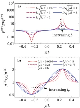
To demonstrate the implications of a pressure which only depends on the local curvature, we establish a connection to the simulations performed in Refs. 21 and 28 and consider the active pressure ˜p(W)(y) on a sinusoidal wall of periodicity L spec-ified by the modulation function M(y) = sin(2πy/L)/2 [the bulk can be found at x < M(y)]. Employing the strategy described above, we define ˜p(W)(y) = p(W)(κ(y)), substituting the local curvature κ(y) = d M ′′(y) (1 + d2M′(y)2)32 = − d 2π2 L2 sin(2πy/L) (1 +d2π2cos2(2πy/L) L2 ) 3 2 (31)
into Eq.(23). InFig. 5, we illustrate the behavior of ˜p(W)(y)/p(W)for different parameters. The overall qualitative picture is in nice agree-ment with the numerical expectation21,28that the pressure becomes extremal at the apices of the modulation function, with its maximum in the negatively curved region. Increasing L at constant persistence length lp[Fig. 5(a)] or, vice versa, decreasing lpat constant L (not
shown), the amplitude decreases. Choosing L/√lp= const, we can
ensure that the maximal and minimal pressure remain independent of the activity [Fig. 5(b)].
FIG. 5. Pressure ˜p(W)(y) of an active ideal gas on a nearly hard sinusoidal wall
of period L parametrized by the coordinate y (see text). The pressure normalized by its bulk value depends explicitly on both L and the persistence length lp. We
compare the data for (a) changing L at constant persistence length lp= 0.6d and
(b) changing lp/d and adapting L according to a fixed ratio L/
√
lpd= 4 so that the
extreme values of the curvature remain constant.
However, there are two observations which highlight some underlying quantitative flaws of the theory. First, the average pres-sure⟨p(W)⟩ = ∫0Ldy ˜p(W)(y)/L is always larger than the bulk value
p(W)for the chosen periodic modulation since it becomes obvious fromFig. 3and also Eq.(23)that p(W)(−κ) − p(W)≥ p(W)− p(W)(κ) for all κ> 0 with an equality only in the planar limit κ → 0. Hence, only for sufficiently large L or small lp,Fig. 5illustrates that the ratio
⟨p(W)⟩/p(W)consistently approaches 1, which is an obvious result in
both limits L→ ∞ of a flat wall and lp → 0 of a passive system.
Second, the theoretical pressure ˜p(W)(nL/2) at the points with zero curvature is always equal to the bulk value p(W), whereas simulations predict a smaller local pressure.21,28This also appears to be the rea-son for the first inconsistency. The expected nonlocal dependence on the wall curvature makes sense when considering the active nature of the particle: it will slide along the boundary until it detaches— either due to reorientation or due to a change in the structure of the wall. For the given wall modulation, the change in the curvature pro-vides a way for particles to escape the flat part of the wall, lowering the density of particles at the wall (and hence the pressure) in the vicinity. Only in the limit of an infinite persistence length, a local dependence on the wall curvature can be expected.25
C. Interactions and wall softness
Our final goal is now to continue the numerical study of inter-acting active and effective systems from Sec.III Awith a focus on
curvature dependence. We know from Sec.IV B 1that a proper comparison of different models is problematic for highly curved boundaries and from Sec.IV B 2that the EPA does not capture a nonlocal dependence on the curvature. Thus, to only judge the qual-ity of the effective pair interaction potential in a curved system, we return to circular walls and restrict ourselves to the initial slope mp, given by Eq.(26). Note that, while we focus in our simulations on the case of a circular cavity of (very large) radius R, the initial slope is expected to be the same for a circular cavity and a circular obsta-cle, and numerical tests for selected points confirm this. For systems with sufficiently low activity (lp≪ R), the first-order result mpshould
still provide a good estimate for the curvature dependence of the wall pressure. In further contrast to the study in Sec.IV B 1, it is necessary for the computer simulations of an interacting system to consider a slightly soft wall. In general, this will be taken into account by choosing the finite value λ = 3000 of the softness parameters in the interaction potentials; compareAppendix B. Also recall that the bulk formula p(B)actcannot be used to study the dependence on the wall
curvature.
1. Active ideal gas at a soft circular wall
As a first step, we need to understand the role of the softness of the wall for an active ideal gas, which is recovered as the low-density limit of an interacting system. The softness parameter λ of the wall potential (compareAppendix B) now provides an additional length scale, and the results do not any more depend only on one univer-sal argument. The theory suggests that the initial slope mpdepends explicitly on both the product of λ with the persistence time τ, as well as, the persistence length lp, even if we divide by lp. Only for
very large values of λτ, all theoretical curves inFig. 6(a)for different persistence lengths lp collapse on the same line, i.e., the persistent
limit is formally equivalent to the hard-wall limit (infinite λ). Note that the limit of τ→ 0 at fixed self-propulsion velocity (as shown in
Fig. 6) does not correspond to the limit of a passive system (where insteadDa= 1 should be kept fixed).
The main point we wish to make here concerns the relation between pressure and surface tension (or adsorption). Explicitly, in generalization of the study from Sec.IV B 1, we find for a soft cavity p(W-)(R−1) Daρ0 = 1 − √π 2 √ Da(1 + 2λτ) √ λ d R, (32) Γ(−)(R−1) ρ0 = √π 2 √ Da(1 + 2λτ) √ λ d− 1 2 Da(1 + 2λτ) λ d2 R , (33) σ(−)(R−1) Daρ0 = √π 2 √ Da(1 + 2λτ) √ λ d− 1 2 Da λ d2 R . (34)
All expressions are still linear in R−1and reduce to Eqs.(23)–(25)
in the hard-wall limit, λ→ ∞, as well as to Eqs.(29)and(30)in the passive limit,Da= 1 and τ = 0. Apparently, the theory provides
the same analytic coefficients for the initial slope mpof the pressure, the planar surface tension σ(0), and the adsorption Γ(0) at a planar wall. Comparing Eq.(33)with Eq.(34), we notice that the deviation from the effective Gibbs adsorption theorem, compare Eq.(14), at the linear order in curvature is by a term which is independent of the wall softness and solely due to activity, i.e., it (necessarily) vanishes
in the passive limit. These theoretical results are again nicely con-firmed by active simulations, which we compare inFigs. 6(b)and
6(c)for a fixed wall potential. Within numerical accuracy, Eq.(28)
holds for any persistence time in all models considered. These obser-vations suggest that the sum rules discussed in Sec.IV B 1are still at work up to the linear order when we allow for a finite wall softness. Also note that mpis again independent of the route to calculate the pressure (p(W)or p(T)).
In the regime where we study the interacting system (λ = 3000 and τ< 0.05), the results of all models deviate noticeably from the hard-wall limit. For both ABPs and AOUPs, there seems to be a (weak) effect of the strength of the wall potential λ (without the factor τ). This is potentially related to the interplay between the effective interaction range of the wall and the persistence length.
FIG. 6. Initial slope mpof the active pressure on a circular wall, as well as
normal-ized adsorption Γ(0) and active surface tension σ(0) on a planar wall. We consider an ideal gas at a soft wall, with the potential specified inAppendix B. Shown are (a) the identical theoretical results (EPA) for different persistence lengths lpas a
function of the product λτ, where λ is the softness parameter and τ is the persis-tence time. Note that in all cases, Eq.(28)is fulfilled. In the hard wall limit, λ→ ∞, all curves approach−√π/2, compare, e.g., Eq.(23). We also compare, as a func-tion of τ, simulafunc-tion results of all three quantities for (b) AOUPs and (c) ABPs to the EPA. Here, we use the softness parameter λ = 3000 and self-propulsion velocity
v0= 24d/τ0.
Up to the offset between the different models already observed for a hard wall, all curves inFigs. 6(b)and6(c)are qualitatively sim-ilar to the theoretical result. However, the slightly different slope of mpin the different models gives rise to a spurious point where the theory and simulations are in perfect agreement. The corre-sponding parameter τ = 0.025 for ABPs appears to be a conve-nient choice to study the influence of interactions although the agreement is rather coincidental. Note, however, that the differ-ences observed for such small τ are insignificant since we normalize here by the persistence length which becomes equally small in this region.
2. Interacting particles at a curved surface
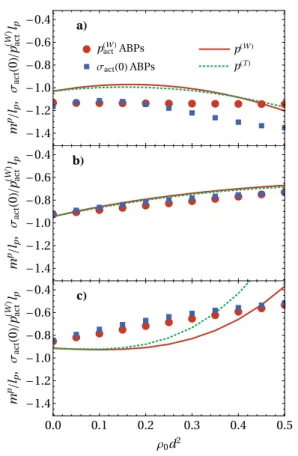
We now compare the curvature dependence in interacting active and effective systems, where we focus our attention on ABPs only. InFig. 7, we show the initial slope mpas a function of the
FIG. 7. Initial slope mp, given by Eq.(26), of the dependence of the active
pres-sure p on the wall curvature R−1in an interacting system of ABPs, as a function of density ρ0. We compare the wall pressure p(W)act, measured directly in an active
system, and the bare and effective wall pressure p(W)and p(T), measured in the
corresponding passive system according to Eqs.(10)and(11), respectively. More-over, we show the normalized active surface tension σact(0) measured for ABPs
at a planar wall. We consider three different persistence times (a) τ = 0.01, (b) τ = 0.025, and (c) τ = 0.05 at fixed self-propulsion speed v0= 24d/τ0and use the
same scale on all axes for a better comparison of the influence of activity on the density dependence. Note that the points corresponding to ABPs are based on fits to the simulation data. The τ-dependent offset at ρ0= 0, described in Sec.IV C 1,
should not be mistaken for an optimal agreement at intermediate activity.
density for different activity parameters, as well as the active sur-face tension at a flat wall σact(0). For ρ0= 0, the result is equal to that
of an ideal-gas for the corresponding parameters, which explains the offset between the curves for ABPs and the EPA. Despite this system-atic deviation, the density dependence of the EPA result p(W)(R−1) shows adequate agreement with the wall pressure of the active sys-tem, demonstrating that the EPA correctly captures the curvature dependence of the wall pressure, as long as the curvature is not too high. In particular, the interplay between interactions, activity and curvature, which we discuss at the end of this section, can be qualitatively reproduced.
At finite densities, the normalized initial slope m/lpexplicitly
depends on both the chosen persistence time and persistence length since there is an additional length scale given by the particle size. Interestingly, the initial slope mpof the curvature dependence for both theoretical pressures p(W)and p(T)is identical within our error bars at low activity even though the predicted pressures are not the same, cf.,Fig. 1. This can be understood from the fact that the curvature-dependence of the wall pressure is mainly caused by the variation in particle density at the wall, i.e., the planar adsorption, and both pressures are based on the same density profile. However, at higher activity (τ = 0.05), we begin to observe deviations between the two.
For the investigated activities, the active surface tension σact(0)
again matches the linear effect of curvature on the pressure mp. The largest deviation is seen at weak activity, where accurate determi-nation of both the surface tension and the slope of the curvature-dependence of the pressure is hard to resolve accurately. Our estima-tion of the statistical errors inherent in our numerical data suggests that within our accuracy, the relation between surface tension and pressure on a curved wall is maintained even for interacting active systems. Note, however, that due to the necessity to fit our data and extrapolate to the limit of large cavities, our statistical errors in the surface tension are rather large, especially for small τ, where the effects we measure are weak. We estimate that error bars in σactare
on the order of 25%, 15%, and 10% for persistence times τ = 0.01, 0.025, and 0.05, respectively.
From our simulations, we observe that for high activity the effect of curvature on the pressure decreases significantly in a dense system, which becomes apparent from the decreasing abso-lute value of the initial slope in Figs. 7(b)and 7(c) for increas-ing density. A possible explanation for this stems from the escape mechanism of a trapped particle. In order for a particle to move away from any wall, it has to rotate its swimming direction away from its normal vector. A negative curvature (cavity) hinders this, as during this process, the particle will slide along the wall toward the point where its swimming direction points toward the wall again. However, if the particle encounters another particle dur-ing this process, this sliddur-ing is inhibited, facilitatdur-ing wall escape. Hence, if the density near the wall is high enough that the parti-cles are likely to collide before they reorient, the effect of curvature is diminished. This is indeed expected to occur at high densities and strong activity. For lower activity, this trend competes with the (passive) surface tension, which tends to increase with num-ber density, so that in the case shown inFig. 7(a)the initial slope remains nearly constant. The theory approximately reflects this behavior.