Node Overlap Removal for 1D Graph Layout

HAL Id: lirmm-01542283

https://hal-lirmm.ccsd.cnrs.fr/lirmm-01542283v2

Submitted on 13 Jul 2017

HAL is a multi-disciplinary open access

archive for the deposit and dissemination of

sci-entific research documents, whether they are

pub-lished or not. The documents may come from

teaching and research institutions in France or

abroad, or from public or private research centers.

L’archive ouverte pluridisciplinaire HAL, est

destinée au dépôt et à la diffusion de documents

scientifiques de niveau recherche, publiés ou non,

émanant des établissements d’enseignement et de

recherche français ou étrangers, des laboratoires

publics ou privés.

Node Overlap Removal for 1D Graph Layout

Samiha Fadloun, Pascal Poncelet, Julien Rabatel, Mathieu Roche, Arnaud

Sallaberry

To cite this version:

Samiha Fadloun, Pascal Poncelet, Julien Rabatel, Mathieu Roche, Arnaud Sallaberry. Node Overlap

Removal for 1D Graph Layout. IV: Information Visualisation, Jul 2017, London, United Kingdom.

pp.224-229, �10.1109/iV.2017.14�. �lirmm-01542283v2�

Node Overlap Removal for 1D Graph Layout

Samiha Fadloun, Pascal Poncelet, Julien Rabatel

Montpellier, France

Email: firstname.lastname@lirmm.fr

Mathieu Roche

Arnaud Sallaberry

Montpellier, France Email: arnaud.sallaberry@lirmm.fr

Abstract—Energy based algorithms are powerful techniques for laying out graphs. They tend to generate aesthetically pleasing graph embeddings, exhibiting symmetries and commu-nity structures. When dealing with large graphs, an important drawback of these algorithms is to produce embeddings where many nodes overlap, leading to cluttering issues. While several approaches have been proposed for node overlap removal on 2D graph layouts, to the best of our knowledge, there is no work dedicated to 1D graph layouts. In this paper, we first define 4 requirements for 1D graph node overlap removal. Then, we propose a O(|V|log(|V|)) time algorithm meeting these requirements. We illustrate our approach with two case studies based on arc diagrams where nodes are positioned by applying a MDS technique to highlight community structures. Finally, we compare our technique with alternatives from 2D graph techniques, and a discussion highlights some properties of the results.

I. INTRODUCTION

1D graph layout is often performed by positioning nodes evenly along an axis and drawing edges as curves above or below the axis. This type of diagram is known as an Arc Diagram [1]. So far, the main concern has been to find an ordering among the nodes that minimizes edge lengths. This problem is called Minimum Linear Arrangement [2], [3].

An alternative to positioning the nodes evenly along an axis is to use Multidimensional Scaling (MDS) [4]. For graph drawing, the input dissimilarity matrix usually corresponds to the path lengths between nodes and the algorithms tend to position the nodes in such a way that the distances in the embedding reflect the path lengths in the graph. The main advantage of this type of techniques is to group the nodes of dense portions of the graph, highlighting path lengths between nodes, symmetries and community structures. Bibliography on MDS for graph drawing includes [5], [6], [7], [8] for 2D embeddings, and [9], [10] for 1D embeddings. When dealing with large graphs, an important drawback of MDS techniques is that it produces embeddings where many nodes overlap, leading to cluttering issues. Several algorithms have been proposed to deal with this issue for 2D graph layout [11], [12], [13], [14], [15], [16], [17]. The purpose of these works is to avoid overlapping and try to preserve the initial configuration of the nodes as much as possible. To our knowledge, no algorithm has been proposed for 1D graph layout exclusively. Our contribution comes in two forms. (1) We give a formal definition of the node overlap problem for 1D layout. It is composed by 4 requirements. While some of them have been addressed by 2D approaches, and could be adapted to 1D, the

4th requirement is new and holds very interesting properties on the layout. (2) We propose a method meeting these require-ments and illustrate the results with two case studies. This case study shows that it is interesting to specifically address the 1D graph layout overlapping problem.

This paper is organized as follows. We first define the 4 requirements for 1D graph node overlap removal in Section II. Then, we propose a O(|V|log(|V|)) time algorithm meeting these requirements in Section III. We illustrate our approach with two case studies in Section IV. We discuss some inter-esting properties held by the 4 requirements in Section V, and we compare our technique with alternatives in Section VI. We conclude in Section VII.

II. PROBLEMSTATEMENT

Let V be a set of nodes {v1, v2, . . . , v|V |} and p a function

V → R+_{∪ {0} denoting the initial 1D layout of the nodes.}

We define an ordering function σ : V → {1, . . . , |V |} w.r.t the initial layout. More formally, for any pair (u, v) ∈ V2

with σ(u) + 1 = σ(v), @w ∈ V |p(u) < p(w) < p(v). If there exists (u, v) ∈ V2 such that p(u) = p(v), we consider an arbitrary strict total order over the nodes V to satisfy the following constraint: ∀(u, v) ∈ V2, u 6= v ⇒ σ(u) 6= σ(v). σ−1 is the inverse function σ−1 : {1, . . . , |V |} → V such that σ−1_{(i) = v ∈ V ⇔ σ(v) = i. A function s : V → R}+ denotes the sizes of the nodes.

We need to find a function f : V → [0, l] that removes overlap between nodes. l is the length of the segment on which we want to position the nodes. This rearrangement allows (i) to improve the visualization of the elements in a 1D graph embedding, and (ii) to preserve the main characteristics of the initial layout (e.g. order and size of nodes). We define a set of requirements for f to preserve the global configuration of the initial layout:

Requirement 1. The final layout should optimally use the length of the segment:

• f (σ−1(1)) = 0 + s(σ−1(1))/2;

• f (σ−1(|V |)) = l − s(σ−1(|V |))/2.

Requirement 2. The final layout should not have nodes overlapping:

Requirement 3. The final layout should preserve the initial ordering. As nodes should not overlap, the requirement can be formalized as:

∀(u, v) ∈ V2, σ(u) < σ(v) ⇒ f (u) < f (v)

Requirement 4. The final layout should preserve the relative distances between consecutive pairs of nodes: ∀((u, v), (u0_{, v}0_{)) ∈ V}2 _{× V}2 _{such that σ(u) + 1 = σ(v)}

and σ(u0) + 1 = σ(v0), p(v) − p(u) ≥ p(v0) − p(u0) ⇒ f (v) −s(v) 2 − f (u) − s(u) 2 ≥ f (v 0_{) −}s(v0) 2 − f (u 0_{) −}s(u0) 2 We assume thatP

v∈V s(v) ≤ l, otherwise, the problem has

no solution because the length of the segment on which the nodes are mapped is not long enough to contain all the nodes without overlapping. In the case whereP

v∈V s(v) = l, nodes

will be positioned evenly and side by side along the segment according to the ordering function σ.

It is essential to notice that Requirement 4 defines the dis-tance between two consecutive nodes u and v as the disdis-tance between their respective borders, while it could be defined as the distance between their centers. The consequences of this choice are further discussed in Section V.

III. OUR PROPOSAL

We propose a function satisfying each of the requirements listed in Section II. To this end, we first define p0as a function scaling the values of p(v), for v ∈ V , into the interval [0, l − P

x∈V s(x)] as follows, with pmin= p(σ−1(1)) and pmax=

p(σ−1(|V |)): p0(v) = p(v) − pmin pmax− pmin × (l − X x∈V s(x))

From an intuitive point of view, this modified positioning function considers only the length of the segment that is still available once all nodes have been placed on the segment without overlapping, i.e., l − P

x∈V s(x). In addition, the

function p0ensures that this available length is used optimally, in the sense of Requirement 1.

Since p(v) − pmin and pmax − pmin are positive, then

p0(v) ≥ p0(u) ⇔ p(v) ≥ p(u). Therefore, p0 conserves the order provided by p. Moreover, ∀(u, v) ∈ V2_{, σ(u) < σ(v) ⇒}

p0(u) ≤ p0(v) and if p(u) = p(v), then p0(u) = p0(v). The proposed node overlap removal function f uses the p0 function and considers the size of each node, so that the position of the center of a node v is given by p0(v) to which is added the radius of v and the size of each node positioned before v. To define formally:

f (v) = p0(v) −s(v) 2 + σ(v) X i=1 s(σ−1(i))

We have already seen that p(u) = p(v) ⇒ p0(u) = p0_(v).

We also mentioned that if p(u) = p(v), we consider an arbitrary strict total order over the nodes V to define σ. For

instance, let’s consider u and v such that p(u) = p(v) and σ(v) = σ(u) + 1. In this case, f (v) = f (u)+s(u)/2+s(v)/2, i.e. nodes are positioned side by side without overlap. Theorem 1. Function f meets the four above-defined require-ments.

Proof. Please see the online report [18] for a complete proof.

Theorem 2. Given an initial 1D embedding of a graph, an overlapping-free layout can be computed in O(|V|log(|V|)) time.

Proof. Given the function p, the order σ is computed in O(|V|log(|V|)) time. The value of f for all nodes is computed in O(|V|), by processing nodes w.r.t. the order σ and storing the cumulative sizes of previously processed nodes in a variable.

IV. CASESTUDIES

A. Les Mis´erables

This first case study is performed on the dataset Les Mis´erables [19]. Each node stands for one character of the Victor Hugo’s novel. An edge connecting a pair of nodes describes that these two characters co-occur in at least one chapter. The size of each node is obtained by summing the number of co-occurrences of the corresponding character. It corresponds to the degree of the node.

Figure 1 shows two distinct 1D representations of this dataset. Figure 1(a) stands for the initial layout, obtained by applying an MDS approach [20]. This layout contains node overlapping. Figure 1(b) shows the same data without node overlapping, obtained by applying our method for the same segment length. From this global views, one can already notice some additional information due to the proposed method. For instance, the left-most part of the initial layout seems to be composed of only one node from which one edge leaves and is then split into 4 distinct edges linking this element to the 4 closest nodes. The second layout, obtained by removing node overlapping, shows that the left-most node of the initial layout is in fact composed of multiple small nodes, and allows the user to identify how each individual node (i.e., character) is connected to other elements.

(a)

(b)

Fig. 1. Two distinct 1D layouts of Les Mis´erables dataset, the above one (a) is an initial layout containing some node overlap, while the bottom one (b) has been constructed by our proposed node overlap removing method.

For the sake of readability, Figure 2 proposes a closer look into a subpart of the previous visualizations. Figure 2(a) and Figure 2(b) correspond to the same subset of nodes, respectively with the initial layout and the proposed one (edges have been removed to allow a better focus on node placement).

Fig. 2. Subpart of Les Mis´erables dataset from the initial layout (a) and our proposed method (b). The correspondences between the main clusters in both layouts are highlighted in light gray.

One first observation focuses on the importance of node overlapping removal. In Figure 2(a), nodes are often overlap-ping to the extent where the visualization allows one to see some clusters in the data, but prevents any analysis at the node (i.e., character) level. From this point of view, the proposed method plays its role as expected, by showing next to each other all the nodes that were initially part of the same set of overlapping nodes, hence providing a better readability of the data at the finest granularity. As an example, one may consider the right-most cluster from the top visualization, that is composed of many more nodes than one may expect by simply considering the initial layout.

In addition, the proposed layout also has the advantage of showing that some nodes such as Favourite, that initially seemed very close to the other nodes, clearly appears distinctly from the rest.

We are convinced that the proposed layout gives a more natural way of analysing the distances between consecutive pairs of nodes. As an example, one may more easily observe in the proposed layout that the distance between characters Valjean and Marguerite (represented as the empty space be-tween the two nodes) is approximately 1/3 of the distance between Marguerite and Madame de R. This observation is more difficult to obtain from the initial layout, in particular when nodes have different sizes, as it requires the user to consider the distance between node’s centers (see section V for more details about the benefits of requirement 4).

We additionnally notice that nodes that were initially ap-pearing alone, such as Marguerite, also appear alone in the final layout.

B. PacificVis co-authorship network

The second case study is performed on a PacificVis co-authorship network extracted from DBLP. Each node of the graph stands for an author having published at least 3 papers in the Asia Pacific Symposium on Information Visualization (PacificVis) between 2008 and 2016. There is an edge between two nodes if the corresponding authors have published at least one paper together. We also extracted, for each author,

a vector containing the number of papers they have published in PacificVis by year. The size of each node is obtained by summing the values of an author’s vector. It corresponds to the total number of papers published by the author at PacificVis during this period.

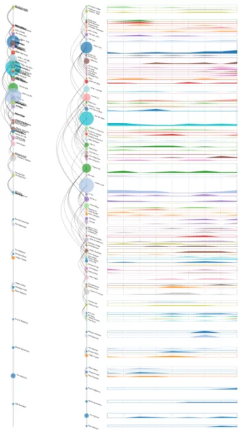
Fig. 3. PacificVis co-authorship network extracted from DBLP, with overlaps (left), no overlap (center) and corresponding silhouette graphs (right).

Rufiange and McGuffin [21] propose a taxonomy of 5 strategies for visualizing dynamic graphs (see Figure 2 of their article). It is important to notice that the concept of dynamic graph such as developed in the article covers both (i) topo-logical changes and (ii) numerical attribute changes. The 4th strategy consists in visualizing the time axis perpendicularly to an arc diagram. In their example, the time axis represents the evolution of a numerical attribute, and authors cite 4 papers exclusively dealing with graphs having topological changes.

In this section, we focus on the 4th strategy when dealing with a numerical attribute changes, as in the example of Rufiange and McGuffin’s paper. The co-authorship network is represented as a vertical diagram (see Figure 3). Nodes are

positioned by applying an MDS approach [20] followed by our method to remove node overlapping. The vector containing the number of papers published each year by an author is repre-sented by an horizontal silhouette graph [22] beside each node. The height of the silhouette graph bounding box represents the total number of papers published by the corresponding author and is is equivalent to the node size. This uniform vertical scale for silhouette graphs, in addition to the vertical alignment of years, ensures that publication numbers are easy to compare from one author to another. Vertical grey lines represent years. Each connected component of the network has been processed separately, and the corresponding results have been placed vertically on the same layout, in an arbitrary order. Colors are provided by the default configuration of the D3 library [23].

Figure 3 shows that the network consists of 8 connected components. The first one (from the top) contains a very large fraction of the node set. It is followed by one 2-elements connected component, two 3-elements connected components and 4 singletons.

Fig. 4. Subpart of the PacificVis co-authorship network.

The graph layout (MDS + node overlap removal method) naturally allows to highlight the relative importance of nodes, which is here related to the number of publications during the 2008-2016 period, as well as some communities within the data with a clear readability at the node level. In addition, the right part of the visualization allows one to easily obtain more information about each node w.r.t. the time dimension. In the following, we discuss the advantages of the proposed 1D graph layout in such a setting.

(a) (b) (c) (d)

Fig. 5. Various authors from the PacificVis co-authorship network exhibiting different publication profiles over the years.

Figure 4 focuses on a subpart of the co-authorship network, in which three subsets of authors (denoted as S1, S2 and S3) interact with each other in interesting ways. The distance between the elements of each subset shows that they are part of distinct small communities in the network. It is interesting to notice that S2 plays a role of pivot regarding communities

S1 and S3. Indeed, authors in S1 and S3 have no direct connections (i.e., co-authored publications) but almost all of them are connected to one or two authors of S2. It is also interesting to observe that authors of a same community often share a similar publication silhouette graph.

One relevant aspect of this visualization strategy is that it also allows a very readable analysis of publication distribution profiles of authors, as well as an easy way to compare them. Figure 5 provides a selection of authors with close total numbers of publications (i.e., node sizes), whose respective publication silhouette graphs however expose different no-ticeable profiles. As an example, Figure 5(a) corresponds to an author whose publication record in PacificVis exhibits a particular regularity during most of the considered period. This publication distribution profile contrasts with the more sporadic one provided by Figure 5(b), where the total amount of publications is shared among two conference editions. The third author from Figure 5(c), shows a progression profile, where the publication count started and grew during the last two years. Figure 5(d) shows a particular case where all the publications occurred during the same year. This case is easily noticeable as the silhouette graph value reaches the border of the bounding box.

From a more general point of view, it can be noticed that the obtained visualization, by vertically aligning silhouette graphs, makes it considerably easy to compare publication profiles over time, as well as to compare numbers of publications for a given year. This aid in comparing elements of the network would be much more difficult to obtain with the other 4 visual representation strategies proposed by Rufiange and McGuffin [21], which are all based on a 2D graph layout. It is interesting to notice that none of them allows such an ease of analysis when the user needs to visually compare the count of publications over the years. This case study shows how a 1D graph layout can be a relevant alternative to 2D graph layout, or even a superior one for some tasks, for instance comparing nodes with associated timeseries data [24].

This advantage is mainly due to the fact that using a 1D graph layout for positioning the nodes allows the visual rep-resentation to fully exploit an additional available dimension for representing the dynamic feature of the graph (i.e., the publication distribution over time in our use case). Usually, the use of a 1D graph layout rather than a 2D one implies an important cost at the data structure visualization level, due to: (1) the lack of readability, this is for instance the case when using an MDS approach for placing the nodes, resulting in node overlapping ; (2) the lack of information, this is the case when exploiting a Minimum Linear Arrangement approach that results in nodes being placed uniformly along the segment, hence providing no information about the similarity between nodes. This case study shows that the cost of using a 1D graph layout rather than a 2D one is reduced when exploiting the proposed approach, as it both removes node overlapping and conserves the properties of the initial data in terms of node similarity.

V. DISCUSSION

A. Node Proximity.

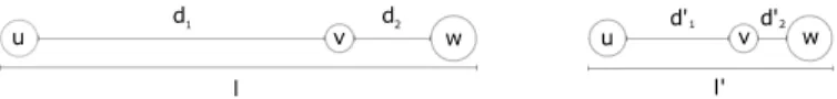
Existing techniques for removing node overlapping in 2D graphs (e.g., [14], [16]) move nodes from the initial embedding until no more overlapping exist in the layout (see Section VI for more details). As a result, distances between pairs of nodes in the final layout depend on how nodes were overlapping in the initial layout and the Requirement 4 is not always met. It is different with our method. Figure 6 shows an example of a graph composed of three nodes u, v and w, with two layouts obtained by decreasing the length of the segment l to l0. In this case, the distance between consecutive nodes (i.e., the length between their closest borders) linearly decreases while the segment length decreases. In other terms, the distance ratios remain identical: d1/d2= d01/d02. While 2D approaches have

the advantage of highlighting clusters, they do not allow the user to precisely assess the real similarity between two nodes. On the contrary, the method that we propose always retains the exact relative distances w.r.t. the initial layout.

Fig. 6. Two layouts obtained by decreasing the length of the segment l to l0_.

B. Distance Perception.

The initial layout, referred as function p in Section II, in addition to allowing node overlapping, can also have the draw-back of leading users to wrongly interpret distances between nodes. Let us consider the example provided in Figure 7. Three nodes u, v and w are thereby presented following two distinct 1D layouts: the initial one provided by function p and the one proposed in this paper.

In the initial layout, one may notice that one node being included in another makes these nodes perceived as similar whereas they are not. It is noticeably the case with nodes u and v that seem to appear closer than v and w. However, if looking more carefully at the distances between the center of nodes without considering their size, one may easily observe that this is a perception error: v and w are actually at the same distance than u and v. This well-known perception bias is directly related to the Gestalt law of continuity.

Our approach aims at providing a simple and effective so-lution to this problem, by defining a layout where the distance between two nodes is mapped onto the distance between their closest borders. Our layout illustrates this claim as nodes v and w appear to be as close as u and v, which correctly reflects the data. This principle is at the core of the proposed layout and provides the end-user with a visualization that reflects the way his/her perception works. Requirement 4 hence seems to allow a quicker and more relevant understanding of the data, which can help identifying underlying clusters.

Fig. 7. Initial layout (left) and our proposed layout (right).

VI. ALTERNATIVE TECHNIQUES

Many approaches have been proposed to remove node overlapping in 2D graph embeddings. Most of them [11], [12], [13], [25], [14], [15], [17] can be applied to 1D embeddings. They all fall into two main categories: Force Scan Algorithms (FSA) and Constraint Optimization based Approaches (COA). While their 1D versions meet the 2nd requirement (no over-lapping), it is not obvious that they meet the other ones. In this section, we give a brief description of these algorithms and their requirement satisfaction and time complexity.

FSA, introduced by Misue et al. in [11], is a major approach of the first category. The idea is to apply a force function f on overlapping nodes: if a node u overlaps a node v, then f (u, v) pushes v away from u. Authors propose a “pushing” force model and an algorithm to apply this model for removing node overlapping (Push Force Scan Algorithm). Forces for all nodes are first applied horizontally, then vertically, so the algorithm can be applied on a 1D embedding. Authors also propose a second force model allowing “pulling” forces as well as “pushing” forces: (Push-Pull Force Scan Algorithm). The embedding is thus more compact. In [12], Hayashi et al. prove that finding the minimum area layout of the nodes that avoids intersections of the shapes and preserves the orthogonal order is NP-complete. In addition, they propose a heuristic algorithm based on the same idea as FSA that positions the nodes into a smaller area. Another work of Li et al. [25] also presents two other variants of FSA giving a smaller area. Huang et al. introduce the Force-Transfer Algorithm (FTA) in [15]. The algorithm starts with a seed node and finds the cluster of overlapping nodes containing the seed node among one dimension (horizontal or vertical). Then, a force model is applied to remove overlaps in the cluster. Some nodes might newly overlap with nodes outside the cluster, so a new cluster is formed dynamically. The process ends when each nodes’ cluster is empty. The same process is then applied to the other dimension. Abe et al. refine the algorithm in [17]. The output of FTA is more compact than the one provided by FSA. FSA and FTA algorithms preserve orthogonal ordering, except one presented in [25]. Thus, the 1D version meets the 3rd requirement. The area devoted to the final embedding is not bounded so the algorithm does not meet the 1st requirement. As the sizes of the nodes are not considered, the 4th requirement is not met either. They have a complexity of O(|V |2), for both horizontal and vertical scans. Applying them in one dimension gives the same complexity.

COA focuses on minimizing an objective function while preserving a set of constraints. The objective function rep-resents node movements. The constraints ensure that nodes

don’t overlap each other. Removing the node overlaps is thus addressed as a constraint optimization problem. In [14], Dwyer et al. propose an algorithm for finding separation constraints between nodes, and another one to solve the corresponding optimization problem. This algorithm can be applied to 1D graph layout. It doesn’t meet requirements 1 and 4. Even if the objective function ensures small changes of nodes’ positions, it doesn’t guarantee that the initial orthogonal ordering is preserved (requirement 3 in 1D layout). Another work proposed by Marriott et al. [13] describes four different COA approaches. None of them meets requirements 1, 3 and 4. COA approaches require to first find the constraints and then remove overlaps. In [14], the complexity for finding the sep-aration constraint is O(|V |log|V |). The constraint satisfying algorithm runs in O((|V | · |C|)log|C|) where C is the set of constraints (the number of these contraints is O(|V |)) [26]. In [13], the complexity of finding an overlapping-free solution is O(|V |2_{· log(|V |)) for the first approach based on uniform}

scaling. Other approaches described in the paper are more time consuming.

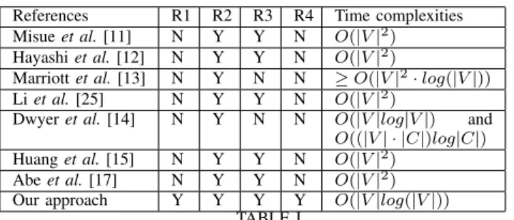
Table I sums up the properties of the different alternatives as well as their time complexities. One can observe that our algorithm is the fastest and the only one to meet the 4 requirements. This is due to the fact that it is the only one exclusively devoted to solve the 1D version of the problem. We did not include the approach proposed by [16] because its adaptation to the 1D case is not trivial.

References R1 R2 R3 R4 Time complexities Misue et al. [11] N Y Y N O(|V |2₎

Hayashi et al. [12] N Y Y N O(|V |2₎

Marriott et al. [13] N Y N N ≥ O(|V |2_{· log(|V |))}

Li et al. [25] N Y Y N O(|V |2₎

Dwyer et al. [14] N Y N N O(|V |log|V |) and O((|V | · |C|)log|C|) Huang et al. [15] N Y Y N O(|V |2₎

Abe et al. [17] N Y Y N O(|V |2₎

Our approach Y Y Y Y O(|V |log(|V |)) TABLE I

COMPARISON OF THE DIFFERENT APPROACHES FOR REMOVING NODE OVERLAPS IN1DLAYOUT: “N”STANDS FOR“NO”, “Y”FOR“YES”.

VII. CONCLUSION

In this paper, we have first proposed 4 requirements to re-move overlapping of 1D graph layout. We then have proposed a O(|V|log(|V|)) time algorithm meeting these requirements and illustrated it with two case studies based on arc diagrams where nodes are positioned by applying a MDS technique to highlight community structures. A discussion highlights nice properties of the requirements, and shows that the 4th one is essential to reflect correctly the data structures. Finally, we have also shown that current state-of-the-art alternatives do not meet the 4 requirements. As a future work, we will study the possibility to extend our approach to 2D graph layouts.

ACKNOWLEDGMENT

This work has been carried out thanks to the support of the LabEx NUMEV project (no ANR-10-LABX-20) funded by

the “Investissements d’Avenir” French Government program, managed by the French National Research Agency (ANR).

REFERENCES

[1] M. Wattenberg, “Arc diagrams: visualizing structure in strings,” in Proc. InfoVis, 2002, pp. 110–116.

[2] J. Petit, “Experiments on the minimum linear arrangement problem,” ACM Journal of Experimental Algorithmics, vol. 8, 2003.

[3] Y. Koren and D. Harel, “A multi-scale algorithm for the linear arrange-ment problem,” in Proc. WG, ser. LNCS, vol. 2573. Springer, 2002, pp. 296–309.

[4] I. Brog and P. J. F. Groenen, Modern multidimensional scaling : Theory and applications. Springer-Verlag, 1997.

[5] T. Kamada and S. Kawai, “An algorithm for drawing general undirected graphs,” Information Processing Letters, vol. 31, pp. 7–15, 1989. [6] E. R. Gansner, Y. Koren, and S. North, “Graph drawing by stress

majorization,” in Proc. Graph Drawing, ser. LNCS, vol. 3383. Springer, 2004, pp. 285–295.

[7] U. Brandes and C. Pich, “An experimental study on distance-based graph drawing,” in Proc. Graph Drawing, ser. LNCS, vol. 5417. Springer, 2009, pp. 218–229.

[8] C. Pich, “Applications of multidimensional scaling to graph drawing,” Ph.D. dissertation, Universitt Konstanz, 2009.

[9] Y. Koren and D. Harel, “Axis-by-axis stress minimization,” in Proc. Graph Drawing, ser. LNCS, vol. 2912. Springer Berlin Heidelberg, 2004, pp. 450–459.

[10] ——, “One-dimensional layout optimization, with applications to graph drawing by axis separation,” Computational Geometry, vol. 32, no. 2, pp. 115–138, 2005.

[11] K. Misue, P. Eades, W. Lai, and K. Sugiyama, “Layout adjustment and the mental map,” Journal of Visual Languages and Computing, vol. 6, no. 2, pp. 183–210, 1995.

[12] K. Hayashi, M. Inoue, T. Masuzawa, and H. Fujiwara, “A layout adjustment problem for disjoint rectangles preserving orthogonal order,” Systems and Computers in Japan, vol. 33, no. 2, pp. 31–42, 2002. [13] K. Marriott, P. J. Stuckey, V. Tam, and W. He, “Removing node

over-lapping in graph layout using constrained optimization,” Constraints, vol. 8, no. 2, pp. 143–171, 2003.

[14] T. Dwyer, K. Marriott, and P. J. Stuckey, “Fast node overlap removal,” in Proc. Graph Drawing, ser. LNCS, vol. 3843. Springer Berlin Heidelberg, 2006, pp. 153–164.

[15] X. Huang, W. Lai, A. S. M. Sajeev, and J. Gao, “A new algorithm for removing node overlapping in graph visualization,” Information Sciences, vol. 177, no. 14, pp. 2821–2844, 2007.

[16] E. R. Gansner and Y. Hu, “Efficient node overlap removal using a proximity stress model,” in Proc. Graph Drawing, ser. LNCS, vol. 5417. Springer Berlin Heidelberg, 2008, pp. 206–217.

[17] N. Abe, H. Oh, and K. Inoue, “Algorithms for removing node overlaps with some basis nodes,” in Proc. SNPD, ser. Studies in Computational Intelligence, vol. 612. Springer, 2015, pp. 93–102.

[18] S. Fadloun, P. Poncelet, J. Rabatel, M. Roche, and A. Sallaberry, “Node overlap removal for 1d graph layout: Proof of theorem 1,” LIRMM -University of Montpellier, Tech. Rep. lirmm-01521385, 2017. [19] D. E. Knuth, The Stanford GraphBase: a platform for combinatorial

computing. Addison-Wesley Reading, 1993, vol. 37.

[20] J. De Leeuw and P. Mair, “Multidimensional scaling using majorization: Smacof in r,” Department of Statistics, UCLA, 2011.

[21] S. Rufiange and M. J. McGuffin, “Diffani: Visualizing dynamic graphs with a hybrid of difference maps and animation,” IEEE TVCG, vol. 19, no. 12, pp. 2556–2565, 2013.

[22] R. L. Harris, Information Graphics: A Comprehensive Inllustrated Reference. Oxford University Press, New York, USA, 1999. [23] M. Bostock, V. Ogievetsky, and J. Heer, “D3 _{data-driven documents,”}

IEEE TVCG, vol. 17, no. 12, pp. 2301–2309, 2011.

[24] P. Saraiya, P. Lee, and C. North, “Visualization of graphs with associated timeseries data,” in Proc. InfoVis), 2005, pp. 225–232.

[25] W. Li, P. Eades, and N. S. Nikolov, “Using spring algorithms to remove node overlapping,” in Proc. APVIS, 2005, pp. 131–140.

[26] T. Dwyer, K. Marriott, and P. J. Stuckey, “Fast node overlap removal -correction,” in Proc. Graph Drawing, ser. LNCS, vol. 4372. Springer Berlin Heidelberg, 2007, pp. 446–447.