Air/gas system dynamics and implosion control of fossil fuel power plants

(1)

AIR/GAS SYSTEM

DYNAMICS AND

IMPLOSION CONTROL

OF FOSSIL FUEL POWER

PLANTS

by Shang Zhi Wu

M.S., Massachusetts Institute of Technology, 1981 M.S. in Management of Technology, M.I.T., 1984

SUBMITTED TO THE DEPARTMENT OF MECHANICAL ENGINEERING IN PARTIAL FULFILLMENT OF THE REQUIREMENTS FOR

THE DEGREE OF DOCTOR OF PHILOSOPHY

at the

MASSACHUSETTS INSTITUTE OF TECHNOLOGY Copyright ( 1984 Massc et tsnstitute of Technology

Signature of Author

Department of Mechanical Engineering October 19, 1984 Certified by David N. Wormley Thesis Supervisor Accepted by Ain Sonin

SOF TECHNOLOGYTTE Chairman, Department Committee

MAR 2

21985

ARCHIVES LIBRARIE3

(2)

AIR/GAS SYSTEM DYNAMICS AND IMPLOSION CONTROL OF FOSSIL FUEL POWER PLANTS

by Shang Zhi Wu

Submitted to the Department of Mechanical Engineering on October 19, 1984 in partial fulfillment of the requirements for the degree of DOCTOR OF PHILOSOPHY.

Abstract

A computer-based mathematical model for analyzing power plant air/gas system transient dynamics has been developed. The model is formulated by representing power plant air/gas system components as a set of generic elements. This set of generic elements can be connected by generalized junction structures to represent a variety of plant configurations. The response of pressure, flow, temperature and heat transfer rate at any point in air/gas systems subjected to a wide range of fluid, mechanical and thermal disturbances can be determined by computer simulations. Such a formulation and simulation of air/gas system is particularly useful for studies of air/gas pressure dynamics coupled with thermal transients in the same time frame, such as boiler furnace implosions.

To validate the mathematical model and illustrate the use of the computer code, basic plant models for a coal-fired plant and an oil-fired plant have been developed. System responses to main fuel trips are simulated for both plants. The simulation predictions of furnace pressure excursions are in close agressment with the experimental data from field test results.

The computer simulation of the coal-fired plant has been used to evaluate various control systems for furnace and stack implosion protection. The simulation resilts have shown that a well designed draft control system can limit furLace pressure excursions to an acceptable level. The limitations of present control systems are the actuator speed and possible negative pressure

(3)

excursions in the stack during control actions. A preliminary study indicates that discharging steam into the furnace after fuel trip implosion condition may be an effective alternative solution, and the implementation of such a scheme merits further investigation.

Thesis Supervisor: Title:

David N. Wormley

(4)

Acknowledgments

I am very fortunate to have had Professor David N. Wormley supervise both my master's and doctor's thesis. His insight, experience and careful guidance have made our association extremely rewarding for me. I also wish to thank Professors Peter Griffith, Henry M. Paynter and Derek Rowell for serving on my thesis committee. I am grateful for their valuable suggestions, criticism and encouragement.

Special thanks go to James Roseborough, Bruce Eason and John Samon for their technical assistance and helpful discussions, and to Leslie Regan for her help during my five years schooling at M.I.T.

I wish to extend my gratitute to my wife Xiao-xing and my parents for their love and support.

My education at M.I.T. is supported by a scholarship from Chinese Ministry of Educatoin and a research grant from Electric Power Research

(5)

List of Figures

Figure 1-1: Furnace Implosion after a Main Fuel Trip

Figure 2-1: A Typical Power Plant Air/Gas System Configuration

Figure 2-2: Plenum Volume Element

Figure 2-3: Perfect Stirred Reactor (PSR) Model for Combustion Furnace

Figure 2-4: Rosin-Fehling I.T. Diagram Ref. [58]

Figure 2-5: Reaction Rate As A Function Of Temperature

Figure 2-6: Transmission Line Element Representation

Figure 2-7: Centrifugal Fan Symbolkic Representation

Figure 2-8: Typical Centrifugal Fan Characteristics

Figure 2-9: Axial Fan Symbolic Representation

Figure 2-10: Typical Axial Fan Characteristics

Figure 2-11: Symbolic Representation Of Resistance Element

Figure 2-12: Symbolic Representation Of Mechanical Damper

Figure 2-13: Heat Transfer Element

Figure 2-14: Solid Thermal Element

Figure 2-15: Symbolic Representation of Heat Exchanger

Figure 2-16: Heat Exchanger Element Model

Figure 3-1: Typical Decay Of Tracer After Cutoff Injection Ref [48]

Figure 3-2: Bragg's Idealized Combustion Chamber Illustrating The Bragg Criterion, 1 a PST; 2 a Plug-flow Region Ref.-13]

Figure 3-3: PSR Versus Plug-flow Model

Figure 3-4: Step Response Of N - PSR Models

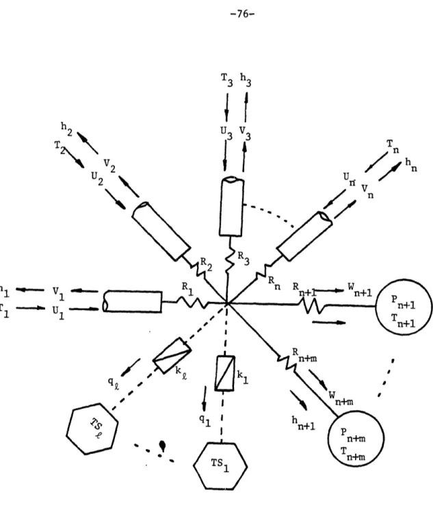
Figure 3-5: General Junction

Figure 3-6: General Junction with Heat Transfer

Figure 3-7: Fan Junction Configurations

Figure 3-8: Axial Fan Junction

Figure 3-9: Axial Fan Junction Bond Graph Representation

Figure 3-10: Heat Exchanger Junction Configurations

Figure 3-11: Typical Heat Absorption Distribution

Figure 3-12: Steady State Furnace Energy Balance Model

Figure 4-1: The Detroit Edison St. Clair Unit 3

Figure 4-2: Mathematical Model for St. Clair Unit 3

Figure 4-3: Mathematical Model for Greenwood Unit 1

Figure 5-1: The General Simulation Causality

Figure 5-2: Computer Simulation Program Flow

Figure 5-3: Computer Model Organization

Figure 6-1: Instrumentation Locations at St. Clair Unit 3 Ref. [14]

Figure 6-2: Pressures Throughout the Unit Ref. [14]

Figure 6-3: Flame Luminosity and Furnace Pressure vs. Time

Ref. [30]

Figure 6-4: Pressure Comparison at Radiant Furnace

Figure 6-5: Pressure Comparison at Convective Furnace

Figure 6-6: Pressure Comparison at Precipitator

19 30 35 35 41 41 46 48 48 51 51 54 54 57 57 60 60 64 64 66 66 68 76 80 83 83 85 89 89 95 96 103 108 112 113 117 119 119 124 124 125

(9)

Figure 6-7: Figure 6-8: Figure 6-9: Figure 6-10: Figure 6-11: Figure 6-12: Figure 6-13: Figure 6-14: Figure 6-15: Load) Figure 7-1: Figure 7-2: Figure 7-3: Figure 7-4: Figure 7-5: Figure 7-6: Figure 8-1: Figure 8-2: Figure 8-3: Figure 8-4: Figure 8-5: Figure 8-6: Figure 8-7: Figure 8-8: Figure 8-9: Figure 8-10: Figure 8-11: Figure 8-12: Figure 8-13: Figure 8-14: Figure 8-15: Figure 8-16: Figure 8-17: Figure A-i: Figure B-1: Ref. [8] Figure B-2: Figure B-3: Ref. 8] Figure B-4: Ref. [8] Figure B-5: Figure B-6: Figure B-7: Figure C-l: Figure C-2:

Flame Luminosity vs. Combustion Energy Generated Temperature in Radiant Furnace

Fuel Concentration in Radiant Furnace

Measurement Location on Greenwood Unit 1 Pressure Comparison at Transducer Location Pressure vs. Time After MFT (100% Load)

Axial ID Fan Operating Locus in Implosion Transient Temperature After MFT (100% Load)

Combustion Energy Generated After MFT (100% Non-Linear Simple Model

Linearized Simple Model

Model Comparison by St. Clair Unit 3 Slow fan Control Action Case

Fast Fan Control Action Case

Model Parameter Sensitivity Simulation

FD Fan Characteristics with/without Duct Holes ID Fan Limiting Control Scheme

General Control Scheme

Feedfoward Controiler Generating Function Flow Reduction Under IGV Control

The ID Fan Bypass Control System Ref. [35] Bypass Control System Model

Steam Discharge Implosion Control Scheme Effect of IGV Control on Both Fans

Limits of Fan IGV Controls

Pressure Drop in Stack under IGV Controls Effect of the ID Fan Bypass Control

Pressure Drop in Stack under Bypass Controls Effect of Both Bypass and IGV Controls

Stack Pressure under Both Bypass and IGV Controls Comparison of Different Draft Control Systems

Steam Discharge For Furnace Implosion Control Fluid Transmission Line Sketch

Critical Temperatures in ASTM Standards D 1857 Typical Coal-Ash Deposit Structure Ref. [81

Softening Temperature of Coal-Ash Free of Iron Oxide Lowering of Softening Temperature from Iron Oxide Coal-Ash Deposit Heat Transfer Model Ref. [81

Thermal Conductivity of Coal-Ash Deposits Ref. [8] Surface Emissivity of Coal-Ash Deposits Ref. [8]

Control Element Representations

The Sensor And Driver Representations

125 126 126 130 130 131 131 132 132 135 135 139 142 143 144 148 148 150 153 153 155 155 158 160 161 162 165 166 167 168 169 170 176 188 188 189 189 191 191 194 196 197

(10)

List of Tables

Table 4-I: Table 4-: Table 6-I: Table 6-II: Table B-I: Table B-II: Ref. [8]

St. Clair Unit 3 Plant Parameters

Estimated Greenwood Unit 1 Plant Parameters Pressure Data at St. Clair Unit 3 Ref. [14

Steady State Gas Condition at Greenwood Unit 1 Density of Various Coal-Ash Deposits Ref. 8]

Emissivities and Absorptivities of Coal-Ash Deposit 100 104 118 129 193 193

(11)

NOMENCLATURE

a - ash deposit absorptivity A - duct cross section area, ft2

Aa - cross section area of axial fan chamber, ft2

Ah - heat transfer area, ft2

Ai - heat transfer area of frnace compartment i. ft2

Ar - flow resistance geometry coefficient A_s - steam discharge valve area, ft2 B - fuel activation energy

C - fuel concentration. lbm/ft2

c - specific heat for solid, Btu/lbm F

cc - heat exchanger cold side fluid specific heat. Btu/lbm F ch - heat exchanger hot side fluid

specific heat. Btu/lbm F CO - speed of sound in fluid, ft/sec

Cox - oxygen concentration, lbm/ft3

Cp - gas specific heat at constant pressure, Btu/lbm F

Cv - gas specific heat at constant volume.

(12)

Cst - specific heat for steam, Btu/lbm F C - specific heat for water, Btu/lbm F d - fan impeller diameter, ft

Do - diffusion coefficient

Ec - combustion energy generated. Btu/sec E, - energy needed to evaporate fuel moisture,

Btu/sec

E_v - rate of energy release. Btu/sec.ft3

f - fuid friction coefficient

G - control gain

h_i - energy flow rate at the ith branch of general junction, Btu/sec

hfg - latent heat value for water, Btu/lbm hJ- net energy flow into junction. But/sec HT - ash hemispherical temperature, F

Hv - fuel heat value, Btu/lbm

I - flow inertance of axial fan element, 1/ft k - thermal conductivity, Btu/ft2,hr.F/ft K - combustion rate constant

k1 - conductivity of primary layer. Btu/hr ft F k2 - conductivity of secondary layer.Btu/hr ft F

kc - reaction collison frequency constant

(13)

1 - heat transfer material thickness, in L - length of transmission line, ft

11 - thickness of primary ash deposit layer, in 12 - thickness of secondary ash deposit layer, in La - length of axial fan chamber, ft

If - mass transfer film thickness, in M - gas mass. bm

Ms - solid mass, lbm

P - pressure (inches of H20 or lbf/ft2)

PJ - pressure at general junction. inches of H₂0

PD - transmission line downsteam pressure, inches of H₂0 PU - transmission line upsteam pressure, inches of H20 APf - pressure drop acoss fans, inches of H₂0

Q - heat transfer, Btu/sec

Qf - volume flow rate. ft3/sec

q - heat transfer rate. Btu/sec. ft2

qi - average heat transfer rate in compartment i, Btu/sec, ft2

r - critical pressure ratio

R - ideal gas constant (=53.3 lbf-ft/lbm R) R_i - flow resistance at ith branch of general

(14)

Rt - combustion rate, lbm/sec.ft3

rc - chemical reaction controlling rate. 1/sec

rm - mass transfer controlling rate. 1/sec S - laplace operator

t - time, sec

T - temperature, °R

TD - wave propagation delay time, sec T_s - ash deposit surface temperature, OR Tis - initial slag temperature, °F

Ttb - water tube temperature. °R Tst - saturated steam temperature, °R Tf - initial fuel temperature. °R

T - junction temperature, OR

TCv - critical temperature for ash, °F

u - fan impeller tip speed, ft/sec

U - internal energy. Btu

Ui - reflected wave variable of ith transmission line at junction, inches of H20

U - convection film conductivity, Btu/hr R ft2 UD - transmission line downstream right wave

inches of H₂0

UU - transmission line upstream right wave inches of H20

(15)

v - flow velocity, ft/sec

V - volume. ft3

VD - transmission line downstream left wave inches of H20

VU - transission line upstream left wave inches of H₂0

W - gas mass flow rate. lbm /sec

WC - heat exchanger cold side flow rate, lbm/sec Wh - heat exchanger hot side flow rate, lbm/sec WJ - net mass flow into junction, lbm/sec

W_i - incoming mass flow, lbm/sec W_O - outgoing mass flow. lbm/sec

WU - transmission line upstream flow

WD - transmission line down stream flow

Wf - fuel flow rate. lbm/sec

Wfs - initial fuel flow rate, lbm/sec

W_s - steam flow rate. lbm/sec

x - distance long transmission line. ft

Zc - transmission line characteristic impedance (sec inches of H20/lbm)

a - fan imlet guide vane or blade angle, degrees aq - quadratic resistance coefficient.

inches of H₂0/(lbm/sec)2 a_d - damper angle, degrees

(16)

- fluid bulk modulus

6f - fraction of ash in fuel

p - fluid density. lbm/ft3 X - fuel moisture fraction

e - ash deposit emissivity

Ef - flame emissivity

a- Stefan - Boltzmann constant for radiation

- fan flow coefficient

T - fan pressure coefficient - slag viscosity, poise

(17)

Chapter 1 INTRODUCTION

1.1 Background

Several dynamic problems are associated with the combustion air, flue and gas recirculation systems of fossil fuel electric power plants. These problems may be broadly classified as (1) steady state pulsation problems resulting in noise or duct and equipment vibration, and (2) transient and control problems leading to a possible implosion condition or instability.

Pulsation problems may generate sufficient noise to represent a health problem, sufficient vibration to result in structural damage or in the case of large amplitude low frequency pressure surging, sufficient pressure variation to cause equipment to trip or fail.

The transient control problem leading to a possible implosion is usually caused by a fuel trip or misoperation of the forced draft or induced draft fans in which the general fan-duct-furnace response leads to an excessively low furnace pressure. In an extreme transient response, the air/gas system may sustain structual damage.

A principal cause of a potential implosion results from a flameout after a main fuel trip (MFT). The basic physical factors resulting in a drop in pressure after a MFT are illustrated in Figure 1-1. Following a MFT, the temperature in the radiant furnace typically decreases from 2500 F to approximately 1000 F in a matter of a few seconds following the cutoff of

(18)

fuel. Since the airflow can not change instantaneously and increase the gas density in the furnace, the furnace pressure drops approximately as described by the ideal gas law. This drop in pressure may be large enough to cause structural damage.

Other potential causes of substantial negative pressure excursions include control system failures and incorrect fan operating procedures. For example, if an FD fan damper is suddenly closed while the ID fan is operating, a drop in furnace pressure occurs as a result of continuous ID fan suction of furnace gas. On the other hand, the negative pressure excursion may occur in the stack if the ID fan damper is suddenly closed.

A number of implosion incidents have been recorded in the past few years. The cost of such incidents from loss of generation and structural damage can be significant. Because of the trends to install larger balanced draft steam generating units, and the increased draft losses of flue gas cleaning units required for environmental control, ID fans with significant head are required. These factors have led to requirements for detailed evaluation of implosion conditions prior to plant construction or alteration.

1.2 Research Objectives

Research has been initiated to aid in developing solutions to air/gas system dynamic problems in fossil fuel plants. The specific objectives of this research are:

1. To develop a mathematical basis for understanding air/gas system dynamics for steady state and transient conditions.

(19)

Temperature Drops From 2500°F 10000F

j

1)

lal

0 .-W .-r-4 r= -: P , - P - T time

Figure 1-1: Furnace Implosion after a Main Fuel Trip

(20)

a. Define a set of generic elements to represent air/gas systems which are derived from fluid mechanic and thermodynamic laws. The elements can be either lumped- or distributed- parameter model for the thermofluid process representations.

b. Define a lumped - distributed parameter system structure using the generic elements and junction structures to form a variety of different air/gas system configurationfor dynamic analysis. The system model should be capable of simulating coupled air/gas pressure dynamics with thermal energy transients.

c. Evaluate the capacity of the mathematical model to predict and analyze system dynamic behavior by comparison with experimental plant data.

2. To characterize the implosion phenomenon and evaluate the present and proposed implosion control systems through computer simulations.

a. Predict pressure and temperature responses at any point of an air/gas system after a thermofluid or mechanical disturbance

b. Characterize the implosion phenomenon for both coal and oil fired plants

c. Evaluate the effectiveness of implosion control systems including recently proposed bypass and steam discharge control systems

3. To develop general guidelines in air/gas system dynamic analysis and design for fossil fuel power plants

a. For existing plants, identify and evaluate solutions to the system dynamic problems, including passive and active damping systems.

b. For new plants, provide a basis for selection of system components to avoid system dynamic problems.

(21)

c. Provide simplified models for initial analysis and preliminary design.

1.3 Previous Work

Research on transient dynamics in power plant air/gas systems has been primarily motivated by implosion problems in utility boiler furnaces where sufficient negative pressure force developes to exceed the furnace structural strength. The cost of implosion incidents from loss of generation and structural damage can be significant. Probably the most conservative and expensive long term solution for furnace implosion prevention is to strengthen the boiler structure to withstand the maximum possible negative pressure in the transient. However, recent draft requirements such as the addition of stack gas scrubbers may require boiler structural design to withstand negative pressure as low as -50 inches of water. Thus, evaluation of control systems to prevent implosion has been of interest.

Electric utility companies have conducted many field tests to evaluate the potential implosion damage to both coal and oil fired plants [14] [15] [60] [55]. These test results usually include a set of pressure responses at different locations in the air/gas system after a fuel trip from various load conditions. These test data have provided important information in the field and have been used extentively for computer model calibration. One of the most useful pieces of information taken by Commonwealth Associates [31] at a field test was flame decay data, which can be used to estimate the actual flame energy release rate in the furnace zone after a main fuel trip. This estimated energy release rate has been used as fuel trip disturbances in most implosion computer

(22)

simulations.

Based on the field test results, computer simulation techniques have been used to characterize furnace implosions and to pursue control solutions. Laskowski [37] has shown that slowing down fuel shut-off rate is the most effective mechanism for reducing the furnace pressure excursions. This is so only because controls are given time to move FD and ID dampers. It has been noted that slowing down the fuel shut-off does not reduce pressure excursions if damper control are not in an automatic mode.

Leithner et al. [38] have simulated the pressure vibrations in the flue air/gas path with and without ID fans. They have demonstrated that the flow inertance and capacitance effects as well as fan characteristics together determine the pressure oscillations in air/gas systems.

Kirchmeier [32] [33] investigated the damper and fan characteristics along with furnace - ductwork dynamics in implosion conditions. He [34] also described the operating dynamics for both axial and centrifugal fans after a main fuel trip. An axial ID fan may stall when the furnace pressure drops after a MFT. The stall condition leads to an immediate flow reduction which reduces the drop in furnace pressure. However, the fan stall may be too late to be any help for implosion prevention and the simulation results show that oscillations may be present throughout the draft system in fan stall conditions.

The ID fan head has been recognized by Euchner and Undrill [13] as an important parameter in implosion. On the basis of reported incidents and field tests, the maximum negative furnace pressure is not likely to exceed the low gas flow maximium head capacity of the ID fan. A major objective of the final design is to limit draft equipment maximum head capacity to that required for

(23)

satisfactory operation. Euchner has defined an ID fan control scheme that keeps the fan operating within a head limit. Special consideration is given to selection of the fan and the duct arrangement to limit the negative head developed before the ID fan sustains to low flue gas flow rates.

The simulation results of many plant models have shown that feedback control alone may be too slow for the furnace implosion control after a MFT. The National Fire Protection Association (NFPA) has issued a general guideline for furnace implosion protection called Standards for Prevention of Furnace Implosions [42]. Several methods for controlling implosions have been proposed to meet the standards.

A three mode control system was suggested by Kirchmeier [34] to include a feed forward loop which can use a MFT signal directly to move the control devices even before the negative furnace excursion occurs. After the furnace pressure excursion phenomena are well documented by field tests and model simulation, a predesigned function may be used for the forward control signal generation.

An ID fan bypass control system for implosion control has been described in reference [35] by Koennman. Small and fast acting dampers are installed in parallel with the ID fans. When these dampers are modulated open, they provide an additional flow path for the fans. The flow through the fan itself is in the forward direction while the flow into the bypass path is in the backward direction. The flow into and flow out of the bypass system are equal by the continuity principle. The objective of the bypass control system is to decrease the net flow through the bypassed ID fan system while limiting or even decreasing the pressure rise across the ID fan. This objective can not be accomplished without a bypass path due to the downward slope of the fan

(24)

characteristics. When the furnace negative pressure occurs, the control command signal from the controller opens the bypass damper. The backward flow through the bypass damper increases at a faster rate than the flow through the fan. The sum of these two flows are reduced even though the flow through the ID fan may have increased. The major advantage in using the ID fan bypass control system is that the bypass damper is much smaller and faster acting than the damper installed in the main ducts. After a MFT the flow of the flue gas from the furnace can be reduced faster because of this fast damper action. This in turn provides a more effective implosion control.

A review of the literature on implosion and other thermal transients related air/gas dynamics studies indicates that there is a need for a systematic approach to the problems -- both on the modeling of the coupled thermofluid processes and the evaluation of proposed control systems. While power plants may differ considerably in detail, the basic types of components are similiar in most plants. It is desirable to characterize such components as generic elements and to construct the plant model using the generic elements as building blocks. The general concept of such a system approach has been developed and demonstrated by theories of Linear Graphs [52] and Bond Graphs [43]. The analytical development of the generic elements in this research has built upon the publications on thermofluid process by H. Paynter [44] and R. Franks [17]; the gas and water transmission systems by F. Ezekiel and H. Paynter [46], R. Sidell and D. Wormley [54], F. Goldschmied, D. Wormley and D. Rowell

[21] and Pseudo Bond Graphs by D. Karnopp [27] [28] 129].

The development of the Modular Modeling System (MMS) [41] has taken a systematic approach for power plant dynamics modeling and simulation. A model of a power plant of any arbitary configuration may be assembled from

(25)

pre-programmed generic MMS component models. Each significant physical component of the plant is represented by an element module. The user merely defines component data and interconnections while MMS will construct system equations and simulate the system dynamics. Although MMS includes practically all components in the flue air/gas path from the pulverizer through the furnace to the air heater, its main application is for the steam/water side. In the MMS code, the air/gas side is decoupled from the steam/water side for efficient execution. It retains only the energy dynamics on the air/gas side but not the pressure dynamics.

Also taking a systematic approach, M.I.T has performed research on power plant air/gas dynamics since 1980. The research has led to the development of a mathematical model which characterizes the propagation of disturbances from a source to any point in a plant, to measurement and analysis of pulsation data at 125 MW and 500 MW plants, and to evaluation of the mathematical model with experimental data. The general results of the study have identified from field test data that air preheaters and fans are primary system sources of disturbance. In both plants tested, the strongest disturbances were generated in system recirculation loops and resulted from operation of the recirculation fans at low flow rates corresponding to a stall condition. Characterization of fan stall-related disturbances have been performed through laboratory studies. These research results have been summarized in references [20] [211 [22] [23] [24]. A further development from the pulsation studies at M.I.T. was the establishment of a user-friendly computer code DUCSYS [51] which uses a well defined set of generic elements to represent different system configurations. The code DUCSYS simplifies plant modeling and increases the potential use of the computer model for

(26)

air/gas dynamic analysis. The elements developed in DUCSYS are isothermal elements. They can simulate neither the interaction of internal energy with pressure and kinetic energy in an element nor the heat transfer between elements.

In between MMS and DUCSYS, there is an absence of modeling and simulation capability which represents the coupled air/gas pressure dynamics with system thermal energy transients.

-1.4 Summary of Results

A computer-based mathematical model for analyzing power plant air/gas system transient implosions has been developed. The responses of pressure, flow, temperature, and heat transfer rate at any point of the system can be determined by the simulation model subject to a wide range of fluid, mechanical and thermal disturbances.

The mathematical model is formulated by representing a plant as a set of generic elements. These elements are coupled together by junction structures to represent the air/gas thermofluid system configurations. The model can analyze the air/gas system responses to a variety of fluid, mechanical and thermal disturbances. It is particularly useful in studies of air/gas pressure dynamics coupled with thermal transients in the same time frame such as furnace implosions. The model has been implemented in a modular computer program which can be utilized to represent a wide variety of plant configurations.

In order to conduct a complete implosion study using the mathematical model, the fuel combustion process has been included in the model and the

(27)

fuel mass flow is represented as a direct disturbance to the system.

The model includes an initial steady state analysis capability. Two alternative approaches can be selected according to the application. One is primarily for new plant design when all the plant design parameters are - assumed as known. In this case the system parameters such as flow resistances

and heat transfer coefficients are then calculated from their analytical expressions. For an existing plant, initial steady state pressures and temperatures at points in the plant may be measured and used as a baseline. The system parameters, including flow resistances, heat transfer coefficients and slag or ash deposit quantity, can then be estimated from this measured data.

To validate the mathematical model and illustrate use of the computer code, basic system models for the Detroit Edison coal fired St. Clair Unit 3 and the oil fired Greenwood Unit 1 plants have been developed. Main fuel trip simulations have been conducted for both plants. The simulation predictions of the furnace pressure excursion for the two plants are in close agreement with the data from the field implosion tests in terms of magnitude and time delay after a MFT. The applicability of the model for both predicting the furnace pressure excursion and designing an implosion control system has been demonstrated.

In the coal fired plant, the coal-ash deposit on the waterwall tubes has been identified as an important factor in determining the maximum pressure excursion after the main fuel trip. This is due to the fact that the ash deposit may have a larger heat capacity than the combustion gas inside the furnace. After the fuel trip, the furnace gas temperature may drop below the ash deposit temperature causing heat transfer from the ash deposit to the flue gas inside the furnace. An analytical model is developed to represent the ash

(28)

. deposit and a formal procedure is also outlined to estimate the steady state

heat transfer rate and the amount of deposition.

The system models used for the St. Clair and Greenwood plants are detailed, nonlinear models. For preliminary design studies, one simplified simulation model and its linearized version have been developed. If only furnace pressure is of interest and the control action is slow, their use for implosion studies is acceptable.

The detailed mathematical model has been used to evaluate various implosion control system designs. A set of damper and fan inlet guide vane positions can be modeled as control actions. The basic control scheme was formulated according to furnace protection standards [42]. Different physical control system implementations and actuator designs have been investigated using the computer model. These simulation results have shown that well designed draft control systems can limit pressure excursions in the furnace to an acceptable level. The limitations of these systems are the control actuator speed and the maximum negative pressure excursion in stack during the control actions. A steam discharge implosion control system has been proposed to overcome the above limitations. Preliminary study has shown that the steam discharge control system can be very effective, and further evaluation of implementattion of such a scheme is merited.

(29)

Chapter 2 MATHEMATICAL REPRESENTATION

OF PLANT AIR/GAS ELEMENTS

2.1 General Concept

The air/gas system of a typical fossil fuel power plant consists of a number of common components as illustrated in Figure 2-1 and cited below:

1. A forced-draft fan system which supplies ambient air through the ductwork and air preheater to the furnace.

2. A furnace where combustion occurs to increase the temperature of the gas in the furnace and heat is transfered to the boiler tubes to generate steam.

3. A high temperature flue gas system including a superheater, reheater, economizer and an air preheater.

4. A low-temperature flue gas system consisting of the induced-drdft fans, precipitator and scrubbers, ductwork and the stack.

5. An optional recirculation system consisting of a recirculation fan and duct which recirculates the hot gases from the economizer outlet into the furnace bottom to aid in controlling steam temperature.

While plants may differ considerably in detail, the basic types of components shown in Figure 2-1 are typical of the components in most plants, thus the representation of air/gas system dynamics must include the characteristics of these components.

(30)

a4 N CO 0w X -W w P w U) I

7I

1

ut P 0 I CO co 4-J ----4I 0 N is a it 4- r.0 r-i bG V) -W -4 co_4. 0 0) .rj 40J (I,₀ N CO t-4_f5 a ) co :3 0 -1 C i*4 14$₀ P N -r4 92. I

a

$4 V PO I

t

F -- I

(31)

constructed using a finite set of generic elements which are interconnected through junction structures to represent a given plant configuration.

2.2 Element Development

In this study, lumped parameter elements (plenum volume, flow resistance and thermal heat exchanger) are coupled with distributed parameter elemeL.s(uniform duct sections) to represent power plant thermo-fluid systems. This coupled analysis technique has been sucessfully applied to the analysis of liquid and gas piping systems, water distribution systems and power plants as described in references [46], [56], [541 and [19]. In the representation, each element is derived from basic principles of thermodynamics and fluid mechanics including the conservation laws of mass, energy and momentum and the equations of state for the operating fluid. Lumped parameter elements in the model are assumed to have spatially uniform pressures, densities and temperatures. Distributed parameter transmission line elements are one-dimensional and represent pressure and flow waves with wavelengths which are long compared to the duct width and height. Thus, highly localized flows are represented only in terms of their influence on the primary one-dimensional flow.

In the analysis, the pressures, flows and temperatures at any point in the system are computed resulting from a disturbance at any specified point in the system.

The principal elements included in this study are:

1. A plenum volume element represents the mass and energy balance in a large gas volume.

(32)

2. A furnace element which represents the radiant furnace gas volume where combustion of the fuel occurs.

3. A transmission line element which represents ductworks by one-dimensional pressure and flow waves with an internal energy balance over the duct vloume which determines a uniform but temperature dependent propagation speed in ducts.

4. A centrifugal fan element which represents the normalized fan pressure - flow characteristics in terms of the inlet guide vane or damper angle, motor speed and gas density as independent parameters.

5. An axial fan element which represents the normalized fan pressure - flow characteristics in terms of the blade angle, motor speed and gas density as independent parameters. The gas flow inertance through the fan chamber is also included.

6. A flow resistance element which represents the flow - pressure drop characteristics in a general temperature dependent quadratic form. 7. A mechanical damper element which represents flow - pressure

drop characteristics across the damper as function of damper angle. 8. A family of heat transfer elements which represent the heat

transfer in forms of conduction, convection and radiation.

9. A solid thermal element which represents energy storage in metals, slags and ashes.

10. A heat exchange element which represents the energy balance at superheaters, economizers and air heaters.

2.2.1 Plenum Volume Element

The plenum volume element represents the gas dynamics inside a structural volume. The gas is assumed to be ideal and spatially uniform with respect to temperature and pressure. A schematic representation of the element is shown in Figure 2-2.

(33)

The mathematical equations representing the element may be derived from mass and energy conservation principles and ideal gas laws as:

dM/dt = -i - Wo (2.1)

dU/dt cpTiW i- TW - Q (2.2)

T- = VP/RM = U/cvM (2.3)

where: M = gas mass in plenum. bm T = temperature in plenum, OR U = internal energy in plenum, Btu V = plenum volume. ft3

W = mass flow rate, bm/sec.

R = gas constant, (= 53.3 lbf-ft/lbm R )

c_v = specific heat of ideal gas at constant volume Q = rate of heat transfer leaving the plenum, Btu/sec.

Although the schematic and mathematical representations of the plenum element developed here include only a single inlet and outlet flow, an extension to general multiple inlet and outlet flows is straightforward.

2.2.2 Combustion Furnace Element

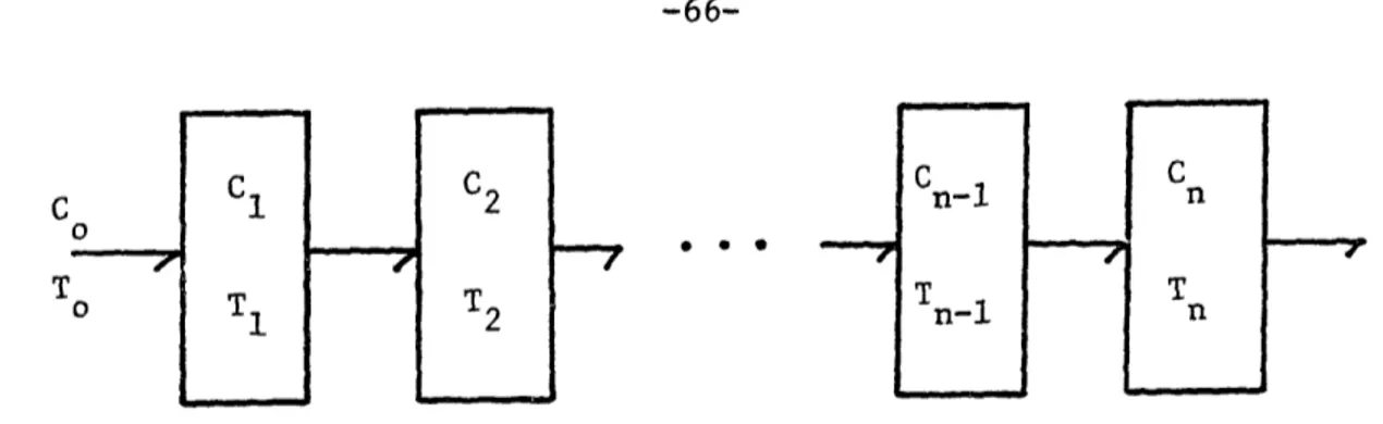
The combustion furnace element equations are formulated utilizing perfectly stirred reactor (PSR) theory. The steady state characteristics of a combustion chamber have been successfully represented, as described in

(34)

reference [11] using the PSR model. The extension of the PSR model for transient analysis is developed here for representation of combustion after a fuel trip.

In a perfectly stirred reactor as illustrated in Figure 2-3 incoming fuel is assumed to be dispersed uniformly throughout the reactor. The uniform fuel distribution assumption within a PSR reduces the theoretical requirements to an overall mass and energy balance on the reactor, plus a reaction rate equation per unit of reactor volume. The simplicity of the perfectly stirred model results from the neglect of spatial variations. The fuel concentration and temperature gradients in a large boiler furnace space thus must be represented by a number of PSR elements.

Both gas mass flow and fuel mass flow may be injected into a PSR. By the PSR assumption, the incoming materials are distributed instantaneously and uniformly throughout the PSR. In the process, they are mixed with and diluted by the materials already present. A unique gas density and an unburnt fuel concentration represent the mass states of the PSR. The unburnt fuel mass conservation can be expressed with the assumption that the unburnt fuel particles or droplets leave the PSR at the same speed as the exiting gas. The equation (2.4) implies that the rate of accumulation of unburnt fuel is equal to fuel flow into the PSR minus the fuel burning rate.

dC/dt = Wf/V + CiWi/piV - CW/pV - Rt (2.4)

where: C = concentration of inburnt fuel, lbm/ft3

Wf = fuel mass flow rate, lbm/sec. V = volume of PSR, ft3

(35)

I I

¢

Q

Figure 2-2: Plenum Volume Element

Wf

W T C

VQ

Figure 2-3: Perfect Stirred Reactor (PSR) Model for Combustion Furnace Wi Ti C, i. P,T,C

(36)

WO = gas mass fow rate, lbm/sec.

p = gas density, lbm/ft 3

Rt = combustion rate, lbm/(sec.ft3)

After combustion, part of the burnt fuel changes to a gaseous state according to the chemical reaction stoichiometry of the combustion process.

dM/dt = Wi + (1-f)VRt - Wo (2.5)

where: M = mass of gas in PSR, bm

W_i = gas flow rate entering PSR. bm/sec. 8f = fraction of ash in fuel

Application of first law of thermodynamics to the PSR results in the energy conservation equation:

dU/dt = E- Q + cpWiTi - cpWoT (2.6)

where: Ti = temperature of inlet gas flow, °R

T = temperature of PSR, °R

E = rate of energy conversion into gas, Btu/sec. Q = heat transfer rate leaving PSR. Btu/sec. U = internal energy in the PSR, Btu

cp= specific heat of gas at constant pressure

If the ideal gas law is assumed for the PSR combustion gas, then the internal energy U is a function of temperature T:

(37)

U = cMT (2.7)

where: M = the mass of the gas in the PSR

c_v = the specific heat of the combustion gas.

The specific heat of the combustion gas can be obtained from the Rosin-Fehling I.T. diagram shown in Figure 2-4 from reference [58]. The ideal gas law also defines the following relations, with the traditional qausi-static assumption for thermodynamics:

PV RMT (2.8)

Cp 1.4cv (2.9)

where: P = pressure in the PSR. lbf/ft2 R = ideal gas constant. lbf-ft/lbm°R

The energy into the combustion furnace gas model is equal to the energy generated by combustion minus the energy needed to heat and evaporate the moisture content in the fuel and gas:

E = E- Ew (2.10)

where: Ec = energy generated by combustion.

E, = energy needed to heat and evaporate moisture.

It has been shown that the combustion properties of normal commercial fuels can be fairly accurately specified by two parameters, namely, the caloric value and type of fuel. When the fuel burn rate is defined, the local rate of energy generation then may be defined as the product of fuel caloric value and

(38)

its burn rate. The total combustion rate in a PSR volume then becomes:

Ec = HVVRt (2.11)

A reaction rate equation which is a function of temperature and composition may be written as:

R_t = r(T) C₁ C2 (2.12)

where: C₁ = concentration of reactant 1 C₂ = concentration of reactant 2

r(T) = temperature dependency function

Since oil and pulverized coal are mainly of interest here, the general rate expressions are derived for these two cases in the following paragraphs.

(1) Oil Fired Combustion Rate Equation

In reference [4j Bragg and Holliday have derived the rate equation for oil combustion assuming that the concentration of two species participating in the oxidation of carbon monoxide are proportional to the concentration of the unburnt fuel and oxygen respectively as:

EV = kcP2T 3/2CoxC eB/RT (2.13)

where: Ev = local rate of energy release, Btu/sec.ft3

C = unburnt fuel concentration, lbm/ft3

Cox = Oxygen concentration, lbm/ft3 kc = collison frequency constant, 1/sec. T,P = local temperature and pressure

(39)

B = activation energy R = gas constant

Based on experimental results, a proedure to evaluate the value of B/R has been proposed in reference [4].

For implosion studies, the rate equation may be simplified. After a MFT, the fuel supply is reduced to zero in approximately one to two seconds, the fuel concentration change dominates the rate change during this process. When the the temperature drops as a result of the disturbance, the exponential term eB/RT dominates the combustion rate and a simple rate equation can be written in the form:

Rt = K eB/RT C (2.14)

This expression is combined with state equations (2.4),(2.5),(2.6) to simulate combustion dynamics after a MFT in oil fired plants.

(2) Pulverized Coal Fired Combustion Rate Equation

Pulverized coal combustion may be described as a five step reaction process:

- Step 1. Diffusion of gaseous reactant through the film surrounding the coal particle surface.

- Step 2. Penetration and diffusion of gas through the blanket of ash to the surface of the unreacted core, the reaction surface.

- Step 3. Chemical reaction of the gaseous reactant with the coal. - Step 4. Diffusion of the gaseous products through the film back into

(40)

- Step 5. Diffusion of the gaseous reaction product through the film back into the main gas body.

Since these steps must occur successively for the reaction to occur, they may be considered as resistances in series and whenever one of the steps offers the major resistance, that step may be considered as the rate controlling step. One important characteristic of the combustion rate is its temperature dependency. In different temperature ranges, different processes control the rate. The temperature dependency of pulverized coal combustion has been discussed in reference [58] and illustrated in Figure 2-5 where chemical reaction is rate controlling in the low temperature range and film and ash diffusion are rate controlling at higher temperatures. For low temperatures where the chemical reaction is controlling, the rate temperature dependency has been derived in reference [581 as:

rc = k2 eB/RT (2.15)

For high temperatures where mass transfer rate is controlling, the rate temperature dependency has been derived in reference [58] as:

rm = (PoDo/lf)(T/To) m < 2 (2.16)

where: Do = diffusion coefficient at a standard temperature To

if = film thickness

If a large temperature range is of interest, both mass transfer and chemical reaction require consideration and an overall rate may be derived as shown in reference [39] as:

(41)

4 C -W C w q) 0 U .-_cu 0 2 4: r-~-'ure (oC)

:ehling l.T. _{Diagram Ref. 55}

Chemical reacti,, ercentage Xcess Air ontrolling diffusio_n tance _ontrolling

Figure 2-5: Reaction Rate as a _{Function of Temperatu}

Iw .a: 4J -- -Z' Lin _{Gas T em pp --}_,_{# .} -i / -) 2000 Figure

(42)

if the rate of the chemical reaction alone is Rtl and the rate of mass transfer alone is Rt2.

In implosion studies, both mass transfer and chemical reaction are considered for coal fired combustion and the overall rate equation is used combining (2.15), (2.16) and (2.17) in the PSR model.

2.2.3 Transmission Line Element

Transmission line elements are used to represent wave propagation due to distributed inertance and capacitance of the fluid in the duct. A distributed parameter model of a lossless fluid transmission line is developed which represents the dominant longitudinal wave transmission modes in ducts. The model is derived for a duct of uniform cross section with rigid walls and assumes the flow is lossless with a fluid velocity small compared with the acoustic velocity of sound in the fluid. In most plant duct sections the average flow velocities are less than 5% of the acoustic sound velocity and the assumption that the flow velocity is small compared with the velocity of sound is valid. The model for a single line assumes that the temperature in the line is uniform. In sections of a plant where temperature varies significantly along the duct length, several lines each with a different temperature may be required to represent the complete line.

The application of the continuity and momentum equations to the elemental control volume of a fluid transmission line may lead to the derivation of two classical wave equations for pressure and mass flow rate representing the dynamic behavior of a single line.

(43)

a2W/ 2X = p//3 2W// 2t (2.19) The detailed derivation of equations (2.18) and (2.19) is summarized in Appendix A. For the time domain solution to these equations the pressure and

flow in the line can be represented by an alternate set of variables called wave scattering variables. The pressure waves in the line are partitioned into waves which travel in the flow direction, represented by U, and waves which travel opposite to the flow direction, represented by V. The pressure and flow at upstream and downstream ends of the line can be defined in terms of the wave scattering variables and charateristic impedance Z:

PU UU + VU (2.20)

WU (UU - VU)/ZC (2.21)

PD - UD + VD (2.22)

WD = (UD - VD)/ZC (2.23)

If the pressure is in inches of water and the mass flow rate is in pounds per second, the characteristic impedance is defined as:

Co

Z C (2.24)

A(32.2)(5.3)

The velocity of the sound C can be expressed as function of the duct line temperature as:

C_O = RT (2.25)

Using the scattering wave variables, the solutions to the wave equations (2.18) and (2.19) can be expressed in a very convenient form [21]. The

(44)

detailed derivation of this solution is also included in Appendix A.

UD(t) = UU(t-TD) (2.26)

VU(t) = VD(t-TD) (2.27)

The wave propagation delay is:

TD = L/C o (2.28)

The pressures and flows of the transmission line are expressed in terms of pure time delays. The time delay, TD, represents the time required for a pressure wave to travel the length of the line. Equation (2.26) shows that for the wave which travels downstream the downstream value of UD at time t is equal to the upstream value UU at time (t - TD) where the time difference is the time required for the wave to travel the length of the line. Similarly, for the upstream traveling wave, the upstream value of VU at time t is equal to the downstream value of VD at time (t -

TD)-A diagram of the transmission line model is shown in Figure 2-6. The wave variables UD and VU are considered quasi-state variables for the system since they define the state of the system and are related to the values of UU and VD by the delay TD. The characteristic impedance determines in part the portion of the wave reflected and transmitted when a line is coupled with another element and relates the wave variables to the pressures and mass flows at each end of the line. The delay TD and characteristic impedance Z which represent the characteristics of the transmission line, are function of transmission line parameters. In the thermal transient, the temperature of the duct changes with time. TD and Z also vary with time according to

(45)

equations (2.25), (2.28) and (2.24). These temperature (convective energy) dynamics of the duct are modeled by a global energy balance equation over the duct volume. The model is equavilent to coupling a plenum element with the volume size of the duct to the pressure - flow wave model. The flow rate input to this "duct plenum" is determined by the wave equations. Although it is not appropriate to assume a perfectly mixed fluid to compute the thermodynamic states in this dynamic situation, integration of the net mass and energy flows into this "duct plenum" will approximate the average gas density and temperature for the duct. In this type of the model formulation, a uniform but possibly time varying temperature is defined for a single transmission line.

The numerical solution of the wave equations, the values of UU and VD are established at time t by the equations coupling the line to the other elements in the system. Both pressure and flow are related to the scattering variables at the end of the transmission line as shown in Figure 2-6. The values of UD and VU at time t are then established directly from the values of UU and VD by the delay operator. The average temperature of the duct is obtained by integrating the net incoming energy flow. The parameters TD and -Z c also vary with temperature and are updated when a thermal disturbance occurs upstream. However, the heat transfer along the duct is not considered, such a topic is discussed with other dispersion effects in references [25] [5] and

[6].

2.2.4 Centrifugal Fan Element

The generic representation of a centrifugal fan element is by a steady state pressure-flow relation :

(46)

CZ_o a) an ca 0. C PJ ,4 o a) r4

(47)

P = F( W, a ) (2.29)

where F(W,a) is the functional relationship relating flow W and fan inlet guide vane or damper angle a to pressure rise AP.

This fan relation may be defined in general in terms of a dimensionless flow coefficient () and a dimensionless pressure coefficient . These coefficients are derived by dimensional analysis to fans with geometric similarity. When -' the Reynolds number does not vary significantly, the functional relationship

'TI = ff(4,a) (2.30)

represents the general characteristics of geometricaly similar fans, where the coefficients are defined as:

4_Qf ird2u (2.31) trd2u 2AP = 2 (2.32) pu

where: d = fan impeller diameter u = impeller tip speed Qf = volume flow rate

p = fluid density

AP = pressure rise across the fan

The symbolic representation and typical centrifugal fan characteristics are shown in Figure 2-7 and Figure 2-8 respectively. The normalized fan curves in Figure 2-8 are characterized at M.I.T. [59].

For numerical work the function ff(W,a) is either represented as a table with pairs of values of AP and W for fixed a or with a polynomial fit to

(48)

Figure 2-7: Centrifugal Fan Symbolic Representation - 100 = 25° = 400 = 550 0.0 0.1 0.2 0.3 0.4 0.5 0.6 0.7 0.8

Figure 2-8: Typical Centrifugal Fan Characteristics 1.2 1.1 1.0 0.9 0.8 0.7 0.6 0.5 0.4 0.3 0.2 0.1 0.0 _ 1 ____~~~~~~~~~~

(49)

equation (2.33). For each fixed angle a, a polynomial can be determined by the least squares method:

I = ECJ4i (2.33)

For different angles a, a different set of coefficients Ci are obtained so that the polynomial coefficients in (2.33) are functions of the angle a. This functional relation can also be approximated as polynomials:

C i= bi jaJ (2.34)

By substituting equation (2.34) into (2.33), the numerical approximation of the fan characteristics is established as:

4I = Zbjjaj4 ; (2.35)

2.2.5 Axial Fan Element

The generic representation of an axial fan element is by a steady state pressure-flow relation:

AP = Fa( W, c ) (2.36)

where Fa(W,a) is the functional relationship relating flow W and fan blade or damper angle a to pressure rise AP.

This fan relation may be defined in general in terms of a dimensionless flow coefficient and a dimensionless pressure coefficient A. These coefficients are derived by dimensional analysis to fans with geometrical similarity. When the Reynolds number does not vary significantly, the functional relationship

(50)

represents the general characteristics of geometrical similar fans, where the coefficients are defined as:

4Qf -r 2 (2.38) lrd2u 2AP =1 2 (2.39) pu

where: d = fan impeller diameter u = impeller tip speed Qf = volume flow rate

p = fluid density

AP = pressure rise across the fan

The symbolic representation of an axial fan and typical axial fan characteristics are shown in Figure 2-9 and Figure 2-10 respectively.

For numerical work the function fa(Wa) is either represented as a table with pairs of values of AP and W for fixed a or with a polynomial fit to the fan curves. Because of the stall characteristic of the axial fan curve, a piecewise curve fit is usually preferred rather than a full range one. For each fixed angle a, a polynomial can be determined by the least squares method just as shown in the centrifugal fan case.

Since the mass flow passes through a relative long ring-section chamber of an axial fan, the gas flow inertance effect becomes important and should be included in the model by the following equation:

I(dW/dt) = API (2.40)

(51)

Figure 2-9: Axial Fan Symbolic Representation

Blade angle

(52)

I =La/Aa

La = length of the axial fan chamber

A_a = cross section area of axial fan chamber

2.2.6 Flow Resistance Element

The symbolic representation of the resistance element is shown in Figure 2-11, it represents the quasi-steady pressure-drop/flow characteristics of ducts, bends and other equipment and may be represented as the functional relationship:

Ap-= f(W) (2.41)

The functional relation of equation (2.41) for a straight duct can be expressed as:

AP = fArTIWIW

(2.42)

where f is the friction coefficient and is a function of the flow Reynolds number, and Ar is a geometry coefficient and is a function of duct length and cross section area. For most power plant applications Ar is constant, and f is assumed constant since most flows are in the turbulent region. The temperature T is the weighted average of the upstream temperature and the downstream temperature of the duct representing the effect of the gas density change due to compressibility and heat transfer along the duct. Under these conditions, the pressure drop AP is proportional to fluid absolute average temperature T (R) and mass flow squared IWIW:

(53)

AP = kg T WIW (2.43)

Equation (2.43) is valid not only for straight ducts but also for bends, tube banks, dampers, airheaters and other equipment with some modifications of the coefficient kg. Analytical and empirical expressions for kg are given in reference [7].

2.2.7 Mechanical Damper Element

A mechanical damper is one type of fluid resistance which deserves attention because of its relation to draft control. The symbolic representation of a mechanical damper is shown in Figure 2-12. The generic characteristic is represented by a pressure-flow relation with the damper angle as a parameter:

AP = Df( W, ad ) (2.44)

The particular functional relation in (2.44) is provided by manufacturers curves or tables where pairs of values for AP and W for a fixed a d are listed. For numerical work the function (2.44) can be approximately represented by a polynomial using the least squares method:

AP = Eri(ad)W (2.45)

2.2.8 Heat Transfer Resistance Element

The heat transfer resistance element represents heat transfer between two objects. The symbolic representation is shown in Figure 2-13.

(54)

Figure 2-11: Symbolic Representation of Resistance Element

(55)

There are three recognized modes of heat transfer, conduction, convection and radiation. All the varied phases of heat transfer involve one or more of these modes. For the conduction mode:

k

Q = -Ah(T1-T 2)

where: Q = rate of heat flow, Btu/hr

k = thermal conductivity. Btu/ft2 hr.F/ft A_h = heat transfer area, ft2

1 = thickness, ft

Convection heat transfer between a fluid and a solid is expressed as Q = UcAh(T - T2)

where U is the convection film conductance, Btu/ft2_,hr,F.

Radiation heat transfer in combustion furnaces is defined as:

Q =- Ah (faT 4 - oETs4)

where:

a = Stefan-Boltzmann constant f = flame emissivity

E = ash deposit emissivity

a = ash deposit absorptivity

(2.47)

(2.48)

(56)

2.2.9 Solid Thermal Element

In order to study the thermal transient problem after a MFT, a good estimation of the energy storage in plant structures and in slag is important. These metal structures and ash slags can be modeled as solid thermal elements illustrated in Figure 2-14. The consitutive equation for this element is:

cMsdT/dt = Q (2.50)

where: c = specific heat for the solid Ms = mass of the solid

Q = heat transfer into the element T = solid temperature

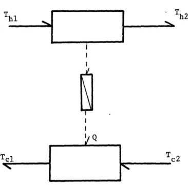
2.2.10 Heat Exchanger Element

The heat transfer and energy exchange at the superheater, economizer and airpreheater can be modeled with heat exchanger elements. The symbolic representation of the heat exchanger element is shown in Figure 2-15. The exact heat transfer solutions are available for both counter-flow and parallel-flow exchangers as given in reference [50].

ATa - ATb

Q = UA (2.51)

Ln(ATa/ATb) The hot side energy flow is:

hh = ChW[Thl+Th2]/2 + ChlWhl[Thl-Th2]/2 Q (2.52)

(57)

Figure 2-13: Heat Transfer Element