Alternatives to the gradient in optimal transfer line buffer allocation

Alternatives to the Gradient in Optimal Transfer

Line Buffer Allocation

by

Ketty Tanizar

B.S., Industrial Engineering and Operations Research

University of California at Berkeley, CA, 2002

Submitted to the Sloan School of Management

in partial fulfillment of the requirements for the degree of

Master of Science in Operations Research

at the

MASSACHUSETTS INSTITUTE OF TECHNOLOGY

September 2004

( Massachusetts Institute of Technology 2004. All rights reserved.

P

-Author ...

...

.

Sloan School of Management

August 13, 2004

,-, /_

r

Certified by...

Senior Research Scientist,

.eptanley

B. Gershwin

Department of Mechanical Engineering

Thesis Supervisor

Accepted

by

...

.-

. ..

7

James B. Orlin

Co-Directors, Operations Research Center

Alternatives to the Gradient in Optimal Transfer Line Buffer

Allocation

Ketty Tanizar

Submitted to the Sloan School of Management

on August 13, 2004, in partial fulfillment of the requirements for the degree of

Master of Science in Operations Research

Abstract

This thesis describes several directions to replace the gradient in James Schor's gradi-ent algorithm to solve the dual problem. The alternative directions are: the variance

and standard deviation of buffer levels, the deviation of the average buffer level from

half-full, the difference between probability of starvation and blocking, and the dif-ference between the production rate upstream and downstream of a buffer. The objective of the new algorithms is to achieve the final production rate of the dual problem faster than the gradient. The decomposition method is used to evaluate the

production rates and average buffer levels. We find that the new algorithms work

better in lines with no bottlenecks. The variance and standard deviation algorithms

work very well in most cases. We also include an algorithm to generate realistic

line parameters. This algorithm generate realistic line parameters based on realistic constraints set on them. This algorithm does not involve filtering and is fast and reliable.

Thesis Supervisor: Stanley B. Gershwin

Acknowledgments

First I would like to thank Dr. Stanley Gershwin for being a terrific advisor and a great friend. I thank him for his trust in me and for constantly challenging me.

I would like to thank Chiwon Kim, Youngjae Jang, Jongyoon Kim, and Zhenyu Zhang for being great friends and colleagues. I will always be grateful for all the

discussions we had and most of all for our beautiful friendship.

I would also like to thank my fellow ORC S.M. students: Kendell Timmers,

Christopher Jeffreys, Corbin Koepke, and Sepehr Sarmadi for being the best study

mates I could ever ask for. Our study sessions and stimulating discussions were certainly one of the most enjoyable parts of my M.I.T. experience.

I want to give special thanks to Hendrik, Leonard, Doris, and Liwen for always taking the time to listen and for accepting me the way I am. Also, I would like to

thank Rudy and Andrea for making me laugh. I could not ask for better friends.

In closing, I would thank my mother, my father, and my sister Nelly for their

Contents

1 Introduction

1.1 General Problem Description ... 1.2 Approach ...

1.3 Literature Review .

1.3.1 Qualitative Properties of the Line 1.3.2 Characteristics of the Solutions 1.3.3 Some Solutions Approaches . . . 1.3.4 Preliminary Work . . . . . . .. . . . . . . . Performance . . .. . . . . . . . . . . . .. . . . .

2 Technical Problem Statement

2.1 Definitions and Properties ... 2.1.1 Parameters and Notation .. 2.1.2 Qualitative Properties . 2.2 Model Type and Problem Types . .

2.2.1 Model Type...

2.2.2 Decomposition Algorithm 2.2.3 Problem Types ... 2.3 Review of Schor's Dual Algorithm .

3 Variability and Optimality

3.1 Intuitive Justification ...

3.2 Motivations of the New Directions ... 3.3 Derivation of the New Algorithms ...

19 19 20 20 20 21 21 22 27 27 27 28 28 28 30 32 33 37 37 40 43 . . . . . . . . . . . . . . . . . . . . . . . . . . . .

...

...

...

...

...

...

...

...

4 Performance of the New Algorithms

4.1 Accuracy ...

4.1.1 Identical versus Non-Identical Lines ...

4.1.2 The Location, Existence, and Severity of Bottlenecks 4.2 Reliability ...

4.2.1 Identical Machine Lines ... 4.2.2 Non-Identical Machine Lines ... 4.3 Speed ...

4.3.1 Identical Machine Lines ... 4.3.2 Non-Identical Machine Lines ...

5 Sensitivity Analysis

5.1 Identical Machine Lines ....

5.2 Non-Identical Machine Lines . .

6 Conclusion and Future Research

6.1 Conclusion ... 6.1.1 Accuracy. 6.1.2 Reliability ... 6.1.3 Speed ... 6.1.4 Sensitivity Analysis . . . 6.2 Future Research ...

A Generating Realistic Line Parameters

A.1 Motivation ...

A.2 Realistic Constraints on Parameters ... A.3 Implementation ...

A.3.1 Difficulties with Filtering ...

A.3.2 Generating Lines with non-Bottleneck Machines A.3.3 Generating Lines with Bottleneck Machines . . A.4 Example ... 47 47 48 51 58 60 62 62 63 63 69 69 70 79 79 79 80 80 80 81 83 83 83 86 86 87 92 94 . . . . . . . . . . . . . . . . . . . . . . . . . . . . . . . . . . . .

...

...

...

...

...

...

...

...

A.5 Conclusion ... 94

B Linear Search to Find the Next Point on the Constraint Space

97

B.1 Binary Search ... 97

List of Figures

1-1 Test Result: 60% Efficiency with 0% Variations in r and p Values .. 23

1-2 Test Result: 96% Efficiency with 15% Variations in r and p Values .. 23

1-3 Test Result: 91% Efficiency with Bottleneck and with 15% Variations in r and p Values ... 24

1-4 Values of Gradient i, Variance i, Standard Deviation i, Ii- 1, pb(i)-ps(i), and Pu(i) - Pd(i)l at the Optimal Buffer Allocation ... 25

1-5 Values of 1 , and at the Optimal Buffer Al-location ... 26

2-1 Transfer Line ... 27

2-2 Decomposition of Line ... 31

2-3 Block Diagram of Schor's Algorithm . ... 34

2-4 Constraint Space ... 36

3-1 The Gradient and the Projected Gradient Vectors . ... 41

3-2 Types of Computations Calculated at Each Optimization Step .... 42

3-3 Block Diagram of the New Algorithms . ... 44

4-1 Final P of the Other Directions as Proportions of Final P of the Gra-dient in the Identical Machine Case ... 48

4-2 Final Two-Machine Line Counter of the Other Directions as Propor-tions of Final Two-Machine Line Counter of the Gradient in the Iden-tical Machine Case ... 49

4-3 Production Rate versus Two-Machine Line Counter for an Identical

Machine Case ... 50

4-4 Final P of the Other Directions as Proportions of Final P of the Gra-dient in the Non-Identical Machine Case ... 51 4-5 Final Two-Machine Line Counter of the Other Directions as

Propor-tions of Final Two-Machine Line Counter of the Gradient in the

Non-Identical Machine Case ... 52

4-6 Final P of the Other Directions as Proportions of Final P of the Gra-dient Algorithm in Short Lines with Bottlenecks ... 53 4-7 Final Two-Machine Line Counter of the Other Directions as

Propor-tions of Final Two-Machine Line Counter of the Gradient Algorithm in Short Lines with Bottlenecks ... .. 53 4-8 Final P of the Other Directions as Proportions of Final P of the

Gra-dient Algorithm in Short Lines with No Bottlenecks ... 54 4-9 Final Two-Machine Line Counter of the Other Directions as

Propor-tions of Final Two-Machine Line Counter of the Gradient Algorithm

in Short Lines with No Bottlenecks ... 55

4-10 Final P of the Other Directions as Proportions of Final P of the Gra-dient Algorithm in Long Lines with Bottlenecks ... 55 4-11 Final Two-Machine Line Counter of the Other Directions as

Propor-tions of Final Two-Machine Line Counter of the Gradient Algorithm

in Long Lines with Bottlenecks ... .. 56

4-12 Final P of the Other Directions as Proportions of Final P of the

Gra-dient Algorithm in Long Lines with No Bottlenecks ... 56

4-13 Final Two-Machine Line Counter of the Other Directions as Propor-tions of Final Two-Machine Line Counter of the Gradient Algorithm

in Long Lines with No Bottlenecks ... 57

4-14 Final P of the Other Directions as Proportions of Final P of the

Gra-dient Algorithm in Identical Machine Lines with One Mild Bottleneck

4-15 Final P of the Other Directions as Proportions of Final P of the Gra-dient Algorithm in Identical Machine Lines with One Mild Bottleneck

Located in the Middle of the Line ... . 58 4-16 Final P of the Other Directions as Proportions of Final P of the

Gra-dient Algorithm in Identical Machine Lines with One Mild Bottleneck

Located Downstream . . . ... 58

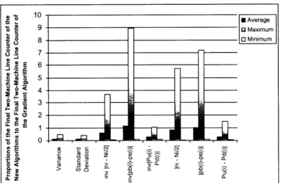
4-17 Final Two-Machine Line Counter of the Other Directions as Propor-tions of Final Two-Machine Line Counter of the Gradient Algorithm

in Identical Machine Lines with One Mild Bottleneck Located Upstream 59

4-18 Final Two-Machine Line Counter of the Other Directions as Propor-tions of Final Two-Machine Line Counter of the Gradient Algorithm

in Identical Machine Lines with One Mild Bottleneck Located in the

Middle of the Line ... 60

4-19 Final Two-Machine Line Counter of the Other Directions as Propor-tions of Final Two-Machine Line Counter of the Gradient Algorithm in Identical Machine Lines with One Mild Bottleneck Located Downstream 61 4-20 Final P of the Other Directions as Proportions of Final P of the

Gradi-ent Algorithm in IdGradi-entical Machine Lines with One Severe Bottleneck

Located Upstream .. . . . ... 61

4-21 Final P of the Other Directions as Proportions of Final P of the Gra-dient in the Identical Machine Case, with Equal Initial Buffer Allocation 62 4-22 Final P of the Other Directions as Proportions of Final P of the

Gra-dient in the Identical Machine Case, with Initial Buffer Allocation

Pro-portional to _{Pi+Pi+l ...}1 63

4-23 Final P of the Other Directions as Proportions of Final P of the Gradi-ent in the IdGradi-entical Machine Case, with Random Initial Buffer Allocation 64 4-24 Final P of the Other Directions as Proportions of Final P of the

Gra-dient in the Non-Identical Machine Case, with Equal Initial Buffer Allocation ... 65

4-25 Final P of the Other Directions as Proportions of Final P of the Gra-dient in the Non-Identical Machine Case, with Initial Buffer Allocation

Proportional to _{pi+ pi+} 1 _{. . . ..} 65

4-26 Final P of the Other Directions as Proportions of Final P of the Gra-dient in the Non-Identical Machine Case, with Random Initial Buffer Allocation ... 66

4-27 Final Two-Machine Line Counter as Line's Length Increases in the

Identical Machine Case ... 66

4-28 Production Rate versus Two-Machine Line Counter for an Identical

Machine Case with k = 42 ... 67

4-29 Final Two-Machine Line Counter as Line's Length Increases in the

Non-Identical Machine Case ... 67

5-1 Sensitivity Results of the Gradient Algorithm on Identical Machine Lines 70

5-2 Sensitivity Results of the Variance Algorithm on Identical Machine Lines 71

5-3 Sensitivity Results of the Standard Deviation Algorithm on Identical

Machine Lines . . . ... 72

5-4 Sensitivity Results of the

----

5-5 Sensitivity Results of the _Ipb(i)-p(i)I1 Algorithm on Identical Machine

Lines ... 73

5-6 Sensitivity Results of the _IP,(i)-Pd()I1 Algorithm on Identical Machine

Lines ... 73

5-7 Sensitivity Results of the I- -Ni Algorithm on Identical Machine Lines 74

5-8 Sensitivity Results of the Ipb(i) -p(i)l Algorithm on Identical Machine

Lines ... 74

5-9 Sensitivity Results of the I P, (i) -Pd(i) I Algorithm on Identical Machine

Lines

...

...

75

5-10 Sensitivity Results of the Gradient Algorithm on Non-Identical

5-11 Sensitivity Results of the Variance Algorithm on Non-Identical

Ma-chine Lines ... ... 76

5-12 Sensitivity Results of the i Algorithm on Non-Identical Machine Lines ... 77

A-1 Upper Bounds, Lower Bounds, and the Values of r Generated .... 94

A-2 Upper Bounds, Lower Bounds, and the Values of p Generated .... 95

A-3 Upper Bounds, Lower Bounds, and the Values of pl Generated .... 95

B-1 N'in,N ma and fl on the Constraint Space for k = 4 ... 99

B-2 a*i,, a*ax, and the Production Rate Function along the Line Parallel to for k = 4 ... 99

B-3 Locations of tempamin, tempaminmid, tempamid, tempamidmax, tempamax 101 B-4 Locations and Values of Pamin, Paminmid, Pamid,Pamidmax, and Pamax 102 B-5 A Monotonically Increasing Production Rate Function ... 103

B-6 The New amin, amid, and amax for the Monotonically Increasing Functionl04 B-7 A Monotonically Decreasing Production Rate Function ... 104

B-8 The New amin, amid, and amax for the Monotonically Decreasing Function105 B-9 A Strictly Concave Production Rate Function . ... 106

B-10 The New Collapsed Region for the Strictly Concave Inner Production Rate Function: New Collapsed Region . ... 107

B-11 New Collapsed Region ... 109

B-12 Another New Collapsed Region ... .. 110

B-13 The Final Collapsed Region ... 111

List of Tables

1.1 The Line Parameters for Figure 1-4 and Figure 1-5 ... 25

3.1 Direction Computation Comparisons for the Different Methods .... 42 4.1 The Line Parameters of which Results are Shown in Figure 4-3 . . . . 50

4.2 The Line Parameters of which Results are Shown in Figure 4-28 . . . 64 5.1 The Original Line's Parameters Used in Sensitivity Analysis of

Identi-cal Machine Lines ... 69

5.2 The Original Line's Parameters Used in Sensitivity Analysis of

Non-Identical Machine Line ... 75

A.1 Comparisons between the Performance of the Filtering Algorithm and the Performance of the New Algorithm in Generating a Line with k

Chapter 1

Introduction

1.1 General Problem Description

In this paper, we focus on buffer optimization of a production line. A production

line, or flow line, or transfer line is a manufacturing system where machines or work

centers are connected in series and separated by buffers. Materials flow from the upstream portion of the line to the first machine, from the first machine to the first buffer, from the first buffer to the second machine, and continue on to the downstream portion of the line.

There are two types of buffer optimization problems. The first one, or the primal problem, is to minimize the total buffer space in the production line while trying to achieve a production rate target. This problem is usually encountered when the available factory space is limited. The other problem, or the dual problem, is to max-imize production rate subject to a specified total buffer space. The second problem

is encountered when floor space is not a problem and the major goal is to achieve as high production rate as possible. In both problems, the size of each buffer becomes

the decision variable.

Schor uses a gradient method to solve the dual problem and solve the primal problem using the dual solution [SchorOO]. Although the gradient approach proves to

be very efficient, it can be time-consuming. We propose using different approaches

1.2 Approach

In this paper, we focus on solving the dual problem. Therefore, the question we are

asking is: given the machines of a transfer line and a total buffer space to be allocated, how should we allocate buffer space so that the production rate is maximized? We begin our paper by describing some work in the area of buffer optimization (Chapter

1).

In Chapter 2, we define some parameters and notation used throughout the paper. We also mention some qualitative properties assumed about transfer lines. Finally, we describe the primal and the dual problem quantitatively and review the Schor's gradient algorithm for solving the dual problem.

The purpose of the paper is to examine some alternative directions, other than the gradient, to use in solving the dual problem. In Chapter 3, we mention an intuitive justification and motivation for using the alternative directions. The new algorithms are also derived in Chapter 3.

We review the performance of the new algorithms, in terms of accuracy, reliability, and speed, in Chapter 4. In Chapter 5, we perform a sensitivity analysis of the new algorithms if the machine parameters are varied by a small amount. Chapter 6

discusses the conclusion and future research.

We also include two appendices. Appendix A describes an algorithm to generate

realistic line parameters. This algorithm generates r,p, and At based on realistic constraints set on them. It avoids any filtering and is, therefore, fast and reliable.

Appendix B describes the linear search method used in the new algorithms.

1.3 Literature Review

1.3.1 Qualitative Properties of the Line Performance

In order to develop algorithms relevant to transfer lines, we need to understand the behavior of the lines. One aspect of the behavior is how the production rate of the line

the production rate increases as each buffer size is increased. However, the increase in production rate becomes less significant as the buffer size increases. This is shown

by Meester and Shanthikumar [Meester90O], who proved that the production rate is

an increasing, concave function of the buffer sizes.

1.3.2 Characteristics of the Solutions

The purpose of this paper is to propose alternative directions that can be used to replace the gradient in Schor's dual algorithm [Schor0]. One paper that motivates two alternative directions used in this paper is the paper by Jacobs, Kuo, Lim and Meerkov [Jacobs96]. Jacobs et al. did not suggest a method to design a manufacturing system, but instead proposed a method of improving an existing system using data that is available as the system runs. They used the concept of "improvability" (similar to "non-optimality" but used in the context when optimality may be impossible due

to the lack of precise information on the factory floor) to determine how buffer space

should be allocated. Jacobs et al. showed that a transfer line is unimprovable with

respect to work force if, each buffer is, on the average, half-full and if the probability

that Machine Mi is blocked equals the probability that Machine Mi+1 is starved.

1.3.3 Some Solutions Approaches

One approach to buffer size optimization is done by means of perturbation analysis. Ho, Eyler, and Chien [Ho79] were pioneers of this simulation-based technique. In this

paper, Ho et al. estimated the gradient of the production rate of a discrete-event dynamic system (one with discrete parts, identical constant processing times, and geometrically distributed repair and failure times) with respect to all buffer sizes,

using a single simulation run.

Another approach is by means of dynamic programming. Chow [Chow87]

devel-oped a dynamic programming approach to maximize production rates subject to a total buffer space constraint.

prob-lems. Park [Park93] proposed a two-phase heuristic method using a dimension re-duction strategy and a beam search method. He developed a heuristic method to minimize total buffer storage while satisfying a desired throughput rate.

Another approach to buffer allocation problem is by Spinellis and Papadopoulos

[SpinellisOO]. They compared two stochastic approaches for solving buffer allocation problem in large reliable production lines. One approach is based on simulated

an-nealing. The other one is based on genetic algorithms. They concluded that both methods can be used for optimizing long lines, with simulated annealing producing more optimal production rate and the genetic algorithm leading in speed.

Finally, an approach closest to our algorithm is Gershwin and Schor's gradient algorithm [SchorOO]. They used a gradient method to solve the problem of maximizing production rate subject to a total buffer space constraint (the dual problem) and used the solution of the dual problem to solve the primal problem.

1.3.4 Preliminary Work

The intuition behind using the alternative directions to substitute the gradient is supported by the following preliminary numerical and simulation studies:

1. A study about the relationship between optimum buffer allocation and buffer

level variance in a finite buffer line

In this study [KinseyO2], several machine lines with different machine param-eters and efficiencies are generated. The different machines are generated by

starting with some center values for r, p, and 1t. Later, a random number gener-ator is used to produce some variations for r, p, and p1 around their center values.

In some of the lines, a bottleneck is introduced by imposing a particularly low efficiency on a selected machine in the line. Finally, the correlation between the

optimal buffer allocation and standard deviation of buffer level is calculated. The following graphs show the optimal buffer sizes and the standard deviation

Figure 1-1 shows the result of the study for a twenty-identical-machine line with

a 60% efficiency level. The R2 value of the correlation between the optimal buffer sizes and the standard deviation of the buffer levels is 0.99.

Figure 1-1: Test Result: 60% Efficiency with 0% Variations in r and p Values

Figure 1-2 shows the result for a twenty-machine line with a 96% efficiency level

and with 15% variations in r and p values. The R2 value is 0.75.

Figure 1-2: Test Result: 96% Efficiency with 15% Variations in r and p Values

Figure 1-3 shows the result for a twenty-machine line with a 91% efficiency level

and with 15% variations in r and p values. For this line, Machine Mll is the

bottleneck. The R2 value of the correlation is 0.98.

This study concludes that the standard deviation of the buffer levels are well-correlated with the sizes of the buffers in optimized lines. In addition,

bot-120 100 80 60 40 20 0 1 2 3 4 5 6 7 8 9 10 11 12 13 14 15 16 17 18 19 Machine Number

- Optimal Buffer Size

200 .-- Standard Deviation of

Buffer Level

100

...

1 2 3 4 5 6 7 8 9 10 11 12 13 14 15 16 17 18 19

Figure 1-3: Test Result: 91% Efficiency with Bottleneck and with 15% Variations in

r and p Values

tlenecks in the machine line do not affect the correlation. This confirms the

hypothesis that the best place to put space is where variation is the greatest. 2. A study about the values of all directions at the optimal buffer allocations

calculated using the gradient method

In this study, the values of gradient i, variance i, standard deviation i of buffer

levels, W--iI, _{2 1, luo\fF I,-~v/l, I' U\"/} jpb(i)-Ps(i)I, jP(i)-Pd(i)j, I' _{~a\YJi ' pb(i)-s(i)1} l 1

and

are calculated at the optimal buffer allocation, obtained by the gradient algo-rithm.

Figure 1-4 shows an example of the normalized values of gradient i, variance

i, standard deviation i,

ni

point.

Figure 1-5 shows an example of the normalized values of . 1 and

lUP1 at the optimal point.

IPU(i)-Pd(i)I

Table 1.1 shows the data used to generate the results shown in Figure 1-4 and

Figure 1-5.

Figure 1-4 and Figure 1-5 show that gradient i, variance i, standard deviation i

of buffer levels, I- - 1 and have the same shapes as the

350 300 250 200 150 100 50 0 1 2 3 4 5 6 7 8 9 10 11 12 13 14 15 16 17 18 19 Machine Number

1.2

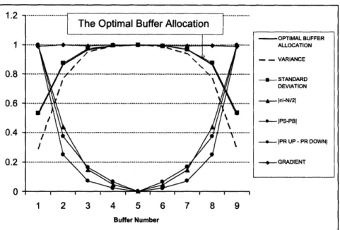
Figure 1-4: Values of Gradient i, Variance i, Standard Deviation i, 5i - I , pb(i) -ps(i)j, and IP,(i)- Pd(i)l at the Optimal Buffer Allocation

Table 1.1: The Line Parameters for Figure 1-4 and Figure 1-5

shape of the optimal buffer allocation. Therefore, these directions can be used

to allocate buffer sizes.

Figure 1-4 shows that ni I 1, pb(i)-ps(i)t, and IP.(i)-Pd(i)l have shapes that are inverse the shape of the optimal buffer allocation. Although their shapes are inverse the shape of the optimal buffer allocation, Ii - I, I -pb(i)- Ps(i),

and IP,(i) - Pd(i)l can also be used to allocate buffer sizes. The reason for this

will be explained in Chapter 3.

1 0.8 0.6 0.4 0.2 0 1 2 3 4 5 6 7 8 9 Buffer Number OPTIMAL BUFFER ALLOCATION - - VARIANCE --- STANDARD DEVIATION , Ini-Ni121 -- IjPS-PB[ -- PR UP - PR DOWNI - GRADIENT

Number of Machines 10 identical machines

Total Buffer Spaces to be Allocated 900 Repair Rate r 0.015 Failure Rate p 0.01

1.2 1 0.8 0.6 0.4 0.2 0 - OPTIMAL BUFFER ALLOCATION

1-- INVERSE Ini - Ni/21

-*- INVERSE IPS-PBI

-- INVERSE PR UP

-PR DOWNI

1 2 3 4 5 6 7 8 9

Buffer Number

Figure 1-5: Values of I pb()(i)l and I (i)-Pd(i)l at the Optimal Buffer

Chapter 2

Technical Problem Statement

2.1 Definitions and Properties

2.1.1 Parameters and Notation

In this research, we attempt to find the optimal buffer allocation of a production line, such that the production rate P of the line is maximized. The production line has k machines and k - 1 buffers. Ni is the size of Buffer Bi and ni is

the average buffer level of Buffer Bi. The production rate of the line P is a

function of the buffer sizes (N1,..., Nk1). Therefore, it is sometimes denoted

as P(N1, N2, N3, ..., Nk-1). Figure 2-1 shows a diagram of a transfer line with k

- 3, in which squares represent machines, circles represent buffers, and arrows

represent the work flow from the upstream portion of the line to the downstream portion of the line.

Figure 2-1: Transfer Line

When any machine upstream of Buffer Bi breaks down, that machine can not produce any parts. Eventually there are no parts coming into Buffer Bi so Buffer

Bi will be empty. Since Buffer Bi is empty, there are no parts to be processed

by machines downstream of Buffer Bi. This phenomenon is called starvation. Likewise, when any machine downstream of Buffer Bi breaks down, it stops

producing parts. Eventually Buffer Bi will be full because it can not transfer parts to the machine downstream of it. This causes the machine upstream of Buffer Bi to stop transferring parts to Buffer Bi because Buffer Bi can not hold the parts. This phenomenon is called blockage.

2.1.2 Qualitative Properties

* Continuity

A small change in Ni results in a small change in P.

* Monotonicity

The production rate P increases monotonically as Ni increases, provided all other quantities are held constant.

* Concavity

The production rate P is a concave function of (N1, ..., Nk-1).

2.2 Model Type and Problem Types

2.2.1 Model Type

There are three types of manufacturing systems models: * Discrete Material, Discrete Time

* Discrete Material, Continuous Time * Continuous Material Flow

The details of each model can be found in [Gershwin94]. In this paper, we use

the continuous material flow model.

In the continuous flow model, material is treated as though it is a continuous fluid. Machines have deterministic processing time but they do not need to have equal processing times. The failure and repair times of machines are exponentially distributed. There are three machine parameters in this model. The first one is the failure rate pi. The quantity piJ is the probability that Machine Mi fails during an interval of length while it is operating and the upstream buffer is not empty and downstream is not full. The second parameter is the repair rate ri. The quantity rid is the probability that the Machine Mi gets fixed while it is under repair during an interval of length 6. Finally, the last parameter is the operation rate pi. The quantity li is the processing speed of Machine Mi when it is operating, not starved or blocked, and not slowed down by an adjacent machine. The quantity i6 is the amount of material processed by Mi during an interval of length . As in the discrete material models, the

size of Buffer Bi is Ni. All ui, Pi, ri, and Ni are finite, nonnegative real numbers. The isolated efficiency of Machine Mi, denoted by ei, is the efficiency of Machine

Mi independent of the rest of the line. The isolated efficiency ei is defined

mathematically as

ri ei=

ri + Pi

In the continuous flow model, pi is the processing rate of Machine Mi when it is

operating, not starved or blocked, and not slowed down by an adjacent machine. Since Machine Mi's actual production rate is influenced by its efficiency, the

isolated production rate pi of Machine Mi is defined as

2.2.2 Decomposition Algorithm

When there are more than two machines in a transfer line and all Ni are

nei-ther infinite or zero, the production rate of the line and the average inventory levels of buffers can not be calculated analytically. This is where the decom-position algorithm plays an important role to approximate the production rate

and the average inventory levels, which otherwise can not be calculated. More specifically, ADDX algorithm [Burman95] is used to evaluate P and i when

the system is modeled using the continuous flow model. The ADDX algorithm uses analytical methods and decomposition method [Gershwin87] to determine approximate solutions.

The following is a brief description of the decomposition algorithm. Decom-position algorithm approximates the behavior of a k-machine line with k - 1

hypothetical two-machine lines, as illustrated in Figure 2-2 for k = 4. L(i)

represents the hypothetical two-machine line i. The parameters of L(i) are es-timated such that the flow of materials into Buffer Bi in L(i) approximates the

flow of materials into Buffer Bi in the original line L.

Machine MU(i) and Machine Md(i) represents the machine upstream and

ma-chine downstream of Buffer Bi in the artificial two-mama-chine line model. The

quantity r (i), i = 1, ..., k- 1, represents the repair rate of MU(i). The quantity

rd(i) represents the repair rate of Md(i). p(i) represents the failure rate of

Machine M,(i) and pd(i) represents the failure rate of Machine Md(i). Finally,

ju(i) represents the processing rate of Machine MU(i) and pd(i) be the

process-ing rate of Machine Md(i). The decomposition method works by calculatprocess-ing r.(i), rd(i), pu(i), pd(i), iuz(i), and d(i).

The starvation and blockage phenomena in the decomposition are defined as the starvation of Machine Md(i) and the blockage of Machine MU(i). More

specifically, ps(i) is defined as the probability of starving of Machine Md(i) and

pb(i) is defined as the probability of blocking of Machine MU(i).

M, B, M2 B2 M3 B3 M4 Original Line L r, N, r2 N₂ r₃ N3 r4 P1 P2 P3 P4 mu, mu2 mu3 mu4 Mu(1) B, Md(1) L(1) Pr(1) Pd(1) muU(1) mud(1) Mu(2) B2 Md( 2 ) L(2) ru(2) N2 rd( 2 ) pu(2) Pd(2) muu(2) mud(2) Mu(3) B3 Md(3) L(3) r(3) N₃ rd(3) pu3) p(3) muu(3) mud(3)

Buffer Bi and Pd(i), i = 1, ..., k - 1, is defined as the production rate of the line

downstream of Buffer Bi.

2.2.3 Problem Types

* Primal Problem

In the primal problem, we minimize the total buffer space NTOTAL such

that the optimal production rate P is equal to or higher than a specified value P*. The primal problem is described mathematically as

Minimize NTOTAL = ek-1 N

subject to

P(N,..., Nk-) > P*;

P* specified

Ni > O,i = 1,...,k-1

The input to the primal problem are the machine parameters and the

specified P*. The outputs, or the decision variables, are (N1, ..., Nk-1) and

NTOTAL

The primal problem is difficult because the constraint P(N1, ..., Nk-1) >

P* is non-linear.

* Dual Problem

In the dual problem, we are given a fixed NTOTAL and we seek the buffer sizes (N1, ..., Nk-1) such that the production rate P(N1, ..., Nk-_) is maxi-mized. That is,

subject to k-1 NTOTAL =

Z

1,...,k-1

The input to this problem are the machine parameters and NTOTAL. The outputs are the optimal P(N1, ..., Nk-1) and (N1, ..., Nk-1). The dual

prob-lem is an easier probprob-lem than the primal because the constraint NTOTAL =

Eik=l Ni is a plane.

The solutions to both problems can be found in [SchorOO]. Schor uses the dual solution to solve the primal problem. In this paper, we will develop alternative algorithms to solve the dual problem.

2.3 Review of Schor's Dual Algorithm

In [SchorOO], Schor invents an efficient algorithm, which is based on a gradient

method, to solve the dual problem. Figure 2-3 shows the block diagram of Schor's algorithm.

The algorithm starts with specifying an initial condition for buffer space. One initial condition that can be used is equal buffer allocation, i.e. every buffer is allocated NTOTAL _k-1 space. After selecting the initial condition, a direction to

move in the constraint space, which is the set of all points that satisfy NTOTAL =

Zk=1 Ni, is determined. A linear search is conducted in that direction until a

point which has the maximum production rate is encountered. This new point

becomes the next guess. A new search direction is determined for this new

Specify initial guess N = (N,t...,Nk). 4 4 4 NO 1 YES N is the solution. Terminate the algorithm.

Figure 2-3: Block Diagram of Schor's Algorithm

Calculate gradient g.

Calculate search direction .i

Find a scalar a such that P(N+a I| ) is maximized. Define Nnw=N+a Set N = NI w. , __ r v_ - v_ P -- - ---- - -- He X r Ir_ I- LI nW -1 - - -6 Ll c: AxL no -a · L· ".r'wIr

To determine the search direction, the gradient g is calculated as follows:

P(N1, ..., Ni + AN, ..., Nk_l) - P(N1, ..., Ni, ..., Nk_l)

gi=

In order to satisfy the constraint NTOTAL = Ek 1 1 Ni, the gradient needs to be

projected onto the constraint space. The projected gradient on the constraint space is called the search direction

H.

1 k-1

g= k-1

E

gi

i=1

Hii

=i

-9

The next step of the algorithm involves a linear search in the direction of I. Let N be the current guess and NneW be the next guess. N ew can be defined mathematically as NneW = N+a

HJ,

constraint space and a J represents how far we move on the constraint space

until we reach NneW. The linear search requires finding a scalar a such that

N"w has the highest production rate of all points along the line formed by

H.

The details of the linear search can be found in Appendix B.

Figure 2-4 shows the illustrations of N, the search direction vector 17, and the

constraint space for k = 4.

The beginning point of the arrow is the current guess N. The arrow itself is vector I, which is the projected gradient g onto the constraint space N1+ N2+

N3 = NT °TAL

N2

*/

N,

Chapter 3

Variability and Optimality

3.1 Intuitive Justification

The purpose of this research is to find alternative directions that are easier to calculate than the gradient.

Buffers are used to diminish the propagation of disturbances from one part of a production system to the other. This is done by transforming the disturbances into variations of the amount of material in the buffers. If the buffer level does not change very much (e.g., when the upstream part of the system is much faster than the downstream part so the buffer is nearly always full), the buffer is not able to absorb the disturbance. Therefore, if buffer space is to be reallocated, buffers with little variation should get little space, and buffers with more variation should get more. As a consequence, an indication of relative variability can be used to decide buffer space.

The following are some indications of relative variability that we consider for using in place of the gradient:

(a) Variance and standard deviation of buffer levels

Variance and standard deviation are direct measures of variability.

The intuition behind using In - i, i = 1, ..., k - 1, as a substitute for component i of the gradient is based on the work of Meerkov and his

colleagues [Jacobs96]. In his paper, Meerkov studies the improvability of

production line systems. Although his definition of "improvable" appears to be similar to "non-optimal," his goal is not to develop an optimal system. Instead, he seeks to improve the existing production line using the data

that is available as the line operates.

Meerkov suggests that a production line is unimprovable with respect to

work force if two conditions are satisfied: i. Each buffer is, on average, half-full.

This condition motivates the use of - Ni as a substitute for

com-ponent i of the gradient vector.

ii. Ib(i) - Ps(i)[, i = 1,..., k - 1, should be as small as possible.

This condition motivates the use of Ipb(i) - ps(i)l, which is the next

alternative method discussed.

The first condition is each buffer is, on the average, half full. If one buffer (let us call it Buffer B) is far from half-full (i.e., it is always nearly full or empty), the system can be improved by reallocating buffer space. If Buffer Bi is nearly always full or empty, or 1f- is large, the buffer level in Buffer Bi does not vary much. Therefore, the capacity of buffer Bi should be reduced. In brief, i_- I or _1 is an indication of relative

variability and can be used to replace gradient i.

Unfortunately, many manufacturing systems designers believe that the

ca-pacity of buffer that is always full must be increased so that the buffer store more items. However, the variability of buffer that is always full is low and buffer with low variability should get little space. Therefore, good practice is to focus on half-full buffers and then whenever possible, reduce

the capacity of usually full buffers and usually empty to increase those of

(c) Difference between the fraction of time a buffer is empty and the fraction of time it is full, or Pb(i) - Ps(i)

The intuition behind using IPb(i) - ps(i), i = 1, ..., k - 1, as a substitute

for gradient i is also based on the work of Meerkov and his colleagues

[Jacobs96]. Meerkov suggests that the second condition that must be sat-isfied in order to achieve a well-designed system is that lPb(i) -ps(i)l should

be as small as possible.

If IPb(i) - p.(i)l is large, Buffer Bi is almost always blocked or starved.

Therefore, there is little variation in the buffer level. Consequently, the capacity of Buffer Bi should be reduced.

Like ni-- NiI and , Pb(i)

-P(i)I

of relative variability and can be used to replace gradient i.

(d) Difference between the production rate of the part of the line upstream and the part of the line downstream of a buffer, or P,(i) - Pd(i)l

jP,(i) - Pd(i)l, i = 1, ..., k - 1, indicates the difference between the pro-duction rates of the upstream portion (treated as a complete system) of Buffer Bi and the downstream portion (also treated as a complete system) of Buffer Bi - if Buffer Bi were removed and the upstream line and the

downstream line were allowed to run separately from each other.

If IP,(i) - Pd(i)l is large, then the production rate of the upstream portion

of the line is much different from the production rate of the downstream

portion of the line. Therefore, Buffer Bi will be almost always empty of full, the variability of Buffer Bi is small, and the capacity of Buffer Bi should be reduced.

Finally, IP(i) - Pd(i)l or i (i) (i) = 1, ..., k - 1, is also an indication

of relative variability and can be used to replace gradient i.

Figure 1-4 and Figure 1-5 in Chapter 1 show that gradient i, variance i, standard

deviation i of buffer levels, 1 1 and 1 have the same

shows that Ii - -'i, Ipb(i) -

ps(i)l,

inverse the shape of the optimal buffer allocation. Although their shapes are inverse the shape of the optimal buffer allocation, I - i 1, Ipb(i) - ps(i)

,

IP,(i) - Pd(i)l can also be used to allocate buffer sizes. The reason for this

can now be explained since we have established the necessary notation. The reason is because the scalar a obtained from the I N- I

,

I

IP1Pal' and 1 directions. Therefore, the direction of the movement, or a rI JPb-Pa' IPu-Pdl

in the formula N eW = N + a rl will be in the direction towards Nne" .

3.2 Motivations of the New Directions

In this research, we strive to develop more efficient ways to allocate buffer

space in a transfer line. The gradient technique has proved to be very efficient. However, the evaluation of the gradient is time-consuming. Moreover, the eval-uation of the gradient gets slower as the production line gets longer. This long evaluation time limits the size of a system that can be optimized.

In this section, the number of computation steps for both the gradient and the alternative algorithms are compared.

For both the gradient and the alternative algorithms, the major computation

per optimization step for each new guess consists of:

* One direction computation

The direction computation is the computation calculated at the current point N to determine the direction to the next point Nne w on the constraint space. For the gradient method, the direction is the gradient. For the other methods, the directions are the variance, standard deviation, and I- 1

or -- , Pb- Ps or INP-1I, and IP,, - Pdl or Ip -dl

N₃

N2

N₁

Figure 3-1: The Gradient and the Projected Gradient Vectors

The one-dimensional search computations are the computations to deter-mine Nne_{W, the point with the highest production rate of all points along}

the line formed by rl (the projected gradient onto the constraint space). Figure 3-1 shows N, the gradient vector g, the projected gradient rI, and the

constraint space for k = 4.

Next, we show that alternative directions calculate approximate gradient direc-tion with much less computadirec-tion per optimizadirec-tion step.

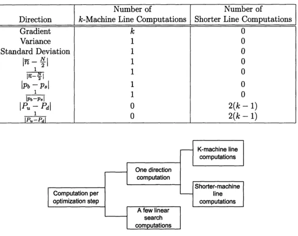
Table 3.1 shows the number of computations needed to calculate the direction for each algorithm. There are two types of direction computations. The first

one is the number of k-machine line computations, which is the number of times

the decomposition algorithm is performed on the k-machine line. The other one is the number of shorter line computations, which is the number of times the decomposition algorithm is performed on part of the k-machine line.

Figure 3-2 shows how the k-machine line computations and the shorter-machine line computations fit into the major computation calculated at each optimiza-tion step.

Table 3.1: Direction Computation Comparisons for the Different Methods Computation per optimization step K-machine line computations Shorter-machine line computations

Figure 3-2: Types of Computations Calculated at Each Optimization Step Next we explain how we obtain the number of direction computations shown in

Table 3.1.

(a) Gradient direction

For the gradient algorithm, the number of computations to calculate the direction is k k-machine line computations.

The gradient is a k - 1-vector. Component i, i = 1, ..., k - 1, indicates the

change in production rate of the line if the capacity of Buffer Bi is increased

by a small amount. In the gradient algorithm, we calculate k-1 production rates associated with the capacity increase of the k -1 buffers. In addition, we also need to calculate the production rate associated with the original

(unmodified) capacity of buffers. Therefore, the total computations needed

Number of Number of

Direction k-Machine Line Computations Shorter Line Computations

Gradient k 0 Variance 1 0 Standard Deviation 1 0 In- N1 ₁ 00 I 1 Pb-p, 1 0 IPb-P 1 O IP - Pdl 0 2(k - 1) IPu-PdI 0 2(k - 1) IP,,-Pdl One direction computation A few linear search computations

to calculate the gradient is k computations.

As the production line gets longer, k gets bigger and the number of

com-putations to calculate the gradient vector gets larger as well.

(b) Variance, standard deviation of buffer Bi's inventory levels, i- , 1 lN,

IPb Ps , iPb-P Directions

In these other algorithms, only one k-machine line computation is

re-quired. With only one decomposition algorithm called, the quantities

fn, Ni,pb(i), s(i), i = 1, ..., k - 1, are calculated simultaneously.

(c) IP, - PdI, PU PdI directions

To calculate IPu(i)- Pd(i) , we hypothetically remove Buffer Bi. There will

be two shorter lines resulting from the removal of Buffer Bi: the shorter line

upstream of Buffer Bi and the shorter line downstream of Bi. To calculate

IP,(i) - Pd(i)l for Buffer Bi, we run the decomposition algorithm twice: first on the upstream portion of the line and the other on the downstream portion. Since there are k - 1 buffers and there are two decomposition algorithms run for each buffer, the number of computations to calculate

P(i) - Pd(i)I or 1 - Vi, i = 1,..., k- 1, is 2(k- 1) shorter line

IPu(i)-Pd (i)

computations.

3.3 Derivation of the New Algorithms

The variance and standard deviation of buffer levels, as well as [n- ¥, Pb -pI,

and I[P - Pdl are indications of buffer level variability and can be used to decide buffer sizes. In Schor's gradient algorithm, the gradient is used to decide how to change buffer sizes. In the new algorithms, the other directions are used to replace the gradient.

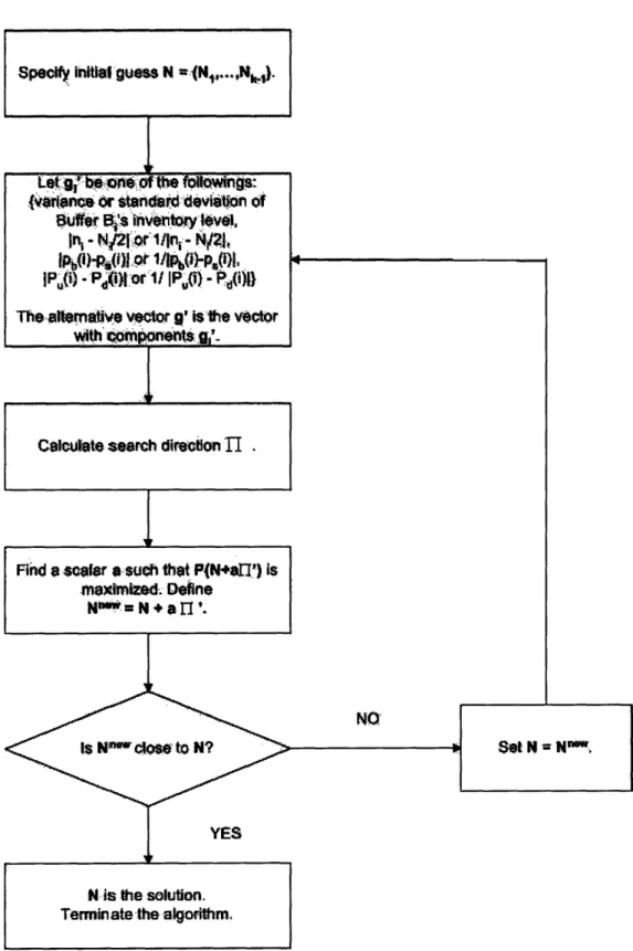
Figure 3-3 shows the block diagram of the new algorithms.

Let vector g' represent any of the alternative directions. In the new algorithms,

Specfy initial guess N -(N,..N.

Find a scar asuch that PN+'aI') is ,mximied Define

N :w=- aN + a ,'.

NO

YES

N, is the solution.

Terrain tethe algorthm.

Figure 3-3: Block Diagram of the New Algorithms

Uat Bdas aa d evit n o.

Uf r sinvntoy level,

h -Ni -1/ or jl -i(qMIPb} l o /1>P9 IP -' P.0d or 1 IP) -P d(i))

Theatemativfe vetor g' is the vctor

WithM w';ponelt

W.<-Calculate search direton II

.1 Set N = L, 11 11111 X -w .- .-- . i "

i

onto the constraint space. The projected vector is called

fI'.

Chapter 4

Performance of the New

Algorithms

The performance of the new algorithms will be evaluated in terms of:

1. Accuracy

Accuracy measures how close the final production rates of the new algorithms to the final production rate of the gradient.

2. Reliability

Reliability measures how often the final production rates of the new algorithms converge to the final production rate of the gradient algorithm.

3. Speed

Speed measures how fast the new algorithms converge.

4.1 Accuracy

We access the accuracy of the new algorithms by studying the effects of the followings:

1. Identical versus non-identical machines

Let final P be the production rate when each algorithm terminates. Two-machine

line counter is defined as the number of times we evaluate the hypothetical

two-machine line in the decomposition algorithm. The two-two-machine line counter is counted at each optimization step. Final two-machine line counter is the two-machine line

counter when each algorithm terminates. The final two-machine line counter is used

to measure the speed of each algorithm.

We compare the performance of all algorithms by comparing their final production rates and their final two-machine-line counters.

4.1.1 Identical versus Non-Identical Lines

Identical Machines

To study the impact of the identicmachine line on the performance of the new al-gorithms, we randomly generated 15 lines using the procedure described in Appendix

A. The length of the line generated ranges from 8 machines to 36 machines. Figure

4-1 shows the average, the maximum, and the minimum of the proportion of the final production rates of the other algorithms to the final production rate of the gradient algorithm. Figure 4-2 shows the average, the maximum, and the minimum of the proportion of the final two-machine-line counters of the other algorithms to the final two-machine-line counter of the gradient algorithm.

I I

XA- ~_

Figure 4-1

i

Figure 4-1: Final P of the Other Directions as Proportions of Final P of the Gradient in the Identical Machine Case

l Average | I Maximum Minimum 2 m E X . ;t .e Ci ! 10 1 5

e~~~~~~P~~~~ 4 U~~~il Average 3. 5 n Maximumn Minimum 0e 3 2.5 6~ 1.5 E 1

lu

I

1H-f

t

.a

r

-

o

Figure 4-2: Final Two-Machine Line Counter of the Other Directions as Proportions

of Final Two-Machine Line Counter of the Gradient in the Identical Machine Case

Figure 4-1 and Figure 4-2 show that the variance and the standard deviation work very well as substitutes for the gradient. This is because the final P of the variance and standard deviation algorithms are as high as the final P of the gradient algorithm and the convergence times of the two algorithms are, on average, half that of the gradient algorithm. We do not recommend using 1 and I to

ra-

-'

replace gi (component i of the gradient) because their convergence times might be as long as four times the convergence times of the gradient algorithm. The other directions (1P-PI' ¥, - Pb- p81, and IP,, - Pda) do not outperform the gradient

because their final production rates are slightly lower than the final production rate of the gradient. Although their average convergence times are lower than that of the gradient, occasionally their convergence times might be longer than the convergence time of the gradient.

Figure 4-3 shows that the P and the two-machine-line counter at each optimization

step for one of the line generated. The parameters of the line are described in Table

4.1. The variance and standard deviation algorithms reach the final P of the gradient algorithm in only a few steps. On the other hand, the gradient algorithm takes longer to achieve and exceed the final P of the variance and the standard deviation algorithms.

Table 4.1: The Line Parameters of which Results are Shown in Figure 4-3 101.2 101 -R0 .2 0 -0 2 100.8 100.6 100.4 100.2 100 0 1000000 2000000 3000000 4000000 5000000 6000000

Two Machine Line Counter

Figure 4-3: Production Rate versus Two-Machine Line Counter for an Identical Ma-chine Case

Non-Identical Machines

We also study the impact of non-identical machine lines on the performance of the new algorithms. Nineteen lines that consist of non-identical machines are generated

according to the procedure described in Appendix A. The line length generated ranges from 7 to 40 machine line and might contain up to three bottlenecks. The selection and severity of the bottlenecks are randomly generated according to the procedure in

Appendix A.

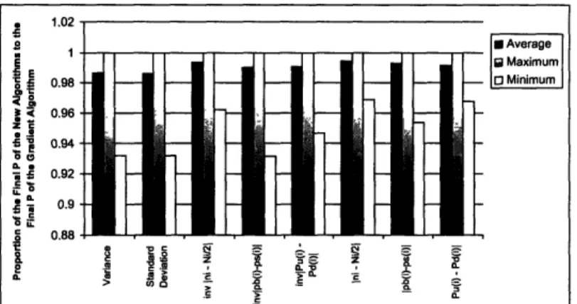
Figure 4-4 shows the average, the maximum, and the minimum of the proportion of the final P of the other algorithms to the final P of the gradient algorithm. Figure 4-5 shows the average, the maximum, and the minimum of the proportion of the final two-machine-line counter of the other algorithms to the final two-machine-line counter of the gradient algorithm.

Number of Machines 30 identical machines

Total Buffer Space to be Allocated 745

Repair Rate r 7.096 Failure Rate p 0.874 Processing Rate p/ 141.531

I.U .9 1 E cE 0.98 . ° 0.96 0 0.94 0.92 jE 0.92 s ,g 0.88 aL 5 0.86 · Average Maximum [ Minimum o o . t C. .- G3.~~ , = z [ t.-- ., ' ,

Figure 4-4: Final P of the Other Directions as Proportions of Final P of the Gradient in the Non-Identical Machine Case

Figure 4-4 and Figure 4-5 show that the variance and the standard deviation

algorithms also do well in the non-identical machine case, although not as well as in

the identical machine case. This is shown by the fact that the average final P of the

two algorithms are 0.984 of the average final P of the gradient algorithm (compared with an average of .999 in the identical-machine case) and the average convergence

times are less than half the convergence time of the gradient algorithm. We do not recommend using l P()(i)

_{IP~(W)-Pd(i)I}

_{2 - -}

greatly. For example, the final two-machine line counter of the IP1 direction can be as small as 0.05 the final two-machine line counter of the gradient, but can be as

big as 40 times that of the gradient.

4.1.2

The Location, Existence, and Severity of Bottlenecks

Existence of Bottleneck in Short and Long Lines

In this section, we investigate the performance of the new algorithms in the following

cases:

* Short lines with bottlenecks

* -n

Figure 4-5: Final Two-Machine Line Counter of the Other Directions as Proportions of Final Two-Machine Line Counter of the Gradient in the Non-Identical Machine

Case

* Short lines with no bottlenecks * Long lines with bottlenecks

* Long lines with no bottlenecks

Short lines are defined as lines with less than 30 machines and long lines as lines

with more than 30 machines. Lines with bottlenecks can contain up to three bot-tlenecks, with Pbottleneck between 0.5 and 0.8 of the minimum p of the other

non-bottlenecks.

To minimize the effects of outside factors (factors other than short lines versus long

lines and lines with bottlenecks versus lines without bottlenecks) that influence the performance of the new algorithms, the short lines with bottleneck are created from the short lines with no bottleneck by converting a randomly chosen non-bottleneck

into a bottleneck. This is done by imposing a low isolated machine production rate p on the bottleneck. Similarly, long lines with bottleneck are created from long lines without bottleneck by converting a previously non-bottleneck by imposing a low p on

it. We created 10 short lines with bottlenecks and 10 short lines without bottlenecks. The results for short lines with bottleneck are shown in Figure 4-6 and Figure 4-7. The results for short lines without bottleneck are shown in Figure 4-8 and Figure 4-9.

I I.. 1

Figure 4-6: Final P of the Other Directions as Proportions of Final P of the Gradient Algorithm in Short Lines with Bottlenecks

Figure 4-7: Final Two-Machine Line Counter of the Other Directions as Proportions of Final Two-Machine Line Counter of the Gradient Algorithm in Short Lines with Bottlenecks

Figure 4-6, Figure 4-7, Figure 4-8, and Figure 4-9 show that the new algorithms perform better in lines with no bottlenecks than in lines with bottlenecks. This is because in lines with no bottlenecks the final P of the new algorithms are in the neighborhood of the final P of the gradient algorithm and the final two-machine line counter of the new algorithms are smaller than that of the gradient algorithm. The results that the new algorithms perform better in non-bottleneck cases are even more apparent in longer lines as shown in Figure 4-10, Figure 4-11, Figure 4-12, and Figure

4-13. Figure 4-12 shows that the final P of the new algorithms are very close or

' 1.UZ 1 0.98

og4

Figure 4-8: Final P of the Other Directions as Proportions of Final P of the Gradient Algorithm in Short Lines with No Bottlenecks

higher than the final P of the gradient algorithm. Figure 4-13 demonstrates that, on average, the new algorithms converge much faster than the gradient algorithm.

Location and Severity of Bottlenecks

We also study the effects of locations of a bottleneck and severity of a bottleneck on the performance of the new algorithms. We first create lines with no bottlenecks. From

these lines with no bottlenecks, we create lines with a bottleneck on the upstream, lines with a bottleneck on the middle stream, and another lines with a bottleneck on the downstream. The parameters of the non-bottleneck machines in lines with bottleneck are the same as the parameters of the non-bottleneck machines in the

original lines with no bottleneck. The bottleneck is created by imposing a low p on a randomly chosen machine. To minimize the effects of outside factors, the parameters

of the bottleneck located upstream, middle stream, and downstream of the lines are

the same. At first, these bottlenecks are made less severe, with p of the bottleneck is

between 0.8 and 0.95 of the minimum p of the other machines. Later, the bottlenecks

are made more severe, with p of each bottleneck is < 0.8 of the minimum p of the other machines. As before, we first study the effects on identical machine lines and later on the non-identical machine lines. In the identical machine case, all machines, except the bottleneck, are identical. In the non-identical machine case, all machine

54 1.UU5 o a 1 E 0.995 = <

0.99

Figure 4-9: Final Two-Machine Line Counter of the Other Directions as Proportions of Final Two-Machine Line Counter of the Gradient Algorithm in Short Lines with

No Bottlenecks

Figure 4-10: Final P of the Other Directions as Proportions of Final P of Algorithm in Long Lines with Bottlenecks

the Gradient are different with the bottleneck having the lowest p of all.

In both the identical and non-identical machine cases, the location of bottlenecks

does not strongly affect the final P of the new algorithms, as shown in Figure 4-14,

Figure 4-15, and Figure 4-16 for the identical machine case. These figures show that the proportion of the final P of all the algorithms to the final P of the gradient algorithm are similar, regardless of the location of the bottleneck. The speeds of the new algorithms, except the variance and the standard deviation algorithms, are slightly affected by the location of the bottleneck, as shown in Figure 4-17, Figure

1.02 E 1 C Average I E D Maximum 0.98

i- I

H H

.H

H

'

1 I

F I Minimum

|

Average I

_C Maximum

Minimum

Figure 4-11: Final Two-Machine Line Counter of the Other Directions as Proportions

of Final Two-Machine Line Counter of the Gradient Algorithm in Long Lines with

Bottlenecks I A I.LP~ 1.02 Z 0.98 0.96 *. 0.94 . 0.92 I'

22K

Figure 4-12: Final P of the Other Directions as

Algorithm in Long Lines with No Bottlenecks

Proportions of Final P of the Gradient 4-18, and Figure 4-19. For example, Figure 4-17 shows that it takes at most 9 times the speed of the gradient algorithm for the _IPb-PsI1 algorithm to converge when the bottleneck is located upstream in the identical machine line. However, Figure 4-18 demonstrates that it takes at most only 2.5 times the speed of the gradient algorithm for the 1P algorithm to converge when the bottleneck is located in the middle of

the line. Unfortunately, we could not explain how the speed of the new algorithms vary with the locations of the bottleneck. As mentioned earlier, the speed of the variance and standard deviation algorithms is not affected by the location of the