Publisher’s version / Version de l'éditeur:
Cold Regions Science and Technology, 3, pp. 237-242, 1980
READ THESE TERMS AND CONDITIONS CAREFULLY BEFORE USING THIS WEBSITE. https://nrc-publications.canada.ca/eng/copyright
Vous avez des questions? Nous pouvons vous aider. Pour communiquer directement avec un auteur, consultez la première page de la revue dans laquelle son article a été publié afin de trouver ses coordonnées. Si vous n’arrivez pas à les repérer, communiquez avec nous à [email protected].
Questions? Contact the NRC Publications Archive team at
[email protected]. If you wish to email the authors directly, please see the first page of the publication for their contact information.
NRC Publications Archive
Archives des publications du CNRC
This publication could be one of several versions: author’s original, accepted manuscript or the publisher’s version. / La version de cette publication peut être l’une des suivantes : la version prépublication de l’auteur, la version acceptée du manuscrit ou la version de l’éditeur.
Access and use of this website and the material on it are subject to the Terms and Conditions set forth at
Three-time-level methods for the numerical solution of soil freezing
problems
Goodrich, L. E.
https://publications-cnrc.canada.ca/fra/droits
L’accès à ce site Web et l’utilisation de son contenu sont assujettis aux conditions présentées dans le site
LISEZ CES CONDITIONS ATTENTIVEMENT AVANT D’UTILISER CE SITE WEB.
NRC Publications Record / Notice d'Archives des publications de CNRC:
https://nrc-publications.canada.ca/eng/view/object/?id=34d3ad22-2cd6-4077-aadb-742e06120c71 https://publications-cnrc.canada.ca/fra/voir/objet/?id=34d3ad22-2cd6-4077-aadb-742e06120c71Ser
TH1
National Research
Conseil national
N21d
Coundl Canada
ds
recherches Canada
THREETIMELEVEL METHODS FOR THE
NUMERICAL SOLUTION OF SO
Reprinted
from
Cold
Regions Science and Technology
Vol. 3,
1980p. 237
242
DBR
Paper No.
925
Division of Building Research
Price
$1.00
OTTAWA
NG PROBLEMS
NRC-
CISTIBLDG.
RES.
L I B R A R Y
81-
09-
0
7
e l z k l
3 r 9 . s : ; ~ ; l ~
% * <: 7. 1-
.C-
lClSTr
LSO MMAIRE
L e s methodes p a r Clement fini e t p a r difference finie utilisCes pour rCsoudre l e s problkmes de t r a n s f e r t de chaleur et de m a s s e t r a i t e n t habituellement l a d e - rivCe par rapport au temps e n s e basant s u r d e s calculs e n d e w points du temps. Dans l e s probl'emes de gel et de dkgel, les dquations sont non linkaires. L1absence de linCarit6 e s t due 'a l a ddpendance des propri6tCs du materiau s u r l a temp6rature e t 11humidit6. Avec l a mCthode des calculs e n deux points du t e m p s , i l faut habituellement proceder p a r itbration, afin dlobtenir des r e s u l t a t s prbcis.
P o u r l e s situations non l i n e a i r e s de ce type, on peut s l e x e m p t e r du p r o c e s s u s d l i t e r a t i o n en utilisant un calcul en t r o i s points du temps, dans lequel on 6value l e s propriCtCs du materiau au point intermediaire. Le calcul le plus connu de ce type e s t cependant sujet 'a
oscillation, ce qui r e s t r e i n t grandement son utilitC. - Le p r e s e n t document t r a i t e dlune nouvelle m3thode de calcul e n t r o i s points du temps e t la compare, e n ce qui a t r a i t 'a l a precision e t 'a l a susceptibilit6 'a 1'0s- cillation, avec plusieurs a u t r e s mdthodes de calculs basdes s u r la variation reguli'ere par rapport au temps.
Cold Regions Science and Technology, 3 (1980) 237-242
O Elsevier Scientific Publishing Company, Amsterdam - Printed in The Netherlands
THREE-TIME-LEVEL METHODS FOR THE NUMERICAL SOLUTION OF SOIL FREEZING PROBLEMS
L.E. Goodrich
Geotechnical Section, Division of Building Research, National Research Council of Canada
I (Ottawa)
ABSTRACT where (81 is the vector of nodal
Finite element and finite difference methods temperatures, {8} represents time derivatives for heat and mass transfer problems are and the thermal capacitance, and conductance usually based on two-time-level schemes for matrices [C] and [K] are temperature
treating the time derivative. In freezing dependent. The most widely used time- and thawing problems the equations are non- stepping procedure is the Crank-Nicholson linear. The non-linearity arises because of central time difference scheme:
the dependence of the material properties on At m+l
both temperature and moisture fields. With
[c]
i e ~ ~ + l -[cl
{elm
+ [K] (61two-time-level schemes it is usually At m
+ [K]
{el
= 0necessary to iterate the solution in order to obtain accurate results.
For non-linear problems of this type iteration can be avoided by using a three- time-level scheme with material properties evaluated at the intermediate time level. The most well known three-time-level scheme is, however, subject to oscillation which seriously limits its usefulness.
This paper discusses a new three-time- level scheme and compares it with several other time marching schemes from the stand- point of accuracy and susceptibility to oscillation.
For non-linear heat flow problems such as occur in freezing and thawing soils, spatial discretization using either finite elements or finite differences leads to the system of equations
[C] + [K] = 0 (1)
While the simplest procedure to accommodate temperature-dependent thermal properties is to update the coefficient matrices at the beginning of each time step using the known thermal properties from the old time level, to ensure accuracy and convergence it is preferable to use values [c]'"+~/~ and
[K] m+1/2, determined at an intermediate time level. Because the thermal properties are functions of the unknown temperatures, {81~+', iteration is required for solution. It is generally conceded that, for one- and two-dimensional linear heat flow problems, direct solution techniques are more
efficient.
Direct solution methods can be retained for non-linear problems by using a three- time-level formulation in which the thermal properties are evaluated at the intermediate time level. A well known three-time-level scheme (Douglas 1961) consists in replacing the time derivative in eqn. (1) by a
temperature vector is replaced by a simple average of values at three-time levels, viz.,
2At [C] - [C]
{elm-'
+ [K]({elm+'
+{elm
+ie~~-')
=o
(3)This method has been used with finite difference schemes by Bonacina and Comini
(1973) and Bonacina et a1 (1973). A finite element formulation for heat transfer with phase change is described in Comini et a1
(1974). Although eqn. (3) is unconditionally stable, the method is subject to serious oscillations. Comini and Lewis (1976) describe an averaging procedure that is helpful in controlling the oscillation but that does not eliminate it.
A general method of formulating multi-time level marching methods using finite elements in time is outlined in Zienkiewicz (1971). Assuming an interpolated form for the time- dependent temperature vector
j =m-n
where ~ e l j is the nodal temperature vector at time level j, and N j (t) are shape functions in time, then applying the Galerkin weighted residual procedure to eqn. (1) gives
Only one weighted residual equation is required because the temperatures are known at time levels j (m.
Using quadratic Lagrange polynomials as shape functions leads to a three-time-level formulation. In terms of the local time
T = t
-
tm-l, the element shape functions arewhere A = tm - tm-'
1 , and = tm*' - tm. Combining eqns. (4), (5) and (6) and assuming that [C] and [K] are independent of time in the interval tm-I - - < t < tm+l, yields
[cl
[(a-a){elm-l
-
+slelrn+']
b
A1+A2 + - .
10 [K] ((10-3a){01~'~ + (3-26)a
.
{elrn
where 6 = A1/A2, and a = (1+6)
.
(1+1/6). For a fixed time step A1 = A = At,2 eqn. (7) reduces to
( - { 8 1 ~ - ~ + 2(01rn + 4(81~+'] = 0 (8)
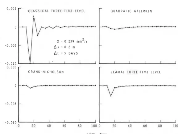
Figure 1 illustrates the behaviour of the truncation error of the quadratic Galerkin three-time-level scheme, eqn. (8), compared with that for several other schemes. The problem considered is that of one-dimensional heat conduction in an homogeneous semi- infinite medium initially isothermal at zero temperature and whose surface is suddenly brought to temperature -1. The grid spacing, time step and thermal diffusivity values assumed are indicated on the figure and correspond to a ~ t / A x ~ = 2.58. In all cases the numerical solution was started at time level 3At using the analytical solution to generate temperature values at time levels At, 2At. The figure shows the over-all error for the first interior node point.
As seen in Fig. l(a), the method of eqn. (3) results in very large oscillations. Although stable, oscillation of this
magnitude could lead to serious errors in problems with time dependent boundary conditions or with temperature dependent
C L A S S I C A L T H R E E - T I M E - L E V F L
m-*t
/*,=.\...*.-.C.-.-.-.-.-.-.
2 a = 0 . 2 3 9 m m I s A X = 0 . 2 m A t = 5 D A Y S I I . I t I-
C R A N K - N I C H O L S O N--.
'.#
.LL.C.-.-.-.-.-.-.-.-.-.-.-.-.-.-
I I I I I T I M E , d a y sFig. 1. Truncation error for a simple heat flow problem.
thermal properties. The quadratic Galerkin give more accurate over-all results than
scheme, eqn. (8), gives results shown in Z15malfs scheme when applied to practical
Fig. l(b) similar to those of the Crank- problems with temperature dependent thermal
Nicholson scheme, Fig. l(c). The quadratic properties.
-
Q U A D R A T I C G A L E R K I N-
.-.\
-*C.C.-.d-.-
-t.-.-..-.--.-.-.-.--
I I I I I-
Z L A M A L T H R E E - T I M E - L E V E L-
.-.
,-,_.-*-.-.-.-.-.-.-.-.-a-.-.-.
\/-
-
I I I I IGalerkin method does, however, exhibit slightly greater errors than those of eqn. (2) during the first few time steps. Results for a three-time-level scheme proposed by Zl5mal (1975) are shown in
Fig. l(d). Although the error of Z15ma11s
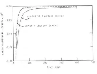
In order to verify the performance of the quadratic Galerkin scheme with variable time steps, eqn. (7) was applied to the sample problem of Fig. 1, using a ratio of succes- sive time steps Atrn+l/~trn = 1.1. This
scheme is slightly superior to that of the corresponded to an increase in the parameter
quadratic Galerkin scheme for intermediate aAt/ax2 from 2.58 to 21.0 after 24 time
times, relatively larger errors occur at steps. The results, shown in Fig. 2,
early times with Z15ma11s method. Both indicate that the quadratic Galerkin variable
Z15malfs scheme and the quadratic Galerkin time step scheme is satisfactory. The
truncation error is, however, somewhat larger scheme are distinctly superior to the three-
than that of the Crank-Nicholson scheme.
time-level scheme of eqn. (3). Because the
quadratic Galerkin scheme produces a more Z15malfs scheme is obtained from the
Fig. 2. Truncation error with increasing time step.
with coefficients a. f3. chosen so as to
J J
minimize the maximum modulus of the roots of the characteristic equation. In this way the stability of the scheme for large time steps should be improved.
In terms of the Zienkiewicz two-parameter three-time-level scheme described in
Wood (1978)
Z15malts scheme corresponds to a = $ + a
B = kj(1 + u) 2 (11)
O < U L l
which, with u = 1/3 as recommended by ZlBmal, gives,
a = 5/6
B = 4/9 (12)
By inspection, eqn. (8) also corresponds
to eqn. (10) but with a = 3/2
B = 4/5
In the notation of Wood (1978), eqn. (10) is A. stable if a 2 % and B > 4 2 . The method is second order with error coefficient
C = -1(1/12 + f3 - a/2) (14) Thus the quadratic Galerkin scheme, eqn. ( 8 ) , is A stable but the error coefficient is
0
c
= -(1/12 + 1/20)while for Z15ma17s scheme, with a = 1/3, C = -(1/12 + 1/36)
Woods (1978) compared the behaviour of several multi-level schemes for the pure initial value problem
- dy - - - y ; y(0) = 1
dt (15)
and concluded that Zlgmal's scheme was subject to unacceptable oscillation at large values of step length. Wood's numerical experiments were repeated and the results are summarized in Table 1. Table l(a) for step length At = 0.5 shows ZIBmalfs scheme to be inferior to the quadratic Galerkin scheme for the first three steps. The superior
truncation error of Zlgmal's scheme does, however, show up at subsequent steps. Table l(b) shows the results when the step length is increased to At = 5.0. In this case the quadratic Galerkin scheme produces results with a distinctly smaller oscillation than that of Z15malfs scheme. As a result, the over-all error is also considerably better for the quadratic Galerkin scheme.
Table 1 also contains results calculated using the "classical" three-time-level method
(eqn. (3)) with smoothing as recommended by Comini and Lewis (1976). Although smoothing is helpful for At = 0.5, for At = 5.0 the truncation error and oscillation are nearly as bad with as without smoothing. In all
241
TABLE 1 (a)
Comparison of errors for various one- and two-step methods At = 0.5
Exact Error (Numerical
-
Exact) for 1-step methods t-t Backward Crank- Linear
y=e Difference Nicholson Galerkin
1 .O 3.679E-01 3.647E-02 -3.961E-03 1.120E-02
' 1.5 2.231E-01 4.644E-02 -4.779E-03 1.380E-02 2.0 1.353E-01 4.438E-02 -4.325E-03 1.274E-02 2.5 8.208E-02 3.772E-02 -3.479E-03 1.046E-02
.
3.0 4.979E-02 3.009E-02 -2.623E-03 8.056E-03 3.5 3.02OE-02 2.305E-02 -1.899E-03 5.955E-03 4.0 1.832E-02 1.718E-02 -1.337E-03 4.279E-03 4.5 1.lllE-02 1.256E-02 -9.216E-04 3.013E-03 5.0 6.7388-03 9.039E-03 -6.255E-04 2.088E-03Exact Error (Numerical - Exact) for 2-step methods t
-t Comini and Quadratic
y=e Classical Lewis Zldmal Galerkin
1.0 3.679E-01 -1.951E-02 -1.9518-02 -7.235E-03 -3.799E-03 1.5 2.2318-01 -6.957E-03 1.559E-02 -7.435E-03 -5.901E-03 2.0 1.353E-01 -1.519E-02 1.144E-02 -6.553E-03 -6.188E-03 2.5 8.208E-02 -4.033E-03 1.429E-02 -5.156E-03 -5.468E-03 3.0 4.979E-02 -9.230E-03 1.100E-02 -3.840E-03 -4.391E-03 3.5 3.020E-02 -1.311E-03 9.093E-03 -2.754E-03 -3.321E-03 4.0 1.832E-02 -5.259E-03 6.704E-03 -1.924E-03 -2.410E-03 4.5 l.lllE-02 7.002E-05 4.968E-03 -1.318E-03 -1.699E-03 5.0 6.738E-03 -3.004E-03 3.536E-03 -8.901E-04 -1.172E-03
TACLE 1 (b)
Comparison of errors for various one- and two-step methods At = 5.0
Error (Numerical
-
Exact) for 1-step methodst Exact
Backward Crank- Linear
-t
v=e Difference Nicholson Galerkin
Exact Error (Numerical
-
Exact) for 2-step methodsComini and Quadratic
cases the method remains distinctly inferior to both Z15ma17s and the quadratic Galerkin scheme.
CONCLUSION
The quadratic Galerkin three-time-level scheme presented here is distinctly superior to the usual three-time-level scheme as regards to both oscillation and truncation error. Although the truncation error is slightly greater than that for a similar method proposed by Zldmal, the quadratic
Galerkin method remains usable over a larger range of step lengths and, for this reason, should be more attractive for practical applications.
REFERENCES
Bonacina, C. and Comini, G. (1973), On the solution of the nonlinear heat conduction equations by numerical methods, Int. J. Heat Mass Transfer, 16: 581-589.
Bonacina, C., Comini, G., Fasano, A. and Primicerio, M. (1973), Numerical solution of phase-change problems, Int. J. Heat Mass Transfer, 16: 1825-1832.
Comini, G., Del Guidice, S., Lewis, R.W., and Zienkiewicz, O.C. (1974), Finite element solution of non-linear heat conduction problems with special reference to phase change, Int. J. Num. Meth. Eng., 8: 613-624. Comini, G. and Lewis, R.W. (1976),
A numerical solution of two-dimensional problems involving heat and mass transfer,
Int. J. Heat Mass Transfer, 19: 1387-1392. Douglas J. (1961), A survey of numerical methods for parabolic differential equations in Advances in Computers, Academic Press,
-
New York, Vol. 2, pp. 1-54.
Wood, W.L. (1978), On the Zienkiewicz three- and four-time-level schemes applied to the numerical integration of parabolic equations,
Int. J. Num. Meth. Eng., 12: 1717-1726. Zienkiewicz, O.C. (1971), The finite element in engineering science, McGraw-Hill, London, 521 p.
Zldmal, M. (1975), Finite element methods in heat conduction problems, Proc. Conf. Finite Element Methods, Brunel University, pp. 85-104.
This publication is being d i s t r i b u t e d by the Division of Building R e s e a r c h of the National R e s e a r c h Council of Canada. I t should not be reproduced in whole o r in p a r t without p e r m i e s i o n of the original publisher. The Di- vision would b e glad to b e of a s s i s t a n c e in obtaining s u c h permiseion.
Publications of the Division m a y b e obtained by m a i l - ing the a p p r o p r i a t e r e m i t t a n c e ( a Bank, E x p r e s s , o r P o s t Office Money O r d e r , o r a cheque, m a d e payable t o the R e c e i v e r G e n e r a l of Canada, c r e d i t NRC) t o the National R e s e a r c h Council of Canada, Ottawa. K1A O R 6 .
Stamps a r e not acceptable.
A l i s t of a l l publications of the Division is available and m a y be obtained f r o m the Publications Section, Division of Building R e s e a r c h , National R e s e a r c h Council of Canada, Ottawa. KIA OR6.