HAL Id: hal-01096829
https://hal-brgm.archives-ouvertes.fr/hal-01096829
Submitted on 18 Dec 2014
HAL is a multi-disciplinary open access
archive for the deposit and dissemination of
sci-entific research documents, whether they are
pub-lished or not. The documents may come from
teaching and research institutions in France or
abroad, or from public or private research centers.
L’archive ouverte pluridisciplinaire HAL, est
destinée au dépôt et à la diffusion de documents
scientifiques de niveau recherche, publiés ou non,
émanant des établissements d’enseignement et de
recherche français ou étrangers, des laboratoires
publics ou privés.
Innovative Methodology to Compute the Temperature
Evolution of Pile Heat Exchangers
Charles Maragna, Xavier Rachez
To cite this version:
Charles Maragna, Xavier Rachez. Innovative Methodology to Compute the Temperature Evolution
of Pile Heat Exchangers. World Geothermal Congress 2015, Apr 2015, Merlbourne, Australia.
�hal-01096829�
Melbourne, Australia, 19-25 April 2015
Innovative Methodology to Compute the Temperature Evolution of Pile Heat Exchangers
Charles Maragna and Xavier Rachez
BRGM, 3 Avenue Claude-Guillemin, BP 36009 – 45060 Orléans cedex 2 – France [email protected]
Keywords: closed-loop heat exchangers, pile heat exchangers ABSTRACT
Energy geostructures such as heat exchanger piles couple the structural role of geostructures with heat and cold supply via shallow geothermal energy. This combination makes it possible to cut down the investment costs of ground heat exchangers (GHE). Thermal dynamic simulations require numerical models of pile heat exchangers to run over a reasonable amount of time. In this perspective semi-analytical models seem interesting. The paper presents an approach to semi-analytical modeling of pile heat exchangers. This approach relies on three elements: First, correlations are established to describe the evolution of wall pipe temperature under constant heat load in presence of underground water flow. These correlations take into account the underground water flow in the vicinity of the pile, allowing the computation of the temperature evolution over both the short and long terms. Second, a resistive-capacitive (RC) circuit is developed to account for the thermal inertia of the pile concrete without having to mesh its geometry. Third, the RC circuit is combined to a heat balance over the heat carrier fluid and to correlations to compute temperature evolution in the fluid. Predictions of this semi-analytical model are compared with those of a fully-discretized finite elements model. A good agreement between both models is reached. Acquisition of in-situ data is foreseen to validate both models.
1. INTRODUCTION
Geothermal energy is becoming widely used to supply buildings with renewable heating and cooling. This development has been taking place in a context of policies fostering the reduction of green-houses gas emission. For instance the total number of geothermal heat pumps installed in Europe has been recently estimated to reach 1,140,000 and to represent an equivalent thermal power of 14,000 MWth (Observ‟ER, 2013). In this context, a diversification of the heat sources and sinks of ground-sourced heat pumps has been researched. Energy geostructures such as piles heat exchanger (Figure 1) appear to be an attractive technology as costs for both geostructures and ground heat exchanger (GHE) realization are mutualized which allows cutting down the costs of GHE achievement. The dual role of the energy geostructures (mechanical and energetics) makes their design more complex and challenging (Laloui and Di Donna, 2013).
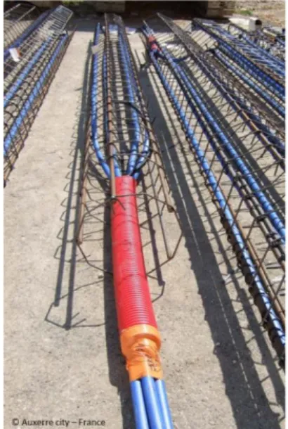
Figure 1: Example of a pile heat exchanger (PHE) before installation in ground (with the courtesy of Auxerre city – France)
The thermo-mechanical behaviour of energy geostructures has been and is still extensively studied (Suryatriyastuti et al., 2012, Di Donna, 2014), and helps developing thermo-mechanical design tools of energy piles. The thermal performance of energy piles has been less studied in details and still needs improvement. For instance, the energy pile thermal design may be inadequate if the same design approaches as for borehole heat exchangers is used for piles (Bourne-Webb, 2013).
A thermal dynamic simulation is often necessary to optimize the energetic system made of ground heat exchangers, heat pump and building. To do so it appears mandatory to rely on numerical models of pile heat exchangers (PHE) that run over a reasonable amount of time. The resolution of the heat and mass balance equations with numerical techniques such as the finite element (FE) often leads to computation times that are not compatible with engineering practices. Analytical solutions are an alternative.
However the range of these solutions is often limited due to the fact that no known analytical solution describes both the cylindrical GHE geometry and the surrounding underground water flow correctly (Wagner et al., 2013).
The paper presents a new approach to semi-analytical thermal modeling of pile heat exchangers. This approach relies on three innovative elements. After a short presentation of assumption (section 2.1.), the paper first presents correlations that have been established over the temperature evolution of the wall pipe under constant heat load, referred to as step response (section 2.2). These step responses have been designed to correctly describe the temperature evolution in the vicinity of the pile. Second, a resistive-capacitive (RC) circuit is developed to account for the thermal inertia of the pile concrete (section 2.3). Third, the RC circuit is combined to a heat balance over the heat carrier fluid and to correlations for step response to obtain a semi-analytical model. A numerical scheme is used to solve temperatures in the fluid, pile and surrounding ground: Temperatures at the nodes of the RC circuit and in fluid are solved with an implicit Euler method, while the evolution of pile wall temperature is computed by discretizing the convolution of time-variable heat flux with the step response (section 2.4). Finally, predictions of the semi-analytical model model are compared with those of a fully-discretized finite elements model (section 3).
2. DESCRIPTION OF THE INNOVATIVE METHODOLOGY 2.1. Assumptions
Throughout the whole paper, the following assumptions are made:
(i) The ground is regarded as a homogenous porous media saturated with water where Darcy‟s law applies.
(ii) At the scale of observation, the concrete material properties are supposed to be homogeneous. As the hydraulic conductivity of concrete for piles would typically be of the order of 10-12 m/s, the concrete is considered as an impermeable material.
(iii) Strains originating from thermal stresses are not taken into account in this paper. Both pile concrete and soil matrix are therefore considered to be non-deformable.
(iv) Physical properties of the materials (underground water, soil matrix, PHE heat carrier fluid) do not depend upon temperature.
(v) The initial, non-disturbed temperature T0 is constant in the whole domain; far away from the pile heat exchanger
temperature remains constant. In what follows we simply set T0=0 K.
(vi) Underground water flows and heat transfer occurs in a horizontal plan. Underground water flow is determined in stationary regime.
2.2 Moving infinite cylindrical source model. New approach
This section aims at developing a “step response” function that describes the temperature evolution at the pile wall under a constant linear heat flux (i.e. per borehole length unit, in W.m-1
) in presence of underground water flow (cf. Figure 2):
(1)
denotes the thermal conductivity of the porous media (W.K-1.m-1). accounts for moving infinite cylindrical source model.
Figure 2: Scheme of the modeled domain and boundary condition
Water flow in the soil matrix is driven by hydraulic head gradient, according to Darcy‟s law:
(2)
Where denotes the Darcy velocity (m.s-1), the hydraulic conductivity (m.s-1), the hydraulic head (m). Under the assumption
of incompressible water, the equation for water mass conservation reads:
( ) (3)
Heat in a homogenous porous medium with ground water flow is transported by conduction and advection. The partial derivative equation for energy conservation reads:
( ) ( ) (4) Where the subscripts and respectively denote the ground and the underground water. The volume-specific heat capacity ( ) (J.K.m-3) of the porous media is related to the volume-specific heat capacities of the matrix ( ) and of the water ( ) by:
( ) ( ) ( ) (5)
refers to the total porosity of the porous media.
As the set of partial derivative equations (3) and (4) are linear, they can be normalized. Two dimensionless numbers, Fourier Fo and Peclet Pe, are introduced. We took as reference length the radius of the pile . Hence a normalized length of is:
(6)
Fo is the Fourier number characterizing the ratio of diffused heat to stored heat:
(7)
is a normalized time. This involves that in dynamic simulation Fo replaces the time t. is the thermal diffusivity of the ground (m².s-1) defined by:
( ) (8)
The Peclet number is a parameter accounting for the ratio of the heat transferred by convection to the heat transferred by conduction:
( ) (9)
Higher Peclet numbers lead to non-negligible convection compared to conduction. denotes the “undisturbed” Darcy flow, i.e. far away from the pile, where the impermeable pile doesn‟t deflect underground water flow.
The normalized equation for heat transport reads:
(10)
Normalizing the heat equation has a huge advantage: It makes it possible to greatly decrease the number of parameters involved in the problem. The temperature T at a point of coordinates (x, y) depends on five parameters (( ) , , ( ) , , ) and three variables (x, y, t) while the normalized temperature T* depends on a single parameter (Pe) and three variables (x*, y*, Fo). The step response is the normalized temperature averaged on the pile wall perimeter . Therefore, depends on one parameter (Pe) and one variable (Fo) :
∫ (11)
For practical engineering problems, the temperature evolution at the pile wall can be computed based if the step response is known thanks to Equation (1).
Carslaw and Jaeger (Carslaw and Jaeger, 1947) analytically determined a step response in case heat is only transferred by conduction (no convection, i.e. Pe=0) where the cylindrical geometry of the borehole is accounted for. This step response GICS is
referred to as the infinite cylindrical source (ICS) model:
∫ ( ) (12)
Here refers to the classical function evaluated at the pile wall, i.e. for the normalized distance from the pile axis . The same authors provided another step response where conduction and convection are taken into account, but where the pile cross-section degenerates to a point. This step response is here denoted GMILS and is known as the moving infinite line source
(MILS) model. It can be expressed as a function of Fo and Pe as:
( ) ( ( ) ) (13)
The MILS model replaces the cylindrical geometry of the pile by a simple line. Therefore, it does not correctly account for the cylindrical geometry of the pile. Consequently the temperature evolution on short duration is not described well. Moreover, Wagner et al. (Wagner et al., 2013) reported that using the MILS model at high Peclet numbers may lead to underestimate the wall pile temperature evolution in the long term. They attributed this observation to the fact that the MILS model does not account for the
fact that the pile is an obstacle to underground water flow, since the MILS model consider the pile cross-section as a point. In the MILS model, underground water flows “straight ahead”; in other words, the MILS model does not take into account the deflection of the underground water flow by the impermeable pile wall. Therefore, the MILS model leads to an overestimation of the contribution to heat transfer by convection.
It appeared extremely difficult to find an analytical solution to the coupled PDE (3) and (4) to determine the normalized temperature T* in the vicinity of the ground and in fine the step response . To get around the problem, the COMSOL-Multiphysics software was used to solve the PDEs for Fourier number ranging from Fo=0 to Fo=104. COMSOL-Multiphysics is a versatile tool for the resolution of coupled partial derivative equations based on the finite elements method. The domain mesh and an example of computed normalized temperature field T* and streamlines in the borehole surrounding can be visualized in Figure 3.
Figure 3: (a) Domain mesh. (b) Computed normalized temperature T* and streamlines in the borehole surrounding at normalized time (Fourier number) Fo = 1000. In this simulation the Peclet number Pe was set to 0.5. The water flows rightwards.
A parametric study for Pe values ranging from 0.05 to 1.5 was carried out. A maximum time tmax corresponding to the final Fourier
number Fomax=10
4 and the Darcy velocity
can respectively be computed thanks to Equation (7) and (9):
(14)
( ) (15)
A maximum time tmax corresponding to the final Fourier number Fomax=10
4
and the Darcy velocity corresponding to the higher Peclet number (Pe=1.5) are reported in Table 1 for typical values of pile heat exchangers radius and underground characteristics. The ground is considered made of sand saturated with water. Its thermal properties were taken from the recommended values given in the Swiss guideline for BHE sizing SIA 384/6 (SIA, 2010). Based upon these parameters, the computed MICS step responses are valid for Darcy velocities in the order of 100 m.y-1 and for durations up to several years. The range of investigated Fo and Pe seems to be adequate for most practical engineering applications.
Input data Output data
Pile radius rb (m) Volume-specific heat capacity of the underground water ( ) (MJ.K-1.m-3) Volume-specific heat capacity of the ground ( ) (MJ.K-1.m-3) Thermal conductivity of the ground (W.K-1.m-1) Fourier number Fo Peclet number Pe Maximum time tmax (h) Darcy velocity (m.y-1) 0.15 4.18 2.4 2.3 104 1.5 6.52 x 10⁴ 173.5 0.3 4.18 2.4 2.3 104 1.5 2.61 x 10⁵ 86.8
Table 1: Typical values of pile heat exchangers radius and underground characteristics (“Input data”) and corresponding maximum investigated time tmax and Darcy velocity (“Output data”) for and Fourier Fo=104 and Pe=1.5.
Figure 4 shows computed step responses for the three hereby mentioned models, for Pe=0.1 (conduction-dominated regime),
Pe=0.5 (mixed regime) and Pe=1.5 (convection-dominated regime). It can be noticed that:
(i) MICS step responses fits ICS step responses well at the beginning of the solicitation (i.e. for low Fo number). This behavior was expected since both models account for the cylindrical geometry of the pile. Therefore, both ICS and MICS correctly model the temperature evolution in the vicinity of the pile, which is solicited at the beginning of the simulation.
(ii) In the presence of underground water flow (i.e. Pe>0) the step response converges to a steady-state value. (iii) At low Pe number (Pe=0.1), steady-state values of MILS and MICS step responses are close.
(iv) At higher Pe number (Pe=0.5 and Pe=1.5), the MICS model gives higher estimation of the steady-state step responses than the MILS model. It seems realistic as the MICS takes into account the fact that the impermeable pile is an obstacle to the underground water flow which deflects it. However the MILS model underground considers that water flows “straight ahead” and is not deflected by the pile geometry, since its geometry is degenerated to a point. Qualitatively, this agrees with the results provided by Wagner et al. (Wagner et al., 2013). Based on our results, the MILS model compared to the MICS model underestimates the steady-state step responses by 7 % for Pe=0.5 and by 30 % for Pe=1.5.
Figure 4: Computed step responses for Pe = 0.1, 0.5, 1.5 as a function of the Fourier number Fo (normalized time). ICS: infinite cylindrical source; MILS: moving infinite line source; MICS: moving infinite cylindrical source (new approach). 2.3 Development of a new resistive-capacitive circuit
A thermal dynamic simulation of a building, heat pump and ground heat exchangers requires a short time step (typically one hour or less) to capture the evolution in heat and cold demand. Therefore, an adequate description of the transient thermal behavior of the pile is needed. Basically, two approaches are possible: either the whole cross-section of the pipe is discretized and the heat equation is solved with numerical techniques such as finite elements (FE), or the temperature evolution in the pile is computed by analytical models. Fully discretized models often lead to extensive computation times, while most analytic models do not take into account the thermal inertia (capacity) of the concrete pile (Bauer et al., 2011).
Development of analytic resistive-capacitive (RC) models that could deal with the thermal inertia of the concrete pile have been reported (Bauer et al., 2011, Shirazi and Bernier, 2013). In RC circuits, the temperature evolution in the concrete is accounted for by nodes. Nodes are given a capacity (J.K-1
.m-1) and are connected by resistances (K.m.W-1). Such existing models seem to be limited to piles equipped with two or four pipes. However, pile heat exchangers can be equipped with six or eight pipes, depending upon the pile radius and engineering constraints (Laloui and Di Donna, 2013). Besides, it shall be noticed that RC models have been developed for borehole heat exchangers characterized by a typical borehole radius rb in the range 6-10 cm, while the pile heat
exchangers investigated in our study are characterized by rb in the typical range 15-30 cm. As the thermal capacity of a pile section
is proportional to its surface, it seems necessary to correctly describe the temperature evolution within the pile. Therefore, disposing on accurate RC models appears to be a problem of first importance to achieve accurate dynamic simulations of pile heat exchangers.
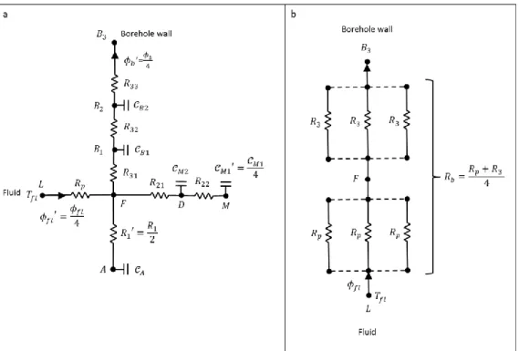
To overcome these obstacles we developed a RC circuit where the concrete is divided in as many zones as pipe in the pile. For the sake of clarity, we limit the paper to the case where the pile is equipped with four pipes (cf. Figure 5). The model can be easily extended to the case there are more pipes.
Figure 5: (a) cross-sectional view of the PHE geometry. (b) The developed RC model.
The RC circuit that we developed has 11 parameters: (i) Six resistances: , , , , , . (ii) Five capacities: , , , , .
Every outer face of a pipe, denoted (i=1,2,3,4) is connected to the opposite portion of the borehole wall by a branch made of three resistances , , . Two capacities and are inserted at the subsequent nodes. This portion of the circuit aims at describing the temperature evolution in the outer part of the pile, i.e. between the pipe and the borehole wall. The choice of the number of resistances and capacities results from a trade-off between an accurate description and a high complexity of the model. Every pipe is connected to the central part of the pile by a branch with two resistances and in the middle of which lies a capacity . Finally, the central part of the pile is represented by a capacity while interactions between two close pipes (such as and ) are accounted for by a capacity lying between two resistances .
To compute the eleven parameters of the RC model we followed a procedure where the underlying idea is to solve the equation in a discretized model and to “tune” the parameters of the RC model to fit the evolution in energy computed by the fully-discretized model. First, the heat equation inside the pile is normalized, so that to decrease the number of relevant parameters, in a similar way to what we did in section 2.2. Second, a set of dynamic simulations characterized by specific boundary conditions are determined. These simulations are run for a FE model developed in COMSOL-Multiphysics; evolution of energy and fluxes are computed for each simulation. In parallel, a RC circuit computing the temperature evolution at the nodes has been developed in the MATLAB software. Finally, parameters of the RC model are determined by fitting the energy computed by the RC model to the energy computed by the FE model.
The Table 2 gives an example of computed values of the RC parameters for a PHE characterized by a radius of 0.3 m. Thermal properties of the pile concrete are similar to the data used by Suryatriyastuti (Suryatriyastuti et al., 2012) and Gashti (Gashti et al., 2014).
Physical parameters of the pile (input data)
Thermal conductivity of the concrete λc
Volume-specific heat capacity of the concrete ( )
Borehole pile radius
rb
Outer radius of the pipe
rp
Distance between two opposite pipes s
1.8 W.K-1.m-1 2.11 MJ.K-1.m-3 0.3 m 0.01 m 0.3 m
Computed RC parameters (output data)
Resistances (K.m.W-1) Capacities (kJ.K-1.m-1)
R1 R2,1 R2,2 R3,1 R3,2 R3,3
2.158 0.135 1.343 0.220 0.119 0.021 6.9 82.0 47.6 32.6 3.9
Table 2: Computed parameters of the RC circuit
2.4 Development of a semi-analytical model to compute the evolution of fluid temperature (SA model)
A numerical semi-analytical model (SA model) has been developed to compute the evolution of temperatures in the fluid, pile and surrounding ground. “Semi-analytical” refers to the fact that the temperature at the pile wall is computed based on a step response G. Therefore, no numerical resolution of the heat equation in the surrounding ground is carried out.
The RC circuit is coupled to a heat balance over the fluid (cf. Figure 6-a). The power exchanged by meter of pile (W.m-1) between the fluid and the surrounding ground at each time step is an input data of the model. A heat balance over the heat carrier fluid gives:
̇
(16)
denotes the depth of the PHE, ̇ the flow rate in the pipe (kg.s-1
), the specific heat capacity of the heat carrier fluid (J.K-1.kg), and the PHE inlet and outlet temperatures respectively. We introduce , a mean temperature of the fluid inside the pipes:
(17)
In the paper we limit to the assumption that the fluid temperature is the same in every pipe. In other words, no thermal “short-circuit” between cold and hot heat-carrier fluid is taken into account. Due to symmetry only one quarter of the RC circuit is modeled. Therefore, at the node L (i.e. at the heat-carrier fluid) the applied power is defined by:
(18) Where Rp denotes the thermal resistance of the pipe.
Figure 6: (a) New semi-analytical model, referred to as “SA” model. (b) One-resistance model, referred to as “1-R” model.
The temperature evolution can be expressed by a heat balance as:
[ ] { } [ ]{ } { } (19)
Where { } is a vector containing the temperature at the eight nodes:
{ } { } (20)
[ ] is the capacity matrix (J.K-1
.m-1), [ ] the conductance matrix (W.K-1.m-1), { } has the dimension of a power vector (W.m-1). [ ], [ ], { } are filled by the heat balance at every node. The temperatures are computed at discretized times tn = n Δt, where Δt is
the time step of the modification. The node B3 deserves a particular attention as it is connected to the ground. To compute its
temperature, we used the superposition principle (Ingersoll and Plass, 1948): ( ∑ ( )
) (21)
Where denotes the step response G evaluated at tk = k Δt. In what follows we used the MICS model, i.e. . The Peclet
number is set to Pe=0. In other words underground water doesn‟t flow ( . is the total heat flux exchanged at the time step k between the pile and the surrounding ground. An algorithm was developed in MATLAB to solve the system of equations (19) with a basic implicit Euler method (Mohammadi and Saïac, 2003).
3. COMPARISON OF THE SEMI-ANALYTICAL MODEL WITH A FINITE-ELEMENT MODEL
A comparison of three models was carried out for parameters given in Table 3:
(i) A numerical model (“FE” model) where the PHE cross-section is fully discretized. The assumption of a homogenous mean fluid temperature remains.
(ii) The semi-analytical model (“SA” model) presented in section 2.4.
(iii) A one-resistance model, where the thermal capacity of the pile is neglected (“1-R” model, cf. Figure 6-b). This model takes into account the cylindrical geometry of the borehole. It lies upon a borehole resistivity Rb given by:
(22) In each model the initial temperature is T0 = 0 K. The power exchanged by meter of pile is set to 50 W.m-1: The fluid cools down while the concrete and ground warm up. 50 W.m-1 is a typical value for thermal response tests (TRT).
PHE characteristics Ground characteristics
Thermal resistance of the pipe Rp
Pile depth H Thermal conductivity of the ground λm Volume-specific heat capacity of the
ground ( )
0.0892 K.m.W-1 10 m 2.3 W.K-1.m-1 2.4 MJ.K-1.m-1
Heat-carrier fluid characteristics PHE solicitation
Specific heat capacity of the fluid Cp,fl Power exchanged by meter of pile
Mass flow rate Temperature difference Duration of the simulation 4180 J.K-1.kg-1 50 W.m-1 0.1 kg.s-1 1.2 K 100 days (2400 h)
Table 3: Parameters of the dynamic simulation. PHE characteristics remain identical to data provided in Table 2.
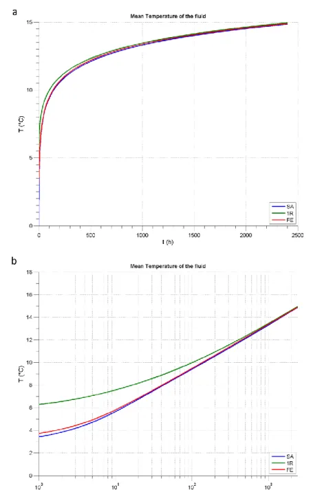
Figure 7 shows the evolutions of the mean temperature fluid Tfl for the three models. It can be emphasized that:
(i) All models converge to the same value at t=100 days. It was expected since once the transient thermal transfer within the pile is over the thermal transfer is driven by conduction in the ground. Each model takes into account the same conductivity λm=2.3 W.K
-1
.m-1 and volume-specific heat capacity of the ground ( ) = 2.4 MJ.K-1.m-3.
(ii) FE and SA models give close results. After one hour, the mean fluid temperature inside the pipes Tfl is respectively
estimated at3.7 K and 3.4 K by the FE and SA models, i.e. a temperature difference of 0.3 K. After 10 hours, the difference reduces to 0.2 K since the models respectively returns 5.6 K and 5.8 K. The good agreement between the two models is an element of validation of the RC circuit, the computation procedure of the RC parameters as well as the development and implementation of the semi-analytical model.
(iii) 1-R model greatly overestimate Tfl compared to FE elements. After one hour, the 1-R model gives 6.3 K against
3.7 K for the FE model, which means an overestimation of almost 2.6 K. After 10 hours, the 1-R model returns 7.6 K against 5.8 K; the overestimation is 1.8 K. It should be kept in mind that these quantitative results are relative to the hypothesis for thermal properties of both concrete and ground (respectively λc=1.8 W.K
-1 .m-1,
( )=2.11 MJ.K-1.m-3 and λm=2.4 W.K
-1
.m-1, ( ) =2.3 MJ.K-1.m-3). However, it seems the 1-R model is not relevant for computation of the temperature evolution over short duration, typically of the order of some hours.
Figure 7: Evolution of mean temperature fluid Tfl computed by the three models in normal scale (a) and in semi-logarithmic
scale (b).
Figure 8 respectively give the evolution of the internal power (W.m-1) of the concrete and of the ground computed by SA and FE models. It can be emphasized that:
(i) For both models, the sum of concrete power and ground power is constant and equal to the applied power (50 W.m-1). This constitutes a verification that both models conserve power.
(ii) Both models give really close evolution of the internal powers. This is an element of validation of the SA model. (iii) At the beginning of the solicitation, is equal to , while is equal to 0, since transient thermal transfer occurs
in the pile concrete and no power is transferred to the surrounding ground. As the time goes, pile concrete warms up and heat starts to be transferred to the surrounding ground through the pile wall; as a consequence increase and
decreases.
(iv) It takes 7.5 hours to reach =25.0 W.m-1, i.e. for the concrete pile to be half loaded. After 20 hours =37 W.m-1, this means that the concrete is loaded at 77 % (=38/50*100). It takes 51 hours for the concrete to be loaded at 95 % (out of the graph). These results suggest that heat transfer in pile heat exchanger is a transient phenomenon that lasts over dozens of hours. It highlights the fact that, depending on the level of precision foreseen, heat transfer in a pile should be treated with relevant models taking into account concrete thermal inertia.
Figure 8: Ground internal power and concrete internal power computed by the SA and FE models for the 40 first hours. 4. CONCLUSION
A new MICS (moving infinite cylindrical source) model has been developed to compute the temperature evolution at the pile wall under steady underground water flow. These step responses GMICS functions are parameterized by the Peclet number Pe, the ratio of
the heat transferred by convection to the heat transferred by conduction. As it accounts for the cylindrical geometry of the pile, the MICS model correctly describes the temperature evolution over the short term. It takes into account the fact the pile is an obstacle to the underground flow and therefore gives higher estimation of the long-term temperature that the MILS (moving infinite line source) model. Our results suggest that the MILS model underestimates the steady-state step responses by 7 % for Pe=0.5 and by 30 % for Pe=1.5 compared to the MICS model.
A resistive-capacitive (RC) circuit has been developed to deal with the thermal inertia of the concrete pile. The parameters of the RC circuit are “tuned” to fit the energy evolution computed by a fully discretized model. The RC circuit has been integrated in a semi-analytical model (SA model) and combined with the GMICS functions to compute the evolution of fluid temperature. The
system of equation is solved with an implicit Euler scheme.
A comparison of the SA model, a fully discretized finite-elements (FE) model and a model that overlooks the thermal capacity of the pile (1-R model) has been carried out. Fluid temperatures computed by the SA and FE models are really close, which is an element of validation of the numerical implementation of the developed SA model. The 1-R model overestimates the fluid temperature compared to the FE and SA models, by 2.6 K after 1 hour, by 1.8 K after 10 hours. Besides, it takes 7.5 hours to half load the pile concrete and it takes 51 hours for the concrete to be loaded at 95 %.
The semi-analytical model seems to be an interesting tool for dynamic simulations of heat pumps connected to pile heat exchangers. In-situ tests achieved in the GECKO project will deliver experimental data to validate this model. Further developments include the computation of RC parameters for a representative number of pipe geometry and equipment, and the integration of the semi-analytical model into an environment of thermal dynamic simulation such as TRNSYS.
5. ACKNOWLEDGEMENT
The work described in this paper is a part of a research project „„GECKO‟‟ (geo-structures and hybrid solar panel coupling for
optimized energy storage) which is supported by a grant from the French National Research Agency (ANR). It is an industrial
project, involving an engineering office, three public companies and two research laboratories in civil and energy engineering sector: ECOME, BRGM, IFSTTAR, CETE Nord Picardie, LGCgE–Polytech‟Lille and LEMTA–INPL. The authors would like to express their gratitude to their partners for their support in this ongoing project.
6. NOMENCLATURE
T temperature (°C) Subscripts
power per meter of pile (W.m-1) b borehole wall
c concrete
thermal conductivity (W.K-1.m-1) ground
Darcy velocity (m.s-1) w underground water
density (kg.m-3) fl heat-carrier fluid
specific heat capacity (J.K-1.kg-1) in inlet volume-specific heat capacity (J.K-1.m-3) out outlet
thermal diffusivity (m².s-1) 0 undisturbed conditions
Fourier number at/rb²
Peclet number
thermal resistance (K.m.W-1) Superscripts
capacity (J.K-1.m-1) * normalized value
̇ flow rate (kg.s-1) n time step n
Acronym
GHE Ground Heat Exchanger PHE Pile Heat Exchanger FE Finite Elements RC Resistive-Capacitive ICS Infinite Cylindrical Source ILS Infinite Line Source
MICS Moving Infinite Cylindrical Source SA Semi-Analytical
REFERENCES
Bauer, D., Heidemann, W., Müller-Steinhagen, H., Diersch: Thermal resistance and capacity models for borehole heat exchangers,
Int. J. Energy Res. 35, (2011), 312–320.
Bourne-Webb P.: Observed Responses of Energy Geostructures, in “Energy Geostructures - Innovation in Underground Engineering”, Wiley (2013), 45-67
Carslaw, H.S., Jaeger, J.C.: Conduction of Heat in Solids, Oxford University Press, Oxford (1947).
Di Donna, A.: Thermo-mechanical aspects of energy piles, PhD thesis of the École polytechnique fédérale de Lausanne EPFL, n° 6145 (2014)
Gashti, E. H., N., Uotinen, V.-M., & Kujala, K: Numerical modelling of thermal regimes in steel energy pile foundations: A case study, Energy and Buildings, 69, (2014), 165–174.
Ingersoll, L.R., Plass, H.J.: Theory of the ground pipe heat source for the heat pump, Heating, Pip. Air Cond., (1948). Laloui, L., Di Donna, A.: Energy Geostructures - Innovation in Underground Engineering, Wiley (2013).
Mohammadi, B., Saïac, J.-H.: Pratique de la simulation numérique, Dunod, Paris (2003).
Observ‟ER: The state of Renewable Energies in Europe - 13th EurObserv‟ER report, Paris (2013).
Shirazi, A.S., Bernier, M.: Thermal capacity effects in borehole ground heat exchangers, Energy Build. 67, (2013), 352–364. SIA: Norme Suisse: Sondes géothermiques SIA 384/6. Société suisse des ingénieurs et des architectes, Zurich (2010)
Suryatriyastuti, M.E., Mroueh, H., Burlon, S.: Understanding the temperature-induced mechanical behaviour of energy pile foundations, Renew. Sustain. Energy Rev, 16, (2012), 3344–3354
Wagner, V., Blum, P., Kübert, M., & Bayer, P.: Analytical approach to groundwater-influenced thermal response tests of grouted borehole heat exchangers. Geothermics, 46, (2013), 22–31.