HAL Id: hal-02403667
https://hal.archives-ouvertes.fr/hal-02403667
Submitted on 2 Dec 2020
HAL is a multi-disciplinary open access
archive for the deposit and dissemination of
sci-entific research documents, whether they are
pub-lished or not. The documents may come from
teaching and research institutions in France or
abroad, or from public or private research centers.
L’archive ouverte pluridisciplinaire HAL, est
destinée au dépôt et à la diffusion de documents
scientifiques de niveau recherche, publiés ou non,
émanant des établissements d’enseignement et de
recherche français ou étrangers, des laboratoires
publics ou privés.
Generation and Derivation of Practical
Optimization-Oriented Models of Inductors
Andrija Stupar, Didier Flumian, Basile Gouedard, Thierry Meynard
To cite this version:
Andrija Stupar, Didier Flumian, Basile Gouedard, Thierry Meynard. Generation and Derivation
of Practical Optimization-Oriented Models of Inductors.
2019 20th Workshop on Control and
Modeling for Power Electronics (COMPEL), Jun 2019, Toronto, Canada. pp.1-8,
�10.1109/COM-PEL.2019.8769669�. �hal-02403667�
Generation and Derivation of Practical
Optimization-Oriented Models of Inductors
Andrija Stupar
Eneropta Corporation Toronto, Canada [email protected]
Didier Flumian, Basile Gouedard, Thierry Meynard´
Laboratoire LAPLACE, ENSEEIHT INPT, University of Toulouse Toulouse,
France
Abstract—Magnetic components contribute significantly to the volume and losses of power electronic systems. Their optimal design is therefore crucial for the overall optimization of power density and efficiency of power converters. Recently it has been shown that converters can accurately be modeled using posynomial functions, thus allowing for the use of Geometric Programming, a type of convex optimization problem, to be used to quickly produce globally optimum designs of entire converter families. Existing studies have however treated magnetic components in a case-specific way, deriving posynomial models suited for the given converter or range of operating points. This paper demonstrates and validates methods for the derivation and generation of posynomial models of inductors for an entire catalogue of standard components, allowing a set of models to be generated once and then re-used subsequently, or “plugged into” an overall converter optimization, repeatedly, without the need for re-derivation.
I. INTRODUCTION
Recently it has been shown [1], [2], [3], [4], [5], that geometric programming [6], a class of convex optimization problems, can be used to accurately and quickly optimize power converters for multiple objectives. There are two main advantages of using this approach. First, in a feasible convex optimization problem, a local minimum is guaranteed to be a global minimum. Second, many efficient solvers for convex optimization problems exist: in [2], [5] it was shown that complex converter topologies can be optimized for efficiency and volume in under one minute. A Geometric Program (GP) has the following form
minimize (1)
subject to
where x = (x1,x2,...,xn) is the vector of design (input) variables, fo(x) is the objective function to be minimized, and fi(x) and hj(x)
are the inequality and equality constraints, respectively, that must be satisfied by the solution. In order for fo(x), fi(x) and hj(x) to
be convex functions, x must be a vector of positive non-zero real numbers, as must be the coefficients (ao,ai,aj), while the
exponents (ko,ki,kj) can be any real number. Such functions are called posynomials (“positive polynomials”) [6].
Therefore, in order to model a power converter as a GP, each component in the system must be modeled using posynomial functions. As shown in [2], [4], [5], semiconductor models are often already in posynomial form or can be manipulated to be in posynomial form in a relatively straightforward manner. Accurate models of magnetic models, such as those in [7], [8], are more difficult to put into posynomial form. In [1], [4], comprehensive posynomial models of inductors were not considered. In [2], [5], low-power SMD inductors were considered and modeled in an application-specific way, with a posynomial model that is appropriate to the converters considered for optimization within the operating range envisioned for the studied application. Therefore, these models cannot be easily transferred to a different converter optimization problem, and in most cases, the models would need to be re-derived. In [3], it was demonstrated that deriving posynomial models of nonSMD custom-built inductors (constructed from standard cores and wires), such as those shown in Fig. 1 was feasible, and a model derivation procedure, based on [9], was presented. However, as [3] was more general in nature and considered other approaches to model derivation as well, the presented example was only a limited proof of concept that also is not easily transferrable to other applications.
This goal of this paper therefore is to present a method for the derivation of re-usable, “generate-once use-multiple-times” posynomial models for higher-power, custom-built inductors made from standard cores, wires, and bobbins. Such a method allows, for a given catalogue of standard parts (cores of a single type of geometry and from the same magnetic material, and
wires of standard gauge from the same conductor material), a set of posynomial functions modeling inductance, peak flux density, total losses, boxed volume, and core and winding temperature to be generated over the entire set of feasible inductors that can be constructed with the considered standard parts. These models can then be reused repeatedly within different converter optimization problems.
In Section II it is shown how such a goal may be attempted to be achieved using analytical equations of inductor geometry based on [10]. While useful results may be obtained with this approach, it is difficult to accurately model winding losses in
(a) Inductor 1 (b) Inductor 2
Fig. 1. Photographs of the built Inductor 1 (EPCOS E55 core, N27 ferrite, 18 turns) and Inductor 2 (EPCOS E32 core, N87 ferrite, 18 turns) used for loss measurements. TABLE I
QUANTITIES OF THE ANALYTICAL POSYNOMIAL INDUCTOR MODEL
fs frequency of the applied square voltage
IDC DC component of the inductor current
ΔI
ΔTmax maximum allowed temperature rise
Kw winding factor (inverse of fill factor)
Kc1,Kc2,α1,α2,β Core loss model parameters
ρ winding resistivity
S thermal exchange area proportion factor
Z,Y winding and core volume proportion factors
JRMS current density, including harmonics of current ripple
gapped cores over a wide range of core geometries and winding arrangements in this manner. Therefore, in Section III, an approach which is a significant extension of the method from [3], using simulation data from a dedicated power electronics inductor simulation tool, is derived and demonstrated. The accuracy of the simulation tool, and therefore its suitability for use as a source of data for the derivation of posynomial models, is confirmed using experimental measurements. The accuracy of the derived models is evaluated using a set of sample optimization problems. The paper is concluded with Section IV.
II. MODEL DERIVATION BASED ON ANALYTICAL
EQUATIONS
Starting from the well-known concept of area product (AeWa – where Ae is the core cross-sectional area and Wa the core winding
window area), in [10], [11], functions describing several different core shapes are derived, with derived geometry-specific correction factors. The resulting models are used in [10] in an iterative transformer design procedure, and in [11] in an iterative inductor design procedure. Most models presented in [10], [11] are in fact in, or close to, posynomial form. Key quantities of these models are summarized in Table I. Each considered core shape is characterized such that the core lengths are proportional to
, the core areas to
, and the core volumes and weights to . Additionaly, a thermal exchange coefficient Htherm is specified as a constant
value to be typical either of natural convection, forced convection, or liquid cooling. For details on the expressions for and values of the quantities in Table I, the reader is directed to [10], [11].
Therefore, a GP can be formulated where the main free variable is the size of the core, i.e. AeWa, along with the induction at
Fig. 2. A Pareto front of optimum inductor designs for a given L, fs, core material and shape for different values of Htherm. nominal current JDC:
minimize AeWa (2)
subject to where L is the desired inductance. The first constraint in (2) is the
inductance requirement, the second constraint is the saturation limit, and the third the thermal limit, i.e. the total amount of allowed losses. Therefore, (2) minimizes the area product of an inductor built from a specified core material and core shape, for
a given upper loss limit and desired inductance. The objective function in (2) could be changed from AeWa to the AeWa-dependent
function for losses, weight or volume given in [10], [11], or to a weighted sum of two or more of these functions, giving a multi-objective problem.
A loss-volume Pareto front can be constructed by repeatedly solving (2) for different values of Htherm, as shown in Fig. 2. This
immediately shows the feasible (theoretically realizable) and non-feasible regions of the inductor design space, showing the minimum volume achievable for different types of cooling. The same can be repeated with different core materials and at different frequencies (as in Fig. 3) or with different core shapes, etc. Since (2) can be solved in a few seconds, it is a powerful tool for the exploration of large design spaces, and can be used to quickly identify which cooling methods, core shapes, core materials, and so on, are appropriate to a particular application or design task.
Unfortunately, this approach is limited when applied to gapped cores. As shown in [7], a general closed-form analytical solution does not exist for proximity losses due to an air gap’s fringing flux, and at least a 2-D summative calculation method must be used instead. The reluctance of an air gap is
s Δ ˚
Fig. 3. Pareto fronts for a given L for different core material and fs pairs.
Fig. 4. The general, structured, successive fitting procedure for deriving posynomial models from data characterizing a family of inductors [9], [3].
also difficult to encapsulate in a simple analytical equation. Therefore an extension of the approach in [10], [11] was developed in [12], using finite element method (FEM) simulations to derive correction factors for ρ that include the effects the air gap on the winding losses. Such correction factors are, however, extremely geometry-dependent and require a large number of FEM simulations to refine. Considering the complexity of the problem, it is simpler to then characterize the entire inductor using a proven, comprehensive power electronics-oriented simulation tool. This different approach is described in detail in the following Section.
III. SIMULATION DATA-BASED MODEL GENERATION
Following [9], [3] presents a procedure, shown in Fig. 4, to fit posynomial functions to data that has been generated by simulations, measurement, or from the evaluation of nonposynomial analytical models. First, the data is partitioned. The number of partitions determines the number of terms in the fitted posynomial functions. Then, to each partition, a monomial function, shown in (3), is fitted separately. The results of the fits for each partition are used as an initial guess for fitting a max-monomial function, shown in (4), to the entire data set. The results of the max-monomial fit are then used as an initial guess for fitting the final posynomial function, shown in (5), to the data.
h(x) = ealx1kl1...xnkln (3)
(4)
m n
f(x) = eal xikli (5)
l=1 i=1
It should be noted that monomial and posynomial functions must be converted to their logarithmic form in order to become convex. Taking the logarithm of both sides in (3) transforms the monomial into a linear (affine) function, the max-monomial in (4) into a max-affine function, and the posynomial in (5) into a softmax-affine function. In the procedure of Fig. 4, the logarithm of the data to be fitted is also taken and fitting is performed to the logarithmic forms of the functions. For more details, the reader is directed to [3] and [9].
In this section, the method presented in [3] is extended to generate posynomial models covering an entire family of potential inductor components, that can be built from cores of the same shape and material but different dimensions, and a standard range of copper wires.
A. Experimental Verification
To generate data for fitting, the magnetic simulation software tool GeckoMAGNETICS [13], version 1.5.0, was selected. It is based on advanced, published models that have been experimentally verified [7], [8], [14], [15]. It contains measurements of core losses with rectangular voltage excitations and DC bias current, allowing for accurate core loss and temperature calculations, and a detailed air gap reluctance model allowing for accurate inductance, winding loss and temperature calculations. To confirm the accuracy of the version of the software used, a measurement setup, shown in Fig. 5, was constructed. The inductor being measured is the device under test (DUT) in Fig. 5 and it is placed between two switching cells.
Cell 2 operates in open loop and generates a quasi-constant voltage Vf across the LC filter. Cell 1, switching at switching period
Ts, generates a square wave voltage vout ranging from 0 to Vin. It operates in closed loop in order to ensure a given current IDC
through the DUT. Therefore by adjusting the operation of the two cells, a current waveform with a peak to peak ripple ΔiL, as
shown in Fig. 6 can be imposed on the DUT. In this way the measurement setup can mimic, from the point of view of the DUT, the behaviour of several different buck- and boost-type converter topologies.
The loss measurement was performed in a manner similar
Fig. 5. Schematic of the measurement setup used to measure inductor losses to verify the accuracy of the GeckoMAGNETICS software.
Fig. 6. The waveform imposed on the DUT by the measurement setup of Fig. 5, with a duty ratio of D and a switching frequency fs =1/Ts.
to that presented in [7], [8]. Total DUT losses were measured using a Yokogawa WT3000 Precision Power Analyzer. The total power
Ptotal is given as
(6)
and was measured across the main inductor winding N1. Additionaly, a second sense winding N2 was added in order to measure
core losses PCore only, given as
(7)
where v2 is the voltage across N2. Winding losses were determined by subtracting PCore from PTotal, and additionally by measuring
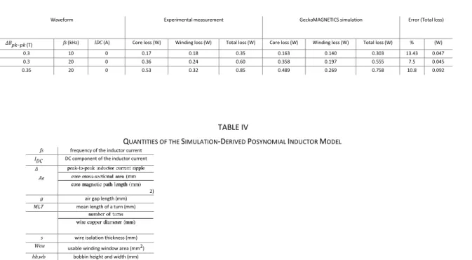
the DC and AC resistance of the winding using a Hioki IM3533 LCR meter. Measurements were performed on Inductor 1, the characteristics of which are shown in Fig. 7 and the built prototype in Fig. 1(a), and Inductor 2, the characteristics of which are shown in Fig. 8 and the built prototype in Fig. 1(b). A selection of the performed measurements and their comparison to GeckoMAGNETICS simulations for the two inductors is shown in Table II and Table III, respectively. It can be seen that the agreement between measurements and simulations is very good. Therefore, GeckoMAGNETICS is an appropriate tool to use to generate data for the derivation of posynomial inductor models.
L s s Δ
B. Data Generation
In order to generate posynomial models that can be used over a wide variety of applications, the entire catalogue of TDK EPCOS EE cores (ranging from E13 to E55) made from
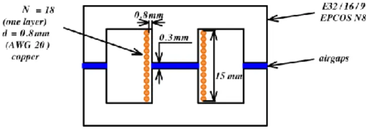
Fig. 7. Specifications of the Inductor 1 DUT, built from an EPCOS E55 core and N27 ferrite material.
Fig. 8. Specifications of the Inductor 2 DUT, built from an EPCOS E32 core and N87 ferrite material.
the N87 ferrite was selected for simulation. The cores were not stacked, and only cores with a built-in centre air gap, ranging from 0.04 mm to 2 mm, were selected. To construct the windings, standard American wire gauge (AWG) solid copper wires were used, ranging from AWG10 to AWG44. The dimensions shown in Fig. 9 and Table IV were used to characterize an inductor. An algorithm was designed to generate a set of feasible inductors over the entire range of the parts catalogue. A maximum
allowable current density of Jmax = 4 A/mm2 was assumed. Fill factor was kept between 0.1 and 0.6. For each core (including air
gap), the core reluctance Rtot was calculated using GeckoMAGNETICS. Assuming first N = 1, and using the core material’s
saturation flux density Bsat, the peak allowable current for the inductor was calculated using
. (8)
From this, the smallest wire diameter dmin that can accommodate Ipk,max while respecting the limit on Jmax was calculated as
. (9)
To construct the inductor, the next largest AWG wire was
Fig. 9. The physical dimensions used to characterize an inductor.
TABLE II MEASUREMENT RESULTS FOR INDUCTOR 1
Waveform Experimental measurement GeckoMAGNETICS simulation Error (Total loss)
ΔBpk−pk (T) fs (kHz) IDC (A) Core loss (W) Winding loss (W) Total loss (W) Core loss (W) Winding loss (W) Total loss (W) % (W) 0.2 10 0 0.45 0.28 0.73 0.483 0.336 0.818 12.05 0.088 0.3 10 0 1.14 0.65 1.79 1.071 0.751 1.822 1.79 0.032 0.5 5 0 1.56 1.11 2.67 1.271 0.961 2.232 16.4 0.438
TABLE III MEASUREMENT RESULTS FOR INDUCTOR 2
TABLE IV
QUANTITIES OF THE SIMULATION-DERIVED POSYNOMIAL INDUCTOR MODEL
fs frequency of the inductor current
IDC DC component of the inductor current
Δ Ae
2)
g air gap length (mm)
MLT mean length of a turn (mm)
s wire isolation thickness (mm)
Wau usable winding window area (mm2) hb,wb bobbin height and width (mm)
selected. A series of inductors was then constructed with the same number of turns but using every AWG wire size that respected the limits on the fill factor. When the number of possible designs was exhausted, N was incremented to 2 and then the entire procedure was repeated, and so on, until N = 50. For each core in the catalogue, this then created the entire set of feasible designs that could be constructed with AWG solid copper wires with up to 50 turns.
At the first attempt this generated a very large number of very similar inductor designs. In order to reduce the amount of designs to simulate, designs using adjacent AWG wire sizes were discarded (for example, designs using AWG10, AWG12, and AWG14 were selected for simulation, but not those with AWG11 and AWG13). This was acceptable since the difference between adjacent AWG wire dimeters is only about 11%. Similarly, an additional turn produces a much larger change inductance when added to a low number of turns than when added to a large number of turns. For this reason, the number of turns was incremented by 1 until N = 10, then by 2 until N = 20, and by 5 thereafter. This finally produced a total of 880 inductor designs, with inductance L ranging from 1 µH to 4 mH. The generated designs therefore spanned the entire set of applications appropriate to this catalogue of cores. For all simulations, an ambient temperature of 25°C was assumed. Each inductor was simulated using triangular current
waveforms, such as those shown in Fig. 6, with 50% duty ratio and different average current IDC and peak-to-peak current ripple
ΔiL. For each inductor, IDC was selected to be 0.1, 0.3, 0.6, and 0.8 of the Ipk,max for that inductor. ΔiL was then selected to be 0.1,
0.2, 0.4, 0.6, and 0.9 of the selected values of IDC. Waveform frequencies fs were selected to be 20, 50, 100, and 200 kHz, as that
was the range within which the GeckoMAGNETICS tool contained accurate core loss data. Taking together all of the generated inductors, this produced 63360 valid simulations. For each simulated inductor, besides the geometry characteristics shown in Fig.
9 and the previously detailed waveform characteristics, the peak flux density Bpk, total losses PTotal, core temperature Tcore, winding
temperature Twind, and boxed volume V olbox were recorded. The simulations took about 15 hours to complete on a low to
mid-range laptop computer using a single thread of execution.
C. Posynomial Fitting
Following the approach of [3], data was divided into four partitions based on waveform frequency fs. Each partition had the
same frequency value. The successive fitting method was used to produce a four-term posynomial for the total losses Ptotal (in
mW) and the core and winding temperature Tcore and Twind, respectively (in °C):
4
PTotal =(ealpAeklp1leklp2Wauklp3dklp4sklp5MLTklp6Nklp7 lp=1
· gklp8fsklp9ΔiLklp10IDCklp11) (10)
Waveform Experimental measurement GeckoMAGNETICS simulation Error (Total loss)
ΔBpk−pk (T) fs (kHz) IDC (A) Core loss (W) Winding loss (W) Total loss (W) Core loss (W) Winding loss (W) Total loss (W) % (W) 0.3 10 0 0.17 0.18 0.35 0.163 0.140 0.303 13.43 0.047 0.3 20 0 0.36 0.24 0.60 0.358 0.197 0.555 7.5 0.045 0.35 20 0 0.53 0.32 0.85 0.489 0.269 0.758 10.8 0.092
4
Tcore =(ealcAeklc1leklc2Wauklc3dklc4sklc5MLTklc6Nklc7 lc=1
· gklc8fsklc9ΔiLklc10IDCklc11) (11)
4
Twind =(ealw Aeklw1leklw2Wauklw3dklw4sklw5MLTklw6 lw=1
· Nklw7gklw8fsklw9ΔiLklw10IDCklw11) (12) The exponent values for (10) - (12) are shown in Table V.
However, for the inductance L (µH), peak flux density Bpk (mT), and boxed volume V olbox (cm3) it was sufficient to fit just a
monomial function to the entire data set:
L = e−5.82Ae0.839le0.062N2g−0.722 (13)
Bpk = e1.083le−0.269N0.997g−0.785ΔiL1.0026IDC−0.00486
(14)
V olbox =e−22.42Ae−3.08le2.14Wau−1.28d0.528s−0.0156
· MLT8.97N0.243g−0.00294. (15)
L must be a monomial in order to be included into a GP as an equality constraint. Since inductance is physically a function of the
number of turns and the core geometry, a
monomial function of Ae, le, g, and N can be fitted with high accuracy. Similarly, V olbox is also a function only of the inductor’s
dimensions, so the variables related to the applied waveform can be ommitted. The form of the function for Bpk was determined
by trial and error based on the intuition that it should depend only on the inductor geometry and the peak current.
The fitting was performed using least-squares functions in MATLAB and took about 30 minutes to execute on the same computer which was used to produce the simulation data. As can be seen in Table VI, the produced posynomial functions fit quite well to
the simulation data. The highest error, but still less than 10%, is present when fitting Ptot, which is understandable taking into
consideration the complexity of accurate inductor loss modeling.
D. Alternative Partitioning Approaches
In addition to the approach of the previous subsection, different partitioning schemes were considered. First, the frequency-sorted data was divided into two partitions, with each partition containing two adjacent values of frequency. Then the data was
sorted according to Bpk ascending, and divided into four partitions. The data contained nine different values of Ae, so three core
geometry-based partitions were created, each containing three adjacent values of Ae. Finally, the successive fitting approach of
Fig. 4 was discarded and a posynomial with 2, 3, and 4 terms was fitted directly to the simulation data without any partitioning
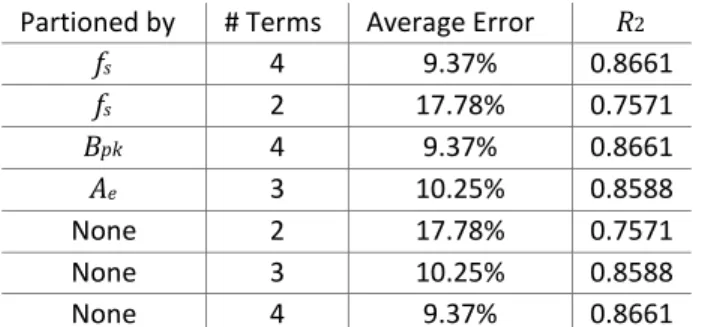
(the data was sorted by fs ascending). The results of the different approaches are compared in Table VII using the fitting error for
the total losses. The fitting errors for Tcore and Twind follow broadly the same trend. The sorting of the data did not have any effect
on the fitting results of the monomial functions, as identical outcomes were achieved for them in each case.
Interestingly, the 4-term Bpk partition produces an identical error as the 4-term fs partition and the 4-term non-partitioned data,
although with different exponent values. The same relationship holds between the 2-term fs partition and 2-term nonpartitioned
results, as well as between the 3-term Ae partition and the 3-term non-partitioned results. This suggests that the number of terms,
and not the sorting and the partioning of the data, is most important, with a higher number of terms producing a better fit.
E. Optimization Example
To demonstrate the use of the derived posynomial models, an inductor with L = 100 µH, operating at fs = 36 kHz, ΔiL =
TABLE V
EXPONENT VALUES FOR PTotal, Tcore, AND Twind FITS
PTotal Tcore Twind a1 -25.9732 248.0399 27.0296
k11 -2.9014 66.7886 7.7489 k12 2.1662 -12.7809 -1.9070 k13 -1.7791 26.8207 3.3015 k14 0.5600 -0.3203 -0.7791 k15 0.3944 0.6059 1.3365 k16 7.2951 -174.6128 -19.3796 k17 2.5932 11.7956 1.2532 k18 0.2473 -9.0848 -0.9883 k19 0.6617 0.9039 0.6758 k110 2.0082 3.4054 1.1878 k111 -0.0435 8.3293 0.1596 a2 171.9199 12.1514 -6.3509 k21 52.8727 5.5936 2.5028 k22 -6.8350 -1.3211 2.1783 k23 20.8084 2.2491 -0.0768 k24 -0.0674 -0.1623 1.3027 k25 -0.0355 0.1870 -2.0040 k26 -138.7475 -13.4502 -8.0003 k27 11.9716 1.3202 2.0799 k28 -9.1608 -1.1549 0.2497 k29 1.0854 0.7037 0.4624 k210 3.5435 1.3332 1.4654 k211 8.3084 0.0262 0.0447 a3 -10.3364 19.6335 2.4875 k31 3.4004 8.6238 -0.1779 k32 -0.0813 1.0635 0.0316 k33 0.8497 1.8095 -0.0751 k34 -0.0999 2.3180 0.0072 k35 0.2385 -2.9849 -0.0039 k36 -6.0294 -23.6927 0.4638 k37 2.2013 2.0271 -0.0164 k38 -1.7766 0.4142 0.0083 k39 1.0828 0.3862 -0.0063 k310 2.2052 1.0735 -0.0121 k311 0.0031 0.2321 -0.0049 a4 -6.5900 2.7913 16.1347 k41 -0.8898 -0.1711 3.7509 k42 -0.6872 0.0319 -0.6237 k43 -0.3636 -0.0751 1.4514 k44 -1.4864 -0.0105 -1.6475 k45 -0.2330 0.0072 -0.7248 k46 3.6423 0.4345 -10.2363 k47 1.1712 -0.0359 0.5925 k48 0.0047 0.0283 0.0505 k49 0.0125 -0.0186 -0.1289 k410 0.0615 -0.0325 -0.1782 k4 1.9857 0.0020 1.8727 11 TABLE VI
ERROR OF FITTED POSYNOMIAL FUNCTIONS WITH RESPECT TO THE SIMULATION DATA
Function Average
Error
R2
Total losses PTotal 9.37% 0.8661
Core temperature Tcore 2.34% 0.9507
Twind 1.66% 0.978
L
0.62% 0.9998
Bpk 3.5% 0.9965
1.67 A, and IDC = 3 A was optimized for losses and volume. Core and winding temperature were limited to be at most 100°C. As
in [5], the two conflicting objectives were weighted by a factor γ and added into a single objective function. Since loss and volume are calculated in different units, they were normalized to a range between 0 and 1. To achieve this,
TABLE VII
ERRORS OF DIFFERENT PARTITIONING APPROACHES (PTotal)
Partioned by # Terms Average Error R2
fs 4 9.37% 0.8661 fs 2 17.78% 0.7571 Bpk 4 9.37% 0.8661 Ae 3 10.25% 0.8588 None 2 17.78% 0.7571 None 3 10.25% 0.8588 None 4 9.37% 0.8661
first the volume was minimized in a single-objective problem, and due to the inverse relationship of the volume and losses of
Pareto-optimal solutions [16], the losses of the minimum volume design, Ptot,max, were used to normalize the losses in the
multi-objective problem. Similarly, loss was minimized in a single-multi-objective problem as well, and the volume of the minimum-loss solution, V olbox,max, was used to normalize the volume in the multi-objective problem. This gave the final multi-objective GP formulation:
minimize (16)
subject to L = e−5.82Ae0.839le0.062N2g−0.722
Tcore ≤ 100◦C
Twind ≤ 100◦C
Bpk ≤ Bsat Ae,min ≤ Ae ≤ Ae,max le,min ≤ le ≤ le,max
Wau,min ≤ Wau ≤ Wau,max dmin ≤ d ≤ dmax smin ≤ s ≤ smax MLTmin ≤ MLT ≤ MLTmax Nmin ≤ N ≤ Nmax gmin ≤
g ≤ gmax
d ≥ 2(((IDC + 0.5ΔiL)/Jmax)/π)0.5
0.1 ≤ Nπ((0.5d)2)/Wau ≤ 0.6 MLT = 5.793Ae0.4723 le = 7.196(Wau0.5184)
Ae = 0.0006963(le2.683), where the design variables – the geometric parameters – were constrained to be within
the minimum and maximum bounds found in the generated simulation data. Additional constraints were added to keep the current density and fill factor of the optimized designs within the limits of the simulated data as well. This however was not sufficient to force the GP to produce inductor designs using the desired core catalogue, as in the absence of further constraints,
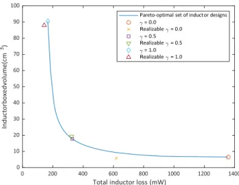
Fig. 10. The resulting Pareto-optimal set of inductors for the example optimization problem. TABLE VIII REALIZABLE OPTIMUM INDUCTORS
γ 0.0 0.5 1.0
Core E20 E32 E55
Air gap (mm) 0.5 0.5 0.5
Wire AWG18 AWG14 AWG10
N 28 19 10
Since the winding is wound around the centre core leg in this case, MLT depends on Ae, which is defined by the centre leg.
Similarly, le depends on the size of Wau. Therefore two monomial expressions, giving MLT as a function of Ae, and le as a function
of Wau, were derived by fitting to the simulation data, and added to the GP as equality constraints. A third monomial constraint
relating Ae to le was derived in the same manner in order to force the GP to produce cores with roughly the same proportions as
those available in the actual core catalogue.
The GP (16) was solved in MATLAB using CVX [17] and the SeDuMi solver. 21 GPs total were solved, with each corresponding to a value of γ ranging from 0 to 1, incremented by 0.05. Execution time was under one minute. The resulting loss-volume Pareto front is shown in Fig. 10. Three points are indicated on the Pareto front, γ = 0, corresponding to the most compact (minimum volume) design, γ = 1, corresponding to the most efficient (minimum loss) design, and γ = 0.5, corresponding to the halfway compromise between the two. Based on the characteristics of these designs, realizable inductors, shown in Table VIII, were built using the cores and wires of the initially simulated catalogue, and then re-simulated in GeckoMAGNETICS. The results of those simulations are also shown in Fig. 10. Note that the plotted values for the realizable designs are directly from GeckoMAGNETICS simulations, and not from the posynomial models, therefore the difference between them and the optimized curve includes the model error from Table VI. The total losses and boxed volumes given by the GP results, the realizable inductors evaluated using the fitted posynomial functions, and the GeckoMAGNETICS simulations are compared in Table IX. It can be seen that for γ = 0.5 and γ = 1.0, the realizable designs are extremely close to the theoretical optima resulting from the GP. For γ = 0, the volume of the realizable design is very close to the theoretical one, which is most important in this case, as this is the minimum volume design. However, there is a large discrepancy in the losses, with the losses of the realizable design being significantly lower than that of the theoretical design. As can be seen in Table IX, this large discrepancy shows up between the posynomial loss model’s calculation and the GeckoMAGNETICS simulation. This is due to a larger fitting error in the area of the data around the selected core. The error reported in Table VI is an average value and there are sections of the data where it is both significantly larger and smaller than the average.
TABLE IX
COMPARISON OF OPTIMIZED INDUCTOR DESIGNS: GP SOLUTIONS VS. REALIZABLE INDUCTORS
γ 0.0 0.5 1.0
PTotal (mW) Volbox (cm3) PTotal (mW) Volbox (cm3) PTotal (mW) Volbox (cm3)
GP result (ideal inductor) 1328 6.522 326 17.924 167 89.38 Realizable inductor, posynomial function evaluation 1154 5.508 338 19.943 185 91.48 Realizable inductor, GeckoMAGNETICS simulation 619 5.807 324 19.321 143 87.93
F. Future Improvements
As noted, the error distribution of the fitted functions is not uniform throughout the data set. Therefore, it would be desireable to add a third metric evaluating the goodness of the fit with respect to the error distribution, and to compare the different fits in Table VII accordingly. Also, all of the presented models were derived from simulations using a fixed ambient temperature, and as a next step the ambient temperature should be added to the posynomial functions for
PTotal, Tcore, and Twind.
Finally, as noted, all of the simulations were performed using waveforms with a 50% duty ratio. Preliminary investigations performed on the results of the optimization example show that changing the duty ratio changes the loss simulation results noticeably but not significantly. It would therefore be necessary to rigorously quantify the effect of the duty ratio and determine whether is necessary to include it as a variable in the above-mentioned posynomial functions.
IV. CONCLUSIONS
Geometric programming, which operates on functions in posynomial form, is a powerful framework for the multiobjective optimization of power electronics. Previous studies, while showing that converters can be modeled as GPs, have not produced “portable” models of inductors, meaning that a re-derivation of posynomial inductor models was required for each new optimization problem. In this paper, an approach has been presented to mitigate this shortcoming, allowing comprehensive posynomial models of inductors to be generated once from simulation data and re-used in different applications.
REFERENCES
[1] U. Ribes-Mallada, R. Leyva, and P. Garces. ”Optimization of DC-DC´ Converters via Geometric Programming”. Mathematical Problems in Engineering, 2011(Article ID 458083):1–19, July 2011.
[2] A. Stupar, T. McRae, N. Vukadinovic, A. Prodi´ c, and J. Taylor. ”Multi-´ objective optimization and comparison of multi-level DC-DC converters using convex optimization methods”. In Proc. 2016 18th European Conference on Power Electronics and Applications (EPE’16 ECCE Europe), Karlsruhe, Germany, September 2016.
[3] A. Stupar, J. Taylor, and A. Prodic. ”Posynomial Models of Inductors for´ Optimization of Power Electronic Systems by Geometric Programming”. In Proc.
2016 IEEE Workshop on Control and Modeling for Power Electronics (COMPEL 2016), Trondheim, Norway, June 2016.
[4] A. Stupar, M. Halamicek, T. Moiannou, A. Prodic, and J. Taylor.´ ”Efficiency Optimization of a 7-Switch Flying Capacitor Buck Converter Power Stage IC Using Simulation and Geometric Programming”. In Proc. 2018 IEEE Workshop on Control and Modeling for Power Electronics (COMPEL 2018), Padova, Italy, June 2018.
[5] A. Stupar, T. McRae, N. Vukadinovic, A. Prodi´ c, and J. Taylor. ”Multi-´ Objective Optimization of Multi-Level DC-DC Converters using Geometric Programming”. IEEE Transactions on Power Electronics, April 2019. Early access: DOI 10.1109/TPEL.2019.2908826.
[6] S. Boyd, S.-J. Kim, L. Vandenberghe, and A. Hassibi. “A tutorial on geometric programming”. Optim Eng, 8:67–127, April 2007.
[7] J. Muhlethaler.¨ Modeling and Multi-Objective Optimization of Inductive Power Components. PhD thesis, Swiss Federal Institute of Technology (ETH Zurich), 2012. Diss. Nr. 20217.¨
[8] J. Muhlethaler, J. Biela, J. W. Kolar, and A. Ecklebe. ”Improved Core-¨ Loss Calculation for Magnetic Components Employed in Power Electronic Systems”.
IEEE Transactions on Power Electronics, 27(2):964– 973, February 2012.
[9] W. Hoburg, P. Kirschen, and P. Abbeel. ”Data Fitting with GeometricProgramming-Compatible Softmax Functions”. Optimization and Engineering, 17(4):897 – 918, August 2016.
[10] F. Forest, E. Laboure, T. Meynard, and M. Arab.´ ”Analytic Design Method Based on Homothetic Shape of Magnetic Cores for HighFrequency Transformers”. IEEE Transactions on Power Electronics, 22(5):2070 – 2080, September 2007.
[11] F. Forest, E. Laboure, T. Meynard, and V. Smet. ”Design and Com-´ parison of Inductors and Intercell Transformers for Filtering of PWM Inverter Output”.
IEEE Transactions on Power Electronics, 24(3):812 – 821, March 2009.
[12] A. Furlan, A. Morentin, G. Fontes, G. Delamare, M. L. Heldwein, and T. Meynard. ”Homothetic Method to Compute Winding Losses in the Design of Power Inductors”. In Submitted for publication at IECON 2019, 2019.
[13] GeckoMAGNETICS modeling and design tool for magnetic components for power electronics, http://geckosimulations.com/geckomagnetics.html. [14] J. Muhlethaler.¨ Measurement Results (Losses and Temperature) - GeckoMAGNETICS, http://geckosimulations.com/downloads/GeckoM acc.pdf, March
2015.
[15] J. Muhlethaler¨ and A. Stupar. Inductance Measurement Results - GeckoMAGNETICS,
http://geckosimulations.com/images/InductanceMasurementWhitePaper.pdf, July 2015.
[16] J. Biela, D. Hassler, J. Minibock, and J. W. Kolar. “Optimal Design of a¨ 5kW/dm3 / 98.5% Efficient TCM Resonant Transition Single-Phase PFC Rectifier”. In Proc. of the IEEE/IEEJ International Power Electronics Conference (ECCE Asia 2010), pages 1709 – 1716, Sapporo, Japan, June 2010.