Theoretical Analyses of Cross-Validation Error and Voting in Instance-Based Learning

Publisher’s version / Version de l'éditeur:

Journal of Experimental and Theoretical Artificial Intelligence (JETAI), 6, 1994

READ THESE TERMS AND CONDITIONS CAREFULLY BEFORE USING THIS WEBSITE. https://nrc-publications.canada.ca/eng/copyright

Vous avez des questions? Nous pouvons vous aider. Pour communiquer directement avec un auteur, consultez la

première page de la revue dans laquelle son article a été publié afin de trouver ses coordonnées. Si vous n’arrivez pas à les repérer, communiquez avec nous à PublicationsArchive-ArchivesPublications@nrc-cnrc.gc.ca.

Questions? Contact the NRC Publications Archive team at

PublicationsArchive-ArchivesPublications@nrc-cnrc.gc.ca. If you wish to email the authors directly, please see the first page of the publication for their contact information.

Archives des publications du CNRC

This publication could be one of several versions: author’s original, accepted manuscript or the publisher’s version. / La version de cette publication peut être l’une des suivantes : la version prépublication de l’auteur, la version acceptée du manuscrit ou la version de l’éditeur.

Access and use of this website and the material on it are subject to the Terms and Conditions set forth at

Theoretical Analyses of Cross-Validation Error and Voting in Instance-Based Learning

Turney, Peter

https://publications-cnrc.canada.ca/fra/droits

L’accès à ce site Web et l’utilisation de son contenu sont assujettis aux conditions présentées dans le site LISEZ CES CONDITIONS ATTENTIVEMENT AVANT D’UTILISER CE SITE WEB.

NRC Publications Record / Notice d'Archives des publications de CNRC:

https://nrc-publications.canada.ca/eng/view/object/?id=82cd15e5-9759-403c-b307-f0ea24165970 https://publications-cnrc.canada.ca/fra/voir/objet/?id=82cd15e5-9759-403c-b307-f0ea24165970

Theoretical Analyses of Cross-Validation Error and

Voting in Instance-Based Learning

Peter Turney

Knowledge Systems Laboratory

Institute for Information Technology

National Research Council Canada

Ottawa, Ontario, Canada

K1A 0R6

613-993-8564

peter@ai.iit.nrc.ca

Theoretical Analyses of Cross-Validation Error and

Voting in Instance-Based Learning

Abstract

This paper begins with a general theory of error in cross-validation testing of algorithms for supervised learning from examples. It is assumed that the examples are described by attribute-value pairs, where the values are symbolic. Cross-validation requires a set of training examples and a set of testing examples. The value of the attribute that is to be predicted is known to the learner in the training set, but unknown in the testing set. The theory demonstrates that cross-validation error has two components: error on the training set (inaccuracy) and sensitivity to noise (instability).

This general theory is then applied to voting in instance-based learning. Given an example in the testing set, a typical instance-based learning algorithm predicts the desig-nated attribute by voting among the k nearest neighbors (the k most similar examples) to the testing example in the training set. Voting is intended to increase the stability (resis-tance to noise) of ins(resis-tance-based learning, but a theoretical analysis shows that there are circumstances in which voting can be destabilizing. The theory suggests ways to minimize cross-validation error, by insuring that voting is stable and does not adversely affect accuracy.

1 Introduction

This paper is concerned with cross-validation testing of algorithms for supervised learning from examples. It is assumed that the examples are described by attribute-value pairs, where the attributes can have a finite number of symbolic values. The learning task is to predict the value of one of the attributes, given the value of the remaining attributes. It is assumed that each example is described by the same set of attributes.

Without loss of generality, we may assume that the attributes are restricted to boolean values. Let us suppose that each example has attributes. We may think of an example as a boolean vector in the space . The learning task is to construct a function from to , where is the space of the predictor attributes and is the space of the attribute that is to be predicted.

Cross-validation testing requires a set of training examples and a set of testing

r+1 0 1

{ , }r+1 0 1

examples. The learning algorithm (the student) is scored by a teacher, according to the student’s performance on the testing set. The teacher knows the values of all of the attributes of all of the examples in the training set and the testing set. The student knows all of the values in the training set, but the student does not know the values of the attribute that is to be predicted in the testing set. The student uses the training set to develop a model of the data. The student then uses the model to make predictions for the testing set. The teacher compares the student’s predictions with the actual values in the testing set. A mismatch between the student’s prediction and the actual value is counted as an error. The student’s goal is to minimize the number of errors that it makes on the testing set.

In a recent paper (Turney, 1993), a general theory of error in cross-validation testing of algorithms for predicting real-valued attributes is presented. 1 Section 2 of this paper extends the theory of Turney (1993) to algorithms for predicting boolean-valued attributes. This section shows that cross-validation error has two components: error on the training set and sensitivity to noise. Error on the training set is commonly used as a measure of accuracy (Fraser, 1976). Turney (1990) introduces a formal definition of

stability as a measure of the sensitivity of algorithms to noise. Section 2 proves that

cross-validation error is bounded by the sum of the training set error and the instability. The optimal cross-validation error is established, and it is proven that the strategy of minimiz-ing error on the trainminimiz-ing set (maximizminimiz-ing accuracy) is sub-optimal.

Section 3 examines the cross-validation error of a simple form of instance-based learning (Aha et al., 1991; Kibler et al., 1989). Instance-based learning is not a single learning algorithm; it is a paradigm for a class of learning algorithms. It is related to the nearest neighbor pattern classification paradigm (Dasarathy, 1991). In instance-based learning, the student’s model of the data consists of simply storing the training set. Given an example from the testing set, the student makes a prediction by looking for similar examples in the training set. Section 3 proves that this simple form of instance-based learning produces sub-optimal cross-validation error.

Looking for the single most similar example is sub-optimal because it is overly sensitive to noise in the data. Section 4 deals with instance-based learning algorithms that look for the k most similar examples, where . In general, the k most similar examples will not all agree on the value of the attribute that is to be predicted. This section examines algorithms that resolve this conflict by voting (Dasarathy, 1991). For example, suppose and the value of the attribute that is to be predicted is 1 for two of the three examples and 0 for the remaining example. If the algorithm uses majority voting, then the prediction is that the value is 1.

k≥1

Section 4 presents a detailed theoretical analysis of voting in instance-based learning. One motivation for voting is the desire to make instance-based learning more stable (more resistant to noise in the data). This section examines the stability of voting in the best case, the worst case, and the average case. It is shown that, in the worst case, voting can be

destabilizing. That is, in certain circumstances, voting can actually increase the sensitivity

to noise.

Section 5 discusses the practical application of this theory. It is shown how it is possible to estimate the expected cross-validation error from the training set. This section presents estimators that can indicate whether voting will increase or decrease stability for a particular set of data. This gives a method for choosing the value of k that will minimize the cross-validation error.

Section 6 compares the work presented here with related work. The most closely related work is Turney (1993), which first introduced many of the concepts used here. There are interesting differences, which arise because Turney (1993) involves real-valued attributes and classes, while this paper involves boolean-valued attributes and classes. This theory is closely related to Akaike Information Criterion statistics (Sakamoto et al., 1986), as is discussed elsewhere (Turney, 1993). There is also an interesting connection with some prior work in nearest neighbor pattern classification (Cover & Hart, 1967).

Finally, Section 7 considers future work. One weakness of this general theory of cross-validation error is that it does not model interpolation and extrapolation. Another area for future research is applying the theory to problems other than voting in instance-based learning.

2 Cross-Validation Error

This section presents a general theory of error in cross-validation testing of algorithms for predicting symbolic attributes. In order to make the exposition simpler, the discussion is restricted to boolean-valued attributes. It is not difficult to extend the results presented here to n-valued attributes, where n is any integer larger than one.

2.1 Exclusive-Or

This paper makes extensive use of the boolean exclusive-or operator. Suppose x and y are boolean variables. That is, x and y range over the set . We may write for “x exclusive-or y”. The expression has the value 1 if and only if exactly one of x and y has the value 1. Here are some of the properties of exclusive-or:

0 1

{ , } x⊕y x⊕y

(1) (2) (3) (4) (5) (6)

These properties can easily be verified with a truth-table.

The following results use exclusive-or with boolean vectors. Suppose and are boolean vectors in the space . The expression represents the vector that results from applying exclusive-or to corresponding elements of and :

(7)

(8)

(9)

(10)

2.2 Accuracy and Stability

Suppose we have a black box with r inputs and one output, where the inputs and the output can be represented by boolean values. Let the boolean vector represent the inputs to the black box:

(11)

Let y represent the output of the black box. Suppose that the black box has a deterministic component f and a random component z. The deterministic component f is a function that maps from to . The random component z is a random boolean variable. The probability that z is 1 is p. The probability that z is 0 is . The black box is represented by the equation:

(12)

The variable p is a probability in the range .

x⊕0 = x x⊕1 = ¬x x⊕y = y⊕x x⊕x = 0 x⊕¬x = 1 x⊕ (y⊕z) = (x⊕y) ⊕z x y 0 1 { , }n x⊕y x y z = x⊕y x = x₁ … x_n y = y₁ … y_n z = x₁⊕y₁ … x_n⊕y_n v v = x₁ … x_r 0 1 { , }r { , }0 1 1−p y = f v( )⊕z 0 1 [ , ]

If p is close to 0, then z is usually 0, so the deterministic component dominates and the output y is usually (see equation (1) above). If p is close to 1, then z is usually 1, so the output is usually (see (2)). We may think of p as the probability that will be randomly negated. If p is 0.5, then the random component z completely hides the deter-ministic component f. When p is between 0.5 and 1.0, will be negated more often than not. When we know that p is greater than 0.5, we can negate the output of the black box:

(13)

This counteracts the expected negation of by the random component z. In (12) the output y is with probability . In (13) the output y is with probability p.

Suppose we perform a series of n experiments with the black box. We may represent the inputs in the n experiments with a matrix X:

(14)

Let the i-th row of the matrix X be represented by the vector , where:

(15)

The vector contains the values of the r inputs for the i-th experiment. Let the j-th column of the matrix X be represented by the vector , where:

(16)

The vector contains the values of the j-th input for the n experiments. Let the n outputs be represented by the vector , where:

f v( ) f v( ) ¬ f v( ) f v( ) y = ¬(f v( )⊕z) f v( ) f v( ) 1−p f v( ) X x_{1 1,} … x_{1 r,} … x_{i j,} … x_{n 1,} … x_{n r,} = v_i v_i = x_{i 1,} … x_{i r,} i = 1,…,n v_i x_j x_j x_{1 j,} … x_{n j,} = j = 1,…,r x_j y

(17)

The scalar is the output of the black box for the i-th experiment. The function f can be extended to a vector function , where:

(18)

Our model for the n experiments is:

(19)

The vector is a sequence of n independent random boolean variables, each having the value 1 with probability p:

(20)

Let us suppose that we are trying to develop a model of f. We may write to represent the model’s prediction for , given that the model is based on the data X and

. We can extend to a vector function:

(21)

Thus represents the model’s prediction for , given the data X and .

Suppose we repeat the whole sequence of n experiments, holding the inputs X constant: y y₁ … y_n = y_i f X( ) f X( ) f v( )₁ … f v( )_n = y = f X( )⊕z z z z₁ … z_n = m v X y( , ) f v( ) y m v X y( , ) m X X y( , ) m v( ₁ X y, ) … m v( _n X y, ) = m X X y( , ) f X( ) y

(22)

(23)

The outputs of the first set of n experiments are represented by and the outputs of the second set of n experiments are represented by :

(24)

Although the inputs X are the same, the outputs may have changed, due to the random component. That is, assuming p is neither 0 nor 1, it is possible that :

(25)

Let the data be the training set and let the data be the testing set in cross-validation testing of the model m. The cross-cross-validation error vector is:

(26)

(27)

is 1 if and only if the prediction of the model differs from the output in the testing data. We may write for the length of the cross-validation error vector:

(28)

In other words, is the number of errors that the model makes on the testing set. y₁ = f X( )⊕z₁ y₂ = f X( )⊕z₂ y₁ y₂ y₁ y_{1 1,} … y_{1 n,} = y₂ y_{2 1,} … y_{2 n,} = z₁≠z₂ z₁ z_{1 1,} … z_{1 n,} = z₂ z_{2 1,} … z_{2 n,} = X y₁ ( , ) ( , )X y₂ e_c e_c = m X X y( , ₁)⊕y₂ e_c e_{c 1,} … e_{c n,} m v( ₁ X y, ₁)⊕y_{2 1,} … m v( _n X y, ₁)⊕y_{2 n,} = = e_{c i,} m v( _i X y, ₁) y_{2 i,} e_c e_c e_{c i,} i=1 n

∑

= e_c m X X y( , ₁)

The model has been tuned to perform well on the training set . Therefore the number of errors made on the training set may be deceptively low. To get a good indication of the quality of the model, we must test it on an independent set of data. Some authors call this error measure “cross-validation error”, while other authors call it “train-and-test error” (Weiss and Kulikowski, 1991). In this paper, the former terminology is used.2

It is assumed that our goal is to minimize the expected number of errors that the model makes on the testing set. is the expectation operator from probability theory (Fraser, 1976). If is a function of a random variable x, where ( is the set of possible values of x) and the probability of observing a particular value of x is , then is:

(29)

The expected cross-validation error depends on the random boolean vectors and .

The next theorem gives some justification for the assumption that X is the same in the training set and the testing set .

Theorem 1: Let D be an arbitrary probability distribution on . Let the n rows of X be independently randomly selected according to the distribution D. Let the vector be randomly selected according to the distribution D. Let be the probability that is not equal to any of . Then:

(30)

Proof: Let be the probability of randomly selecting with the distribution D. The probability that is not equal to any of is thus:

(31)

The expected value of is:

m v X y( , ₁) ( , )X y₁ E e( _c ) E( )… t x( ) x∈S S p x( ) E t x(( )) E t x(( )) t x( )p x( ) x

∑

∈S = E e( _c ) z₁ z₂ X y₁ ( , ) ( , )X y₂ 0 1 { , }r v₁, ,… v_n v p* v v₁, ,… v_n E p*( )≤ (1−2−r)n D v( ) v v v₁, ,… v_n p* = (1−D v( ))n p*

(32)

(33)

The expected value is at its maximum when D is the uniform distribution on . For the uniform distribution, . Therefore:

(34)

(35)

(36)

The implication of Theorem 1 is that, as n increases, the probability that the inputs in the training set and the testing set are the same approaches 1. Thus the assumption that X is the same in the training set and the testing set is reasonable for large values of n.

Although it is assumed that the inputs are boolean, only Theorem 1 uses this assump-tion; none of the following results depend on the assumption that the inputs are boolean. The inputs could just as well be real numbers, so that f maps from to . However, it is necessary to assume that the output is boolean. If the output is real-valued, then we may turn to the analysis in Turney (1993).

Cover and Hart (1967) prove the following Lemma (their symbols have been changed to be consistent with the notation used here):

Lemma 1: Let and be independent identically distributed random variables taking values in a separable metric space S, with metric d. Let be the nearest neighbor, according to the metric d, to in the set . Then, as n approaches infinity,

approaches 0, with probability 1.

Proof: See Cover and Hart (1967)

Cover and Hart (1967) assume that n is large and the probability distribution for is a continuous function of . It follows from Lemma 1 that, as n

E p*( ) p* D v( ) v_∈

∑

{ , }0 1 r = 1−D v( ) ( )n_{D v( )} v∈

∑

{ , }0 1 r = 0 1 { , }r D v( ) = 2−r E p*( ) (1−2−r)n2−r v_∈

∑

{ , }0 1 r ≤ 2r(1−2−r)n2−r = 1−2−r ( )n = . ℜr _{{ , }0 1} v v₁, ,… v_n v_i v v₁, ,… v_n d v v( , _i) . P f v(( )⊕z = 1) v

approaches infinity, approaches . This is similar to Theorem 1 here, except that S is continuous. Note that, if the probability distribution for is a continuous function of , then z must be a function of , , in order to compensate for the fact that is discontinuous. Thus the assumption that the distribu-tion is continuous is relatively strong.

For the rest of this paper, let us assume that f maps from to . We may assume that X is the same in the training set and the testing set. This assumption may be justified with Theorem 1. Alternatively, we could assume that f maps from to and use Lemma 1 to justify the assumption that X is the same in the training set and the testing set. However, the analysis is simpler when z is not a function of .

The error on the training set is:

(37)

(38)

is 1 if and only if the prediction of the model differs from the output in the training data.

There is another form of error that is of interest. We may call this error instability:

(39)

(40)

Instability is a measure of the sensitivity of the model to noise in the data. If the model resists noise, then will be relatively similar to , so will be relatively small. If the model is sensitive to noise, then will be relatively dis-similar from , so will be relatively large.

P f v(( )⊕z = 1) P f v(( )_i ⊕z = 1) P f v(( )⊕z = 1) v v z v( ) f v( ) 0 1 { , }r { , }0 1 ℜr _{{ , }0 1} v e_t e_t = m X X y( , ₁)⊕y₁ e_t e_{t 1,} … e_{t n,} m v( ₁ X y, ₁)⊕y_{1 1,} … m v( _n X y, ₁)⊕y_{1 n,} = = e_{t i,} m v( _i X y, ₁) y_{1 i,} e_s = m X X y( , ₁)⊕m X X y( , ₂) e_s e_{s 1,} … e_{s n,} m v( ₁ X y, ₁)⊕m v( ₁ X y, ₂) … m v( _n X y, ₁)⊕m v( _n X y, ₂) = = m X X y( , ₁) m X X y( , ₂) E e( _s ) m X X y( , ₁) m X X y( , ₂) E e( _s )

The following theorem shows the relationship between cross-validation error, error on the training set, and instability.

Theorem 2: The expected cross-validation error is less than or equal to the sum of the expected error on the training set and the expected instability:

(41)

Proof: Let us introduce a new term :

(42)

Due to the symmetry of the training set (22) and the testing set (23), we have (from (26) and (42)):

(43)

Recall the definition of (37):

(44)

It follows from this definition that differs from in locations. Recall the definition of (39):

(45)

It follows from this definition that differs from in locations. Therefore differs from in at most locations. Thus:

(46)

Finally:

(47)

The next theorem is a variation on Theorem 2.

Theorem 3:If and are statistically independent, then:

(48)

Proof: Assume that and are statistically independent. Let us introduce a new term

E e( _c )≤E e( _t )+E e( _s ) e_ω e_ω = m X X y( , ₂)⊕y₁ E e( _c ) = E e( _ω ) e_t e_t = m X X y( , ₁)⊕y₁ y₁ m X X y( , ₁) e_t e_s e_s = m X X y( , ₁)⊕m X X y( , ₂) m X X y( , ₁) m X X y( , ₂) e_s y₁ m X X y( , ₂) e_t + e_s e_ω ≤ e_t + e_s E e( _c ) = E e( _ω )≤E e( _t + e_s ) = E e( _t )+E e( _s ) . e_t e_s E e( _c ) E e( _t ) E e( _s ) 2 nE e( t )E e( s ) − + = e_t e_s

:

(49)

We see that:

(50)

Recall the definition of (37):

(51)

Recall the definition of (39):

(52) We have: (53) (54) (55) (56)

Let us introduce the following terms:

(57) (58) (59)

Since and are statistically independent and , we have:

(60) Therefore: (61) (62) (63) (64) e_ω e_ω = m X X y( , ₂)⊕y₁ E e( _c ) = E e( _ω ) e_t e_t = m X X y( , ₁)⊕y₁ e_s e_s = m X X y( , ₁)⊕m X X y( , ₂) e_t⊕e_s = (m X X y( , ₁)⊕y₁) ⊕ (m X X y( , ₁)⊕m X X y( , ₂)) m X X y( , ₁)⊕m X X y( , ₁) ( ) ⊕ (y₁⊕m X X y( , ₂)) = y₁⊕m X X y( , ₂) = e_ω = p_t = E e( _t )⁄n p_s = E e( _s )⁄n p_ω = E e( _ω )⁄n e_t e_s e_ω = e_t⊕e_s p_ω = p_t(1−p_s) +p_s(1−p_t) = p_t+p_s−2p_tp_s E e( _c ) = E e( _ω ) np_ω = n p( _t+p_s−2p_tp_s) = E e( _t ) E e( _s ) 2 nE e( t )E e( s ) − + = .

The assumptions of Theorem 3 are stronger than the assumptions of Theorem 2, but Theorem 3 gives a closer relationship between , , and .

The next theorem shows the optimal expected cross-validation error.

Theorem 4: Suppose that f and p are known to the modeler. To minimize the expected cross-validation error, the modeler should set the model as follows:

(65)

With this model, we have:

(66)

(67)

Proof: Suppose that . By (4), (39), and (65):

(68)

Thus the model is perfectly stable. This is natural, since the model is not based on the data; it is based on the a priori knowledge of f. Consider the cross-validation error:

(69) (70) (71) (72) Thus: (73)

Consider the error on the training set:

(74) Therefore: (75) E e( _c ) E e( _t ) E e( _s ) m X X y( , _i) f X( ) if p≤0.5 f X( ) ¬ if p>0.5 = E e( _s ) = 0 E e( _c ) E e( _t ) np if p≤0.5 n 1( −p) if p>0.5 = = p≤0.5 E e( _s ) = E f X( ( )⊕f X( ) ) = 0 e_c = f X( )⊕y₂ f X( )⊕ (f X( )⊕z₂) = f X( )⊕f X( ) ( ) ⊕z₂ = z₂ = E e( _c ) E z( ₂ ) E z_{2 i,} i=1 n

∑

    _{E z} 2 i, ( ) i=1 n

∑

p i=1 n

∑

np = = = = = e_t = f X( )⊕y₁ = z₁ E e( _t ) = E z( ₁ ) = E z( ₂ ) = E e( _c ) = np

Now, suppose that . For instability, we have:

(76)

Consider the cross-validation error:

(77) (78) (79) (80) Thus: (81)

Consider the error on the training set:

(82)

Therefore:

(83)

It is clear that no model can have a lower than this model, since cannot be predicted

The next theorem considers models that minimize the error on the training set.

Theorem 5:Let our model be as follows:

(84)

Then we have:

(85)

(86)

Proof: Consider the expected error on the training set:

(87)

Consider the cross-validation error:

p>0.5 E e( _s ) = E( ¬f( )X ⊕¬f( )X ) = 0 e_c = ¬f X( )⊕y₂ f ¬( )X ⊕ (f X( )⊕z₂) = f ¬( )X ⊕f X( ) ( ) ⊕z₂ = z ¬ ₂ = E e( _c ) E( ¬z₂ ) E ¬z_{2 i,} i=1 n

∑

    _{E ¬z} 2 i, ( ) i=1 n

∑

n 1( −p) = = = = e_t = ¬f( )X ⊕y₁ = ¬z₁ E e( _t ) = E( ¬z₁ ) = E( ¬z₂ ) = E e( _c ) = n 1( −p) E e( _c ) z₂ . m X X y( , _i) = y_i E e( _t ) = 0 E e( _c ) = E e( _s ) = 2np−2np2 E e( _t ) = E m X X y( ( , ₁)⊕y₁ ) = E y( ₁⊕y₁ ) = 0

(88) (89) (90) (91) (92) Therefore: (93) (94) (95) (96)

Consider the expected instability:

(97)

These theorems are variations on theorems that first appeared in Turney (1993). Theorems 2, 3, 4, and 5 in this paper correspond to Theorems 1, 12, 2, and 3 in Turney (1993). The difference is that the theorems in Turney (1993) cover real-valued variables, while the theorems here cover boolean-valued variables. A comparison will show that there are interesting contrasts between the continuous case and the discrete case.

We shall call the model of Theorem 4 :

(98)

We shall call the model of Theorem 5 :

(99)

Let us compare for and . Let be for :

e_c = m X X y( , ₁)⊕y₂ y₁⊕y₂ = f X( )⊕z₁ ( ) ⊕ (f X( )⊕z₂) = f X( )⊕f X( ) ( ) ⊕ (z₁⊕z₂) = z₁⊕z₂ = E e( _c ) = E z( ₁⊕z₂ ) E z_{1 i,} ⊕z_{2 i,} i=1 n

∑

    = E z( _{1 i,} ⊕z_{2 i,} ) i=1 n

∑

= 2np−2np2 = E e( _s ) = E m X X y( ( , ₁)⊕m X X y( , ₂) ) = E y( ₁⊕y₂ ) = E e( _c ) . m_α m_α(X X y, _i) f X( ) if p≤0.5 f X( ) ¬ if p>0.5 = m_β m_β(X X y, _i) = y_i E e( _c ) m_α m_β p_α E e( _c )⁄n m_α

(100)

Let be for :

(101)

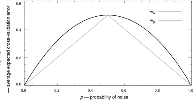
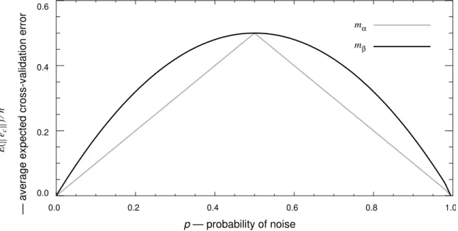
Figure 1 is a plot of as a function of p, for and . has lower expected cross-validation error than , except at the points 0, 0.5, and 1, where has the same expected cross-validation error as . When p equals 0 or 1, there is no noise in the black box, so and have the same expected cross-validation error. When p equals 0.5, the noise completely hides the deterministic component f, so again and have the same expected cross-validation error. In general, when p is neither 0, 0.5, nor 1, models that minimize error on the training set (such as ) will give sub-optimal cross-validation error.

Figure 1. Plot of as a function of p.

The next theorem shows the relation between and .

p_α p if p≤0.5 1−p ( ) if p>0.5 = p_β E e( _c )⁄n m_β p_β = 2p−2p2 E e( _c )⁄n m_α m_β m_α m_β m_α m_β m_α m_β m_α m_β m_β 0.0 0.2 0.4 0.6 0.8 1.0 0.0 0.2 0.4 0.6 m_α m_β p — probability of noise Ee c () n ⁄

— average expected cross-validation error

E( e_c )⁄n

Theorem 6:For :

(102)

Proof: When , . Therefore we have:

(103)

When , . Therefore we have:

(104)

(105) (106)

Theorem 6 shows that, for small values of p, is approximately twice the optimal . At this point, it may be worthwhile to summarize the assumptions that are made in this theory:

1. It is assumed that the inputs (the features; the attributes; the matrix X) are the same in the training set and the testing set . This assumption is the weakest ele-ment in this theory. It is discussed in detail earlier in this section and also in Section 7. It is also discussed in more depth in Turney (1993). Note that the outputs and are

not the same in the training and testing sets.

2. It is assumed that the inputs are boolean-valued. This assumption is only used in The-orem 1. The purpose of TheThe-orem 1 is to increase the credibility of the above assump-tion 1. Theorem 1 can easily be adapted to the case of multi-valued symbolic attributes. Lemma 1 covers the case of real-valued attributes. Thus there is nothing essential about the assumption that the inputs are boolean-valued.

3. It is assumed that the noise vector is a sequence of n independent random boolean variables, each having the value 1 with probability p. That is, is a sequence of sam-ples from a Bernoulli(p) distribution (Fraser, 1976). This is a very weak assumption, which is likely to be (approximately) satisfied in most real-world data (given assump-tion 6 below). 0≤ ≤p 1 p_β = 2p_α−2p_α2 0≤ ≤p 0.5 p_α = p p_β = 2p_α−2p_α2 0.5<p≤1 p_α = 1−p 2p_α−2p_α2 = 2 1( −p) −2 1( −p)2 2−2p−2+4p−2p2 = p_β = . p_β p_α X y₁ ( , ) ( , )X y₂ y₁ y₂ z z

4. It is assumed that there is noise in the class attribute (assumption 3 above), but noise in the input attributes is not addressed (due to assumption 1 above).

5. It is assumed that the data consist of a deterministic component f and a random compo-nent z. This assumption is expressed in the model . One implication of this assumption is that the target concept f does not drift with time or shift with con-text.

6. It is assumed that the output (the class attribute) is boolean-valued. The theory can easily be extended to handle multi-valued symbolic class attributes. Turney (1993) discusses real-valued outputs (and real-valued noise vectors).

With the exception of the first assumption, these assumptions are relatively weak.3 This section has presented some general results that apply to any algorithm for predict-ing boolean-valued attributes. The rest of this paper focuses on a particular class of algo-rithms: instance-based learning algorithms. This section has presented a general theory and the remainder of the paper will demonstrate that the theory can be fruitfully applied to a real, concrete machine learning algorithm.

3 Single Nearest Neighbor

Instance-based learning may be used either for predicting boolean-valued attributes (Aha

et al., 1991) or for predicting real-valued attributes (Kibler et al., 1989). Instance-based

learning is a paradigm for a class of learning algorithms; it is not a single algorithm. It is related to the nearest neighbor pattern recognition paradigm (Dasarathy, 1991).

With instance-based learning, the model is constructed by simply storing the data . These stored data are the instances. In order to make a prediction for the input , we examine the row vectors of the matrix X. In the simplest version of instance-based learning, we look for the row vector that is most similar to the input . The prediction for the output is , the element of that corresponds to the row vector .

There are many ways that one might choose to measure the similarity between two vectors. It is assumed only that we are using a reasonable measure of similarity. Let us say that a similarity measure is reasonable if:

y = f v( )⊕z y m v X y( , ) X y ( , ) v v₁,…,v_n v_i v m v X y( , ) = y_i y v_i sim u( ₁,u₂)

(107)

That is, the similarity between distinct vectors is always less than the similarity between identical vectors.

The k row vectors in X that are most similar to the input are called the k nearest

neighbors of (Dasarathy, 1991). We may use to represent instance-based learning with k nearest neighbors. This section focuses on .

The next theorem shows that instance-based learning using the single nearest neighbor gives sub-optimal cross-validation error.

Theorem 7: Let the model use instance-based learning with the single nearest neighbor. That is, if the row vector is the most similar to the input of all the row vectors of the matrix X, then . If uses a reasonable measure of similarity and no two rows in X are identical, then .

Proof: Since is based on a reasonable measure of similarity and no two rows in X are identical, no vector is more similar to than itself, so . Thus it follows from (21) that

Theorem 7 shows that satisfies the assumptions of Theorem 5. Therefore has the following properties:

(108)

(109)

In other words, is equivalent to . We know from Section 2 that gives sub-optimal cross-validation error.

If there are two (or more) identical rows in X, then (109) still holds, but (108) is not necessarily true. will, in general, no longer be equivalent to . The proof is a small variation on Theorem 5.

The problem with is that it is unstable. It is natural to consider increasing the stability of instance-based learning by considering .

u₁≠u₂→sim u( ₁,u₂)<sim u( ₁,u₁) v v m_k k = 1 m₁ m₁ v_i v v₁,…,v_n m₁(v X y, ) = y_i m₁ m₁(X X y, ) = y m₁ v_i v_i m₁(v_i X y, ) = y_i m X X y( , ) = y . m₁ m₁ E e( _t ) = 0 E e( _c ) = E e( _s ) = 2np−2np2 m₁ m_β m₁ m₁ m_β m₁ k>1

4 Voting

This section examines . Suppose the model is given the input vector . Let be the k nearest neighbors to . That is, let be the k row vectors in X that are most similar to the input vector . Let us assume a reasonable measure of similar-ity. Let be the outputs corresponding to the rows . The model predicts the output for the input to be the value of the majority of (Fix & Hodges, 1951):

(110)

Let us assume that k is an odd number, , so there will never be a tie in majority voting with . Of course, we require that . In general, .

More generally, let us consider the following model (Tomek, 1976):

(111)

In this model, t is a threshold, such that . With majority voting, . When , it may be appropriate to consider values of k other than the odd numbers.

The motivation for voting is the belief that it will increase stability; that it will make the model more resistant to noise in the data. The following sections give a formal analysis of the stability of instance-based learning with voting. They examine the best case, the worst case, and the average case.

4.1 Best Case

The next theorem concerns the best case, when stability is maximal.

Theorem 8: Let be the set of the k nearest neighbors to . Let be

k≥1 m_k v v₁, ,… v_k v v₁, ,… v_k v y₁, ,… y_k v₁, ,… v_k m_k v y₁, ,… y_k m_k(v X y, ) 0 if y_i i=1 k

∑

<k 2⁄ 1 if y_i i=1 k

∑

>k 2⁄ = k = 3 5 7, , ,… y₁, ,… y_k k≤n k«n m_k(v X y, ) 0 if y_i i=1 k

∑

<tk 1 if y_i i=1 k

∑

>tk = 0< <t 1 t = 0.5 t≠0.5 N_k( )v_i v₁, ,… v_k v_i ρ_i

defined as follows:

(112)

That is, is the frequency with which f takes the value 1, in the neighborhood of . Assume that we are using majority voting, , and that . Suppose that:

(113)

This is the most stable situation; other values of are less stable. for is deter-mined by the following formula:

(114)

In this formula, depends on . has the following values for , , , and :

(115)

(116)

(117)

(118)

Proof: Let be the k nearest neighbors to . Let be the correspond-ing elements in . Let be the corresponding elements in . The stability of

is determined by the probability that:

(119)

If we can find this probability for each row vector in X, then we can find the stability of . Suppose that is the probability of (119) when the input to is . Then is the probability that: (120) ρ_i 1 k f v( )j vj∈Nk( )vi

∑

    = i = 1, ,… n ρ_i N_k( )v_i v_i t = 0.5 k = 3 5 7, , ,… i ∀ ( ) ((ρ_i= 0) ∨ (ρ_i = 1)) ρ_i E e( _s ) m_k E e( _s ) = 2nP_k−2nP_k2 P_k m_k P_k m₁ m₃ m₅ m_∞ P₁ = p P₃ = 3p2−2p3 P₅ = 6p5−15p4+10p3 P_∞ 0 if p<0.5 0.5 if p = 0.5 1 if p>0.5 = v₁, ,… v_k v y_{1 1,} , ,… y_{1 k,} y₁ y_{2 1,} , ,… y_{2 k,} y₂ m_k y_{1 i,} i=1 k

∑

<k 2⁄ and y_{2 i,} i=1 k

∑

>k 2⁄ m_k p_i m_k v_i 2p_i m_k(v_i X y, ₁)⊕m_k(v_i X y, ₂) = 1

Therefore:

(121)

The best case — the case with minimal expected instability — arises when or . Without loss of generality, we may assume that . In this case, we have:

(122)

Therefore (119) becomes:

(123)

Let us introduce the term :

(124)

That is, is the probability that the majority of are 1, given that are all 0. The probability of (119) is:

(125)

If the best case holds for every row vector in X — that is, if (113) is true — then we have:

(126)

Let us consider the case . We have:

(127)

Recall that for we have (109):

(128)

Thus . For , we have:

(129) E e( _s ) E m( _k(v_i X y, ₁)⊕m_k(v_i X y, ₂)) i=1 n

∑

2p_i i=1 n

∑

= = E e( _s ) ρ_i = 0 ρ_i = 1 ρ_i = 0 y_{i j,} = f v( )_j ⊕z_{i j,} = 0⊕z_{i j,} = z_{i j,} i = 1 2, j = 1, ,… k z_{1 i,} i=1 k

∑

<k 2⁄ and z_{2 i,} i=1 k

∑

>k 2⁄ P_k P_k P z_{1 i,} i=1 k

∑

>k 2⁄     = P_k y_{1 1,} , ,… y_{1 k,} f v( ) …₁ , ,f v( )_k P_k(1−P_k) E e( _s ) 2P_k(1−P_k) i=1 n

∑

2nP_k(1−P_k) = = k = 3 P₃ = p3+3p2(1−p) = p3+3p2−3p3 = 3p2−2p3 k = 1 E e( _s ) = 2np−2np2 P₁ = p k = 5 P₅ = 6p5−15p4+10p3

To find the behavior of the model in the limit, , we can use the Central Limit Theorem (Fraser, 1976). Consider the following sum:

(130)

The mean and variance of this sum are:

(131)

(132)

Consider the following expression:

(133)

By the Central Limit Theorem, the distribution of (133) approaches a standard normal dis-tribution as k approaches infinity. Recall the definition of :

(134)

Let be a random variable with a standard normal distribution. As k approaches infinity, approaches: (135) We see that: (136) Therefore: m_∞ z_{1 i,} i=1 k

∑

E z_{1 i,} i=1 k

∑

    _{= kp} var z_{1 i,} i=1 k

∑

    _{= kp 1( −p)} z_{1 i,} i=1 k

∑

−kp kp 1( −p) P_k P_k P z_{1 i,} i=1 k

∑

>k 2⁄     = z_α P_k P z_α (k 2⁄ ) −kp kp 1( −p) >     k 2⁄ ( ) −kp kp 1( −p)     klim→∞ ∞ if p<0.5 0 if p= 0.5 ∞ − if p>0.5 =

(137)

(138)

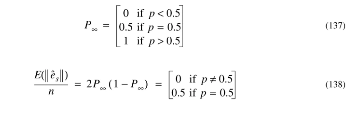
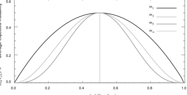
Theorem 8 implies that, in the best case, grows increasingly stable as k increases, unless . Figure 2 is a plot of as a function of p, for the models , ,

, and .

Figure 2. A plot of as a function of p.

When comparing Figure 1 with Figure 2, note that Figure 1 is a plot of , while Figure 2 is a plot of . In general, we cannot plot for , because will depend on the data. Theorems 2 and 3 show that depends on both and . The exception is , where we know that .

P_∞ 0 if p<0.5 0.5 if p = 0.5 1 if p>0.5 = E e( _s ) n 2P∞(1−P∞) 0 if p≠0.5 0.5 if p =0.5 = = . m_k p = 0.5 E e( _s )⁄n m₁ m₃ m₅ m_∞ 0.0 0.2 0.4 0.6 0.8 1.0 0.0 0.2 0.4 0.6 m₅ m₁ m₃ m_∞ p — probability of noise

— average expected instability

Ee s () n ⁄ E( e_s )⁄n E e( _c )⁄n E e( _s )⁄n E e( _c )⁄n m_k E e( _t ) E e( _c ) E e( _s ) E e( _t ) m₁ E e( _t ) = 0

(Recall that .)

Theorem 8 does not necessarily mean that we should make k as large as possible, even if we assume that the best case (113) holds. It is assumed that our goal is to minimize the expected cross-validation error. Theorems 2 and 3 show that the expected cross-validation error has two components, the error on the training set and the instability. In the best case, increasing k will increase stability, but increasing k is also likely to increase the error on the training set. We must find the value of k that best balances the conflicting demands of accuracy (low error on the training set) and stability (resistance to noise). This value will, of course, depend on f and p.

4.2 Worst Case

The next theorem concerns the worst case, when stability is minimal.

Theorem 9:Assume that we are using majority voting, , and that . Suppose that:

(139)

This is the least stable situation; other values of are more stable. for is determined by the following formula:

(140)

In this formula, depends on . has the following values for , , , and :

(141)

(142)

(143)

(144)

Proof: Let be the k nearest neighbors to . Let be the correspond-ing elements in . Let be the corresponding elements in . The stability of

m₁ = m_β t = 0.5 k = 3 5 7, , ,… i ∀ ( ) ρ_i 1 2 1 2k + = ρ_i 1 2 1 2k − = ∨ ρ_i E e( _s ) m_k E e( _s ) = 2nP_k−2nP_k2 P_k m_k P_k m₁ m₃ m₅ m_∞ P₁ = p P₃ = 2p−3p2+2p3 P₅ = 3p−9p2+16p3−15p4+6p5 P_∞ 0 if p = 0 0.5 if 0< <p 1 1 if p = 1 = v₁, ,… v_k v y_{1 1,} , ,… y_{1 k,} y₁ y_{2 1,} , ,… y_{2 k,} y₂

is determined by the probability that:

(145)

The worst case — the case with maximal expected instability — arises when:

(146)

Without loss of generality, we may assume that:

(147) (148) (149) We see that: (150) (151) Therefore: (152)

We may use the term to indicate the probability of (152). That is, is the probability that the majority of are 1, given (148) and (149). If the worst case holds for every row vector in X — that is, (139) is true — then we have:

(153)

Let us consider the case . We have:

(154) For , we have: (155) m_k y_{1 i,} i=1 k

∑

<k 2⁄ and y_{2 i,} i=1 k

∑

>k 2⁄ E e( _s ) f v( )_i i=1 k

∑

k+1 2 = or f v( )_i i=1 k

∑

k−1 2 = s k+1 2 = f v( )₁ = … = f v( )_s = 1 f v( _s+1) = … = f v( )_k = 0 y_{i j,} = ¬z_{i j,} i = 1 2, j = 1, ,… s y_{i j,} = z_{i j,} i = 1 2, j = s+ …1, ,k P y_{1 i,} i=1 k

∑

>k 2⁄     _{P z} 1 i, i=1 s

∑

z_{1 i,} i=s+1 k

∑

≤     = P_k P_k y_{1 1,} , ,… y_{1 k,} E e( _s ) 2P_k(1−P_k) i=1 n

∑

2nP_k(1−P_k) = = k = 3 P₃ = 2p−3p2+2p3 k = 5 P₅ = 3p−9p2+16p3−15p4+6p5

Again, to find the behavior of the model in the limit, we can use the Central Limit Theorem. Let and be independent random variables with a standard normal distribu-tion. As k approaches infinity, approaches:

(156)

Therefore:

(157)

(158)

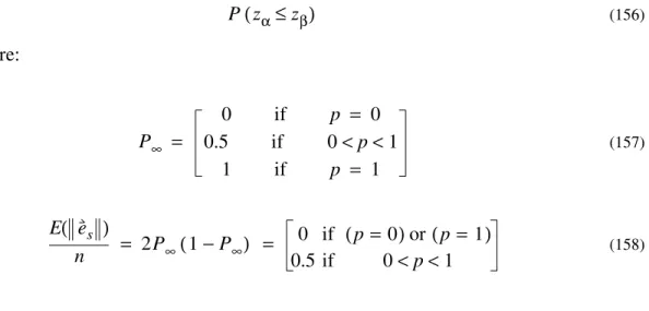
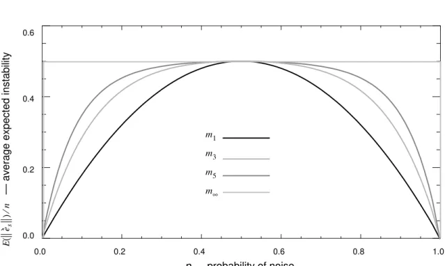
Theorem 9 implies that, in the worst case, grows increasingly unstable as k increases, unless or . Figure 3 is a plot of as a function of p, for the models

, , , and .

Figure 3. A plot of as a function of p.

m_∞ z_α z_β P_k P z( _α≤z_β) P_∞ 0 if p = 0 0.5 if 0< <p 1 1 if p = 1 = E e( _s ) n 2P∞(1−P∞) 0 if (p =0)or p( =1) 0.5 if 0< <p 1 = = . m_k p = 0 p = 1 E e( _s )⁄n m₁ m₃ m₅ m_∞ 0.0 0.2 0.4 0.6 0.8 1.0 0.0 0.2 0.4 0.6 m₅ m₁ m₃ m_∞ p — probability of noise

— average expected instability

Ee s () n ⁄ E( e_s )⁄n

4.3 Average Case

Sections 4.1 and 4.2 show that voting can be either very beneficial or very detrimental, depending on the relationship between the function f and the voting threshold t. The function f determines , the frequency with which f takes the value 1, in the neighbor-hood of . In the previous sections, we assumed majority voting, . When is near 0.5, majority voting is detrimental. When is far from 0.5, majority voting is beneficial. These results generalize to voting with other values of t. When is near t, voting is detrimental. When is far from t, voting is beneficial.

We would like to know how majority voting performs with an average f. For the average function f, is dangerously close to 0.5, or is it usually safely far away? This is a difficult question: What exactly is an average f?

The next theorem uses a simple model of an average f.

Theorem 10:Assume that we are using majority voting, . Let us suppose that we can treat as a random boolean variable, with probability that is 1, and proba-bility that is 0. In the limit, as k approaches infinity, tends to be stable, unless either or .

Proof: We see that:

(159) Recall that: (160) Therefore: (161) (162) Thus: (163) ρ_i N_k( )v_i v_i t = 0.5 ρ_i ρ_i ρ_i ρ_i ρ_i t = 0.5 f v( )_i p' f v( )_i 1−p' f v( )_i m_k p = 0.5 p' = 0.5 E f v( )_i i=1 k

∑

    _{= kp'} y_{i j,} = f v( )_j ⊕z_{i j,} i = 1 2, j = 1, ,… k P y( _{i j,} = 0) = (1−p') (1−p) +p'p P y( _{i j,} = 1) = p 1( −p') +p' 1( −p) E y_{1 i,} i=1 k

∑

    _{= k p 1[ ( −p') +p' 1( −p)] = µ}

(164)

Consider:

(165)

By the Central Limit Theorem, as k approaches infinity, (165) approaches a standard normal distribution. As before, we define as the probability:

(166)

Let be a random variable with a standard normal distribution. As k approaches infinity, approaches: (167) We see that: (168) Therefore: (169) (170)

Thus tends to be stable, unless:

(171) var y_{1 i,} i=1 k

∑

    _{= k p 1[ ( −p') +p' 1( −p)] [(1−p') (1−p) +p'p] = σ}2 y_{1 i,} i=1 k

∑

−µ σ P_k P y_{1 i,} i=1 k

∑

>k 2⁄     z_α P_k P z( _α> ((k 2⁄ ) µ− ) σ⁄ ) k 2⁄ ( ) µ− ( ) σ⁄ ( ) klim→∞ ∞ if [p 1( −p') +p' 1( −p)] <0.5 0 if [p 1( −p') +p' 1( −p)] = 0.5 ∞ − if [p 1( −p') +p' 1( −p)] >0.5 = P_∞ 0 if [p 1( −p') +p' 1( −p)] <0.5 0.5 if [p 1( −p') +p' 1( −p)] = 0.5 1 if [p 1( −p') +p' 1( −p)] >0.5 = E e( _s ) n 2P∞(1−P∞) 0 if [p 1( −p') +p' 1( −p)] ≠0.5 0.5 if [p 1( −p') +p' 1( −p)] = 0.5 = = m_k p 1( −p') +p' 1( −p) = 0.5

Some algebraic manipulation converts (171) to:

(172)

Therefore tends to be stable, unless either or

Let us now consider the general case (111), when the threshold for voting t is not nec-essarily equal to 0.5.

Theorem 11:Let t be any value, such that . Let us suppose that we can treat as a random boolean variable, with probability that is 1, and probability that

is 0. Let us introduce the term :

(173)

In the limit, as k approaches infinity, tends to be stable, unless .

Proof: This is a straightforward extension of the reasoning in Theorem 10

Presumably p (the probability that z is 1) and (the probability that f is 1) are not under the control of the modeler. However, t can be adjusted by the modeler. If the modeler can estimate p and , then can be estimated. Theorem 11 implies that the modeler should make sure that t is relatively far from .

The assumption that we can treat as a random boolean variable is somewhat unre-alistic. Let us consider a more sophisticated analysis.

Theorem 12:Let us define as follows:

(174)

In the limit, as k approaches infinity, tends to be stable for , unless t is close to .

Proof: This is a straightforward extension of the reasoning in Theorem 10

Let us define as the average of the :

(175) Note that: 2p−1 ( ) (1−2p') = 0 m_k p = 0.5 p' = 0.5 . 0< <t 1 f v( )_i p' f v( )_i 1−p' f v( )_i τ τ = p 1( −p') +p' 1( −p) = p+p'−2pp' m_k t = τ . p' p' τ τ f v( )_i τ_i τ_i = p+ρ_i−2pρ_i i = 1, ,… n m_k v_i τ_i . p' ρ_i p' 1 n ρi i=1 n

∑

=

(176)

We can use (173) and (175) to calculate . Theorem 12 implies that it is possible for to be stable even when , if t is far from each .

Theorem 13:We can estimate from the data as follows:

(177)

is an unbiased estimator for .

Proof: We have:

(178)

(179)

(180) (181)

Using (177), we can estimate for any k and any i. is the frequency of the output 1, in the neighborhood of .

Theorem 14: If we know the value of p, then we can also estimate from the data :

(182)

is an unbiased estimator for .

Proof: We have: p' 1 n f v( )i i=1 n

∑

≠ τ m_k t = τ τ_i τ_i ( , )X y₁ t_i 1 k y1 j, vj∈Nk( )vi

∑

    = i = 1, ,… n t_i τ_i E t( )_i 1 k E y( 1 j, ) vj∈Nk( )vi

∑

    = 1 k E f v(( )j ⊕z1 j, ) vj∈Nk( )vi

∑

    = p+ρ_i−2pρ_i = τ_i = . τ_i t_i N_k( )v_i v_i ρ_i X y₁ ( , ) r_i ti−p 1−2p = r_i ρ_i

(183)

(184) (185) (186)

Using (177) and (182), we can estimate for any k and any i. Once we have an estimate of , we can establish whether we are closer to the best case (Section 4.1) or the worst case (Section 4.2).

We now have some understanding of the average behavior of in the limit. Let us consider the average behavior of for and .

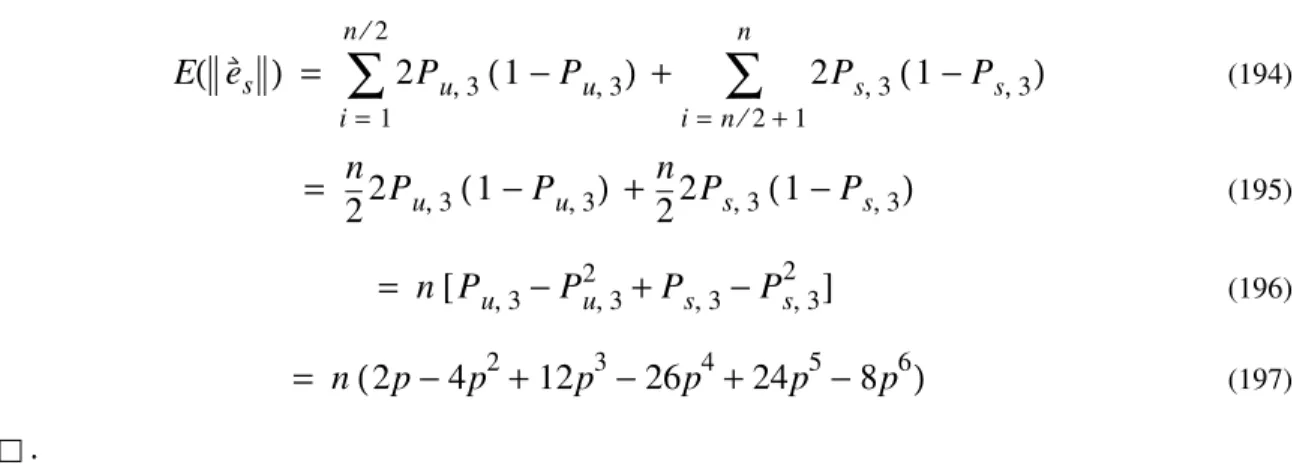
Theorem 15:Suppose that n is even. Let and . Suppose that:

(187) (188)

Then:

(189)

Proof: We know from Section 4.2 that is unstable when:

(190)

We know from Section 4.1 that is stable when:

(191)

For the unstable case, , we have (154):

(192)

For the stable case, , we have (127):

(193) Therefore (126): E r( )_i E t( )i −p 1−2p = τ_i−p ( ) ⁄ (1−2p) = p+ρ_i−2pρ_i−p ( ) ⁄ (1−2p) = ρ_i = . ρ_i ρ_i m_k m_k k = 3 t = 0.5 k = 3 t = 0.5 ρ_i = 1 3⁄ or ρ_i = 2 3⁄ i = 1, ,… n 2⁄ ρ_i = 0 3⁄ or ρ i = 3 3⁄ i = n 2⁄ + …1, ,n E e( _s ) = n 2p( −4p2+12p3−26p4+24p5−8p6) m₃ ρ_i = 1 3⁄ or ρ_i = 2 3⁄ i = 1, ,… n m₃ ρ_i = 0 3⁄ or ρ_i = 3 3⁄ i = 1, ,… n i = 1, ,… n 2⁄ P_{u 3,} = 2p−3p2+2p3 i = n 2⁄ + …1, ,n P_{s 3,} = 3p2−2p3

(194)

(195)

(196)

(197)

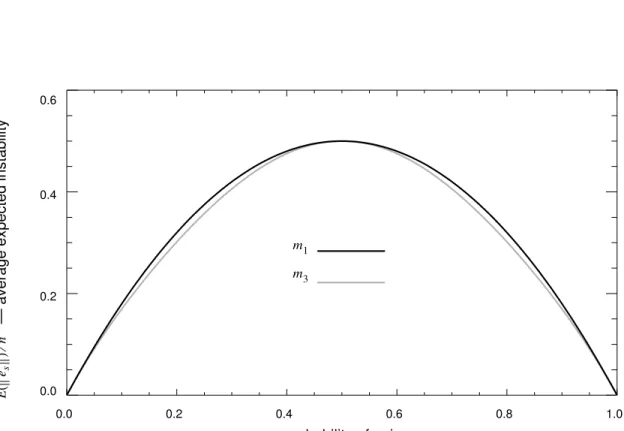
Figure 4 is a plot of for , using the average case analysis of Theorem 15. For comparison, is also plotted for . is slightly more stable than , except at 0, 0.5, and 1, where they are equal.

Figure 4. A plot of as a function of p.

5 Application

Let us assume that n, p, X, and are fixed, while k and t are under our control. Our goal is to minimize the expected cross-validation error. The data X and are the training set, and the testing set is not yet available to us. How do we determine the best values for k and t?

E e( _s ) 2P_{u 3,} (1−P_{u 3,} ) i=1 n 2⁄

∑

2P_{s 3,} (1−P_{s 3,} ) i=n 2⁄ +1 n

∑

+ = n 22Pu 3, (1−Pu 3, ) n 22Ps 3, (1−Ps 3, ) + = n P[ _{u 3,} −P_{u 3}2_, +P_{s 3,} −P_{s 3}2_, ] = n 2p( −4p2+12p3−26p4+24p5−8p6) = . E e( _s )⁄n m₃ E e( _s )⁄n m₁ m₃ m₁ 0.0 0.2 0.4 0.6 0.8 1.0 0.0 0.2 0.4 0.6 m₁ m₃

— average expected instability

Ee s () n ⁄ p — probability of noise E( e_s )⁄n y y