A case study of sever selection

A Case Study of Server Selection

by

Tina Tyan

S.B., Computer Science and Engineering (2000)

Massachusetts Institute of Technology

Submitted to the Department of Electrical Engineering and Computer Science

in partial fulfillment of the requirements for the degree of

Master of Engineering in Electrical Engineering and Computer Science

at the

MASSACHUSETTS INSTITUTE OF TECHNOLOGY

September 2001

©

Massachusetts Institute of Technology 2001. All rights reserved.

Author ...

Department of Electrical Engineering and Computer Science

August 8, 2001

C ertified by ...

M. Frans Kaashoek

Professor of omputer Science and Engineering

Thesis Supervisor

Accepted by ... ... . .

Arthur C. Smith

Chairman, Department Committee on Graduate Theses

BARK

L

OF TECHNOLOGY

A Case Study of Server Selection

by Tina Tyan

Submitted to the Department of Electrical Engineering and Computer Science on August 8, 2001, in partial fulfillment of the

requirements for the degree of

Master of Engineering in Electrical Engineering and Computer Science

Abstract

Replication is a commonly used technique to improve availability and performance in a distributed system. Server selection takes advantage of the replicas to improve the end-to-end performance seen by users of the system. CFS is a distributed, cooperative file system that inherently replicates each piece of data and spreads it to machines dispersed around the network. It provides mechanisms for both locating and retrieving data. This thesis considers the application of server selection to improving performance in CFS, in both the data location and data retrieval steps. Various server selection metrics and methods were tested in an Internet testbed of 10-15 hosts to evaluate the relative benefits and costs of each method.

For the lookup step, we find that the triangle inequality holds with good enough corre-lation that past latency data stored on intermediary nodes can be used to select each server along the lookup path and reduce overall latency. For the data retrieval step, we find that selecting based on an initial ping probe significantly improves performance over random selection, and is only somewhat worse than issuing parallel requests to every replica and taking the first to respond. We also find that it may be possible to use past latency data for data retrieval.

Thesis Supervisor: M. Frans Kaashoek

Acknowledgments

Several of the figures and graphs in this thesis, as well as the pseudocode, came from the SIGCOMM[24] and SOSP[8] papers on Chord and CFS. There are a number of people who have helped me through the past year and who helped make this thesis possible. I'd like to thank Kevin Fu for his help getting me started, and Frank Dabek for his help on the later work. Thank you to Robert Morris for his invaluable feedback and assistance. I would also like to thank the other members of PDOS for their suggestions and ideas. I would especially like to thank my advisor, Frans Kaashoek, for his guidance, patience, and understanding. Thanks also to Roger Hu for always being available to answer my questions (and for all the free food), and Emily Chang for her support and assistance in getting my thesis in shape (particularly the Latex). Working on a thesis isn't just in the work, and so I'd like to extend my appreciation to the residents of the "downstairs apartment", past and present, for giving me a place to get away from it all, especially Danny Lai, Stefanie Chiou, Henry Wong, Roger, and Emily. A special thanks to Scott Smith, for always being there for me, whether with suggestions, help, or just an ear to listen. Lastly, I'd like to thank my family

-Mom, Dad, Jeannie, and Karena -for all their support and love. I would never have gotten

Contents

3.1.1 Past Latency Data . . . . 25

3.1.2 Triangle Inequality . . . . 26

3.2 Selection at the dhash layer . . . . 26

3.2.1 Random Selection . . . . 27 3.2.2 Past Performance. . . . . 27 3.2.3 Probing . . . . 28 3.2.4 Parallel Retrieval . . . . 29 4 Experiments 31 4.1 Experimental Conditions. . . . . 31

4.2 Chord Layer Tests . . . . 32

4.2.1 Evaluating the use of past latency data . . . . 32

4.2.2 Triangle Inequality . . . . 36

4.2.3 Chord Layer Selection Results . . . . 43

4.3 dhash Layer Tests . . . . 44

4.3.2 4.3.3 4.3.4 4.3.5

Ping Correlation Test . . . . Selection Tests . . . .

Parallel Downloading Tests - Methodology .

Combined Tests . . . .

5 Related Work

5.1 Internet Server Selection . . . .

5.1.1 Intermediate-level Selection . . . . 5.1.2 Client-side. . . . . 5.2 Peer-to-peer Systems . . . . 6 Conclusion 6.1 Conclusion . . . . 6.2 Future Work . . . .. . . . . . . . . 4 5 . . . . 4 9 . . . . 5 0 . . . . 5 1 57 . . . . 5 7 . . . . 5 8 . . . . 6 1 . . . . 6 5 69 69 70

List of Figures

2-1 2-2

2-3

Example Chord ring with 3 nodes. . . . . Example Chord Ring with Finger Tables . . . . The pseudocode to find the successor node of an identifier id. Remote pro-cedure calls and variable lookups are preceded by the remote node.

2-4 CFS Software Layers . . . .

3-1 Example of choice in lookup algorithm . . . .

4-1 RON hosts and their characteristics . . . .

4-2 Sightpath to Msanders Ping Times . . . .

4-3 Cornell to Sightpath Ping Times . . . .

4-4 Mazu to Nc Ping Times . . . .

4-5 nc to lulea Ping Times . . . .

4-6 Simple Triangle Inequality . . . .

4-7 Triangle Inequality: AC vs AB+BC . . . .

4-8 Relative Closeness . . . .

4-9 Chain of Length 3 . . . .

4-10 Best and Worst Ping Ratios for Tests 1 and 2 . . . . 4-11 Best Ping Ratio for Tests 1 and 2 (same as in figure 4-10) 4-12 Best and Worst Ping Ratios for Test 3 . . . . 4-13 Best Ping Ratio for Test 3 (same as in figure 4-12) . . . .

4-14 Parallel Retrieval Results . . . . 4-15 Ping Probe Results . . . . 4-16 Aros Ping Probe Results . . . . 4-17 Random, Best Ping, Parallel Results . . . .

17 19 20 21 25 . . . . 32 . . . . 34 . . . . 35 . . . . 35 . . . . 36 . . . . 37 . . . . 38 . . . . 39 . . . . 41 . . . . 47 . . . . 47 . . . . 48 . . . . 48 . . . . 53 . . . . 54 . . . . 54 . . . . 56

Chapter 1

Introduction

The Internet is becoming an ubiquitous part of life as increasingly large numbers of people are going online and the number of available resources grows. Users use the Internet to ob-tain all types of public data, from web pages to software distributions. However, along with increased popularity and usage come problems of scalability and performance degradation. When a popular resource is only available from a single source, that server can experience excessive load, to the point of being unable to accommodate all requests. Users located geographically or topologically far from the server are prone to excessive latency, which can also be caused by network bottlenecks or congestion. This sole source also provides a single point of failure; if this server goes down, then the resource becomes completely unavailable. Server replication provides a viable solution to many of these problems, improving per-formance and availability. In replication, some subset of the server's data or a given resource is duplicated on multiple servers around the network. The existence of replicas allows re-quests for data to be distributed, lessening the load on each server and accommodating greater overall load. Replicas also add redundancy to the system; if one server goes down, there are still many others available to take up the slack. If the replicas are distributed across the network, then a given client has a greater chance of being located closer to a source of the data, and therefore experiencing lower latency than if it tried to contact one central server.

Along with replication comes the added problem of server selection. In order for repli-cated services to be useful, a replica must be selected and assigned to a client by some method. This selection can be done by the server, by the client, or by some intermediary

service. The criteria and method of selection will have varying impacts on performance and server load. It is in this step that the real benefits of replication are derived. The interesting thing about server selection is that there is no easy way to choose the best server; varying network conditions, server load, and other factors can change performance characteristics from client to client and request to request. Additionally, what is considered to be "best" varies from system to system.

This thesis considers the specific problem of server selection within CFS (Cooperative File System), a distributed, decentralized file system designed to allow users to coopera-tively pool together available disk space and network bandwidth. CFS has many useful properties that make it an attractive system to use, and could benefit from improved per-formance. An important feature of CFS is its location protocol, which is used to locate data in the system in a decentralized fashion. CFS inherently takes care of replication, replica management, and replica location, three primary concerns in any replicated system. Although the basic motivation behind replication is the same as in other systems, CFS has specific requirements and characteristics that make it somewhat unique from other systems in which server selection has been studied.

CFS' decentralized, cooperative nature means that instead of having a dedicated set of

servers and replicas with distinct clients that access them, every node in the system can act as both a client and a server. Also, the location protocol of CFS, to be described in greater detail in chapter 2, utilizes nodes to act as intermediaries in the lookup process. Therefore nodes acting as servers are constantly in use for purposes other than serving data, and do not have to be particularly high performance machines behind high bandwidth links. CFS also ensures that data is replicated on machines that are scattered throughout the Internet. The pool of servers for a particular piece of data is therefore quite diverse, and certain servers are likely to have better performance for a given client than others. Additionally, while Web-based systems must deal with files of all sizes, CFS uses a block-level store, dividing each file into fixed size blocks that are individually retrieved. These block sizes are known and can be taken advantage of in choosing a server selection mechanism, whereas the sizes of Web files are not known before retrieval, making any size-dependent mechanism hard to use. Storing data at the level of blocks also load balances the system, so that the selection method need not be particularly concerned with keeping the load balanced.

performance experienced by the client. For CFS, this does not only include the end-to-end performance of the data retrieval from a replica, but also includes the overall performance of the data location step. The requirements for selection for location are fairly distinct from those of data retrieval. The purpose of this thesis is to investigate and experimentally eval-uate various server selection techniques for each stage of CFS operation, with the intention of improving overall end-to-end performance in the system.

Chapter 2 will give a brief overview of CFS and how it works. Chapter 3 goes into more detail on the requirements for selection in CFS, as well as those aspects of the system most directly relevant to server selection. Chapter 4 describes the experiments conducted to evaluate the selection techniques introduced in the previous selection, as well as the results so obtained. Previous work done in server selection, both for the World Wide Web

and other peer-to-peer systems, is described in chapter 5. Lastly, chapter 6 wraps up the discussion and proposes future directions for work in this area.

Chapter 2

Background

This thesis studies server selection techniques and conditions in the context of the Chord/CFS system. To better understand the problems that server selection must address, we take a closer look at the system in question in this chapter. The next chapter will discuss server selection within Chord and CFS and highlight relevant aspects of the system.

2.1

Overview

In recent years, peer-to-peer systems have become an increasingly popular way for users to come together and share publicly-accessible data. Rather than being confined to the disk space and bandwidth capacity available from a single (or even several) dedicated server(s), the peer-to-peer architecture offers the ability to pull together and utilize the resources of a

multitude of Internet hosts (aka nodes). As a simple example, if the system was comprised of

1000 nodes with only 1MB free disk space on each, the combined disk capacity of the entire

system would total 1GB. Participating nodes are likely to contribute far more than 1MB to the system. Given more hosts and more available disk space, the potential available storage in such a system far exceeds that of a traditional client-server based system. Similarly, the potential diversity of the available data is increased by the fact that there can be as many publishers of data as there are users of the system. At the same time, since there is no single source of information, the bandwidth usage is distributed throughout the system.

Although the concept of the peer-to-peer architecture is attractive, implementing such a system offers some challenges. Recent systems like Napster and Gnutella have received widespread use, but each has its limitations. Napster is hampered by its use of centralized

servers to index its content[16]. Gnutella is not very scalable since it multicasts its queries

[11]. Other peer-to-peer systems experience similar problems in performance, scalability,

and availability [24]. One of the biggest challenges facing these systems is the problem of efficiently and reliably locating information in a decentralized way. CFS (Cooperative File System) is a cooperative file system designed to address this problem in a decentralized, distributed fashion. It is closely integrated with Chord, a scalable peer-to-peer lookup protocol that allows users to more easily find and distribute data. We give a brief overview

of Chord and CFS in this chapter; details can be found in [7], [8], [24], and[25].

2.1.1 Chord

Chord provides a simple interface with one operation: given a key, it will map that key onto a node. Chord does not store keys or data itself, and instead acts as a framework on top of which higher layer software like CFS can be built. This simple interface has some useful properties that make it attractive for use in such systems. The primitive is efficient, both in the number of machines that need to be contacted to locate a given piece of data, and in the amount of state information each node needs to maintain. Furthermore, Chord adapts efficiently when nodes join or leave the system, and is scalable with respect to the total number of participating nodes in the system.

2.1.1.1 Chord Identifiers

Each node in the Chord system is associated with a unique m-bit Chord node identifier, obtained by hashing the node's IP address using a base hash function, such as SHA-1. Just as nodes are given node identifiers, keys are also hashed into m-bit key identifiers. These

identifiers, both node and key, occupy a circular identifier space modulo ₂m. Chord uses

a variant of consistent hashing to map keys onto nodes. In consistent hashing, the node responsible for a given key k is the first node whose identifier is equal to or follows k's identifier in the identifier space. When the identifiers are pictorially represented as a circle of numbers from 0 to 2m - 1, this corresponds to the first node clockwise from k. This node

is known as the "successor" of k, or successor(k).

A simple example of a Chord network for which m=3 is seen in Figure 2-1. There are

three nodes in this network, with identifiers 0, 1, and 3. The set of keys' identifiers to be stored in this network is {1, 2, 6}. Within this network, the successor of key 1 is node 1,

7 1 successor(1)= 1

successor(6)=0 6 2 successo(2)=3

5 3

4 2

Figure 2-1: Example Chord ring with 3 nodes

since the identifiers match. The successor of key 2 is node 3, which can be found by moving clockwise along the circle to the next node after 2. Similarly, the successor for key 6 is the first node found clockwise after 6 on the identifier circle, which in this case wraps around to node 0.

2.1.1.2 Consistent Hashing

There are several benefits to using consistent hashing. Consistent hashing allows nodes to join and leave the network with minimal disruption. When a node joins the network, a certain set of keys that previously mapped to its successor are reassigned to that node. In the above example, if node 7 were to join the network, key 6 would be reassigned to it instead of node 0. Similarly, when a node leaves the network, its keys are reassigned to its successor. In this way, the consistent hashing mapping is preserved, and only a

minimal number of keys - those for the node in question - need to be moved. Consistent

hashing also provides load balancing, distributing keys with high probability in roughly equal proportions to each node in the network.

In a centralized environment where all machines are known, consistent hashing is straight-forward to implement, requiring only constant time operations. However, a centralized sys-tem like that does not scale. Instead, Chord utilizes a distributed hash function, requiring each node to maintain a small amount of routing information.

2.1.1.3 Key Location

In order for consistent hashing to work in a distributed environment, the minimum amount of routing information needed is for each node to be aware of its successor node. A query for a given identifier k would therefore follow these successor pointers around the circle until the successor of k was found. This method is inefficient, however, and could require the query to traverse all N nodes before it finds the desired node. Instead, Chord has each node maintain a routing table of m entries (corresponding to the m-bit identifiers), called the finger table.

The finger table is set up so that each entry of the table is "responsible" for a particular segment of the identifier space. This is accomplished by populating each entry i of a given

node n with the Chord ID and IP address of the node s = successor(n + 2i-mod2"),

where 1 < i < m. This node, s, is also known as the ith finger of n, and is denoted as n.finger[i].node. Thus, the 1st finger of n is its immediate successor (successor(n + 1)), and each subsequent finger is farther and farther away in the identifier space. A given node therefore has more information about the nodes nearest itself in the identifier space, and less information about "far" nodes. Also stored in the ith entry of the finger table is the jth finger interval. This is fairly straightforward; since the ith finger is the successor of (n + 2i-) and the i + 1th finger is the successor of (n+ 2i), then n.finger[i].node is this node's predecessor

for any identifier that falls within the interval [n.finger[i].node, n.finger[i+1].node). Figure 2-2 shows the finger tables for the simple Chord ring examined earlier. Since m

= _{3, there are 3 entries for each finger table. The finger table for node 1 is populated with}

the successor nodes of the identifiers (1 + 21-1) mod 23 = 2, (1 + 22-1) mod 23 = 3 and

(1 + 231) mod 23 = 5. In this particular network, successor(2) = 3, successor(3) = 3, and

successor(5) = 0. The finger tables for the other nodes follow accordingly.

These finger tables allow Chord to systematically and efficiently search for the desired node by directing queries increasingly closer in the identifier space to that node. The closer a node is to a region of the identifier circle, the more it knows about that region. When a node n does not know the successor of a key k, it looks in its finger table for the set of nodes between itself and the destination in ID space. These nodes are all closer in ID space to the key than the origin, and are possible candidates to ask for its location. The simplest implementation chooses the node n' closest in ID space to k and sends it a

closest-preceding-finger table keys start int.

odode

[

1 [1,2) 1

2 ,4 finger table keys

4 [4,0) 0 start int. ode

2 [2,3 3 3 [3,5,3 S5 [5,l) 0 7 1 6 2 5 3

finger table keys

4 start int. node 4 [4,5)

7 [7,3) 0

Figure 2-2: Example Chord Ring with Finger Tables

nodes RPC. Node n' then looks in its finger table and sends back the list of successors between itself and the destination, allowing n to select the next node to query. As this process repeats, n learns about nodes with IDs closer and closer to the target ID. The process completes when k's predecessor is found, since the successor of that node is also k's successor. The pseudocode for these procedures can be found in figure 2-3.

A simple Chord lookup query takes multiple hops around the identifier circle, with each

hop eliminating at least half the distance to the target. Consequently, assuming node and key identifiers are random, the typical number of hops it takes to find the successor of a given key is O(log N), where N is the number of nodes in the network. In order to ensure proper routing, even in the event of failure, each node also maintains a "successor-list" of its r nearest successors on the Chord ring. In the event that a node notices its successor has failed, it can direct queries to the next successor in the "successor-list," thus updating its successor pointer.

The Chord protocol also has provisions for initializing new nodes, and for dealing with nodes concurrently joining or leaving the network. These aspects of the protocol are not relevant to server selection, and are not necessary to understand the system.

// ask node n to find id's successor

n.find-successor(id)

n' = (id);

return n'.;

//

n.find-predecessor(id) n' =

n;

/7

7/

n.closest-preceding-nodes(id)

return {n' E {fingers U successors}

s.t. n' e (n,id)}

Figure 2-3: The pseudocode to find the successor node of an identifier id. Remote procedure calls and variable lookups are preceded by the remote node.

2.1.2 CFS

Chord was created as a general-purpose location protocol, with the intention that higher-level systems with more specific functionality would be built on top of it. One such system is CFS, a read-only file system designed to allow users to cooperatively pool disk space and network bandwidth in a decentralized, distributed fashion. CFS nodes cooperate to locate and load-balance the storage and serving of data in the system. CFS consists of three layers (Figure 2-4): the file system layer, which provides the user with an ordinary file system interface; the dhash layer, which takes care of data storage and retrieval issues; and the Chord layer, which provides mappings of keys and nodes, and acts as a location service. Data is not stored at the level of full files, but instead as uninterpreted blocks of data with unique identifiers. The client may interpret these blocks as file data or as file system metadata.

2.1.2.1 dhash layer

For the purposes of server selection, the relevant functions of CFS occur at the dhash layer. The way that blocks are assigned to servers is very closely tied to the way the underlying

FS

DHash DHash DHash

Chord Chord Chord

CFS Client CFS Server CFS Server

Figure 2-4: CFS Software Layers

Chord protocol functions. Each block of data has an associated unique identifier. This ID could be a cryptographic hash of the block's contents or a public key, and is equivalent to a key in Chord. A block is stored at the server that Chord identifies as the successor of the block's key.

There are some tradeoffs to keeping everything at the block level and storing the data in this way. Blocks are distributed roughly evenly around the ID space, since the hash function uniformly distributes the block IDs. Consequently, the data is not all retrieved through the same paths and bandwidth usage is spread around the network. This provides the system with a certain degree of load balancing. However, instead of doing one Chord lookup per file or file system accessed, this system requires there to be one Chord lookup per block retrieved, reducing location and retrieval efficiency.

2.1.2.2 Replication

CFS takes advantage of other properties of Chord to increase availability and potentially

increase efficiency through replication. As part of its failure recovery mechanism, each Chord node maintains a "successor-list" of its nearest r successors on the Chord ring, which is automatically updated and maintained as nodes come and go. These successors are a natural place to replicate the data. There are two main concerns for replicated data: keeping track of the replicas so that the data can be found and updated, and making sure the replicas are independent of failure, so that if one machine goes down, the replica will still be available. The node is already keeping track of the r successors through its successor

list, so there is no need for an external mechanism to maintain the replicas. At the same time, these successors are unlikely to be near each other geographically or topologically, since their Chord IDs are hashes of their IP addresses. Numerically similar addresses are unlikely to hash to numerically similar identifiers, by the nature of the hash function. This means that the replicas are more likely to be failure independent and also that it is likely that at least one of the replicas will be close to a given client.

Aside from providing higher availability, this replication scheme paves the way for per-formance improvements through server selection, as will be described in greater detail in the following chapter.

Chapter 3

Server Selection in CFS

The current implementation of CFS does not do any sort of server selection, and instead just uses the first server found to contain the desired block. Performance tests run on a collection of 8 CFS servers spread over the Internet indicates that performance is strongly affected by the characteristics of the particular servers involved. When a server was added which happened to be far from the client, transfer times increased dramatically, while nearby servers helped to decrease transfer time. Although some of the effects of this can be alleviated through the use of pre-fetching (requesting several blocks simultaneously), these tests indicate a strong need for server selection to reduce variation in and improve the performance of the system.

There are two particular points in the CFS system where server selection could come into play. The first is at the Chord level, during the location protocol, while the second is at the dhash layer, in the actual data retrieval step. The nature of the selection required is somewhat different at these two layers, and leads to different requirements for a selection method.

3.1

Server Selection at the Chord layer

Server selection in the lookup layer strives to reduce the overall latency and variation in lookup times by eliminating as much as possible the need to make large geographical leaps in the lookup process. The CFS implementation of the Chord protocol facilitates the use of server selection by naturally providing a list of alternative nodes at each stage of the lookup process.

When a lookup is performed, the origin node n tries to find the predecessor of the desired key k by issuing a closest-preceding-nodes RPC to a node n' in its finger table that is closer in ID space to k than n is. Node n'subsequently looks in its own finger table and returns a group of successors that are all closer in ID space to k. This process is reiterated until the

desired successor is found. In the current implementation, the node in this list of successors with the ID closest to k is the one selected for the next step of the implementation. While this method keeps the number of necessary hops around the Chord ring to a minimum since it makes the largest advances in ID space towards the target, the overall lookup time is strongly dependent on the performance of each intermediate node. If even one intermediate

node thus chosen is particularly slow - in a different country, for instance - then the

overall lookup time is significantly impacted. Potentially, server selection could be used at each stage of the lookup process to keep each query local, resulting in perhaps more hops but lower overall latency.

The developers of Chord and CFS are currently investigating an alternate lookup algo-rithm that would utilize server selection in a different way. Instead of simply picking the node with the closest ID, this algorithm examines all the possible servers in the finger table and selects the one that is most likely to keep the overall latency minimal. This is deter-mined through a combination of factors. At each step of the lookup process, the algorithm strives to get closer to the destination ID through bit correction of the IDs -picking servers whose IDs match increasingly more bits of the destination ID. The number of future hops needed to arrive at the destination from that node can therefore be estimated by looking at the amount of bit correction needed on that node's ID. At the same time, CFS keeps track of the costs of all RPC's in the system, and can use this to estimate the average hop latency.

By using a combination of these two estimates, and factoring in the latency between the

selecting node and the potential intermediate node, the client can choose the intermediate node with the lowest potential cost/highest potential gain for the next step of the lookup.

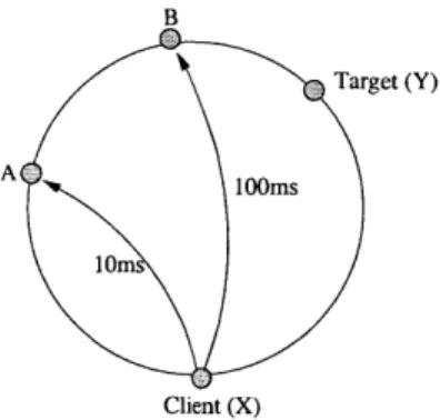
Figure 3-1 gives a simple example to explain how this algorithm works. Nodes A and B are on the identifier ring between the client X and the target Y. B is closer to the target in ID space, and has a latency from the client of 100ms, while A is farther and has a latency of 10ms. As CFS runs, it keeps track of all previous transactions, and can determine the average latency of a hop based on this information. The client can also estimate the number of hops remaining between a given node and the target, based on the ID. Using these two

B

Target (Y)

A _looms

lOm

Client (X)

Figure 3-1: Example of choice in lookup algorithm

pieces of information, the client can then make a comparison between nodes A and B. If

HopLatency * NumHopsAy + LatencyxA < HopLatency * NumHopSBY + LatencyXB

then it may be better to pick node A rather than B. This is also another application of the triangle equality, with A and B acting as the intermediary nodes. If X-A-Y is not less than X-B-Y, then the whole thing falls apart.

The goals of server selection, and therefore the relevant metrics, can change depending on its overall purpose. In this case, the purpose of selection is not to find the server that will return data the fastest, but instead the server that responds fastest to a small lookup query. Therefore, round-trip latency should be a good indicator. However, it is not just a straightforward matter of always picking the successor with the lowest latency. There are a number of issues to be resolved in order to choose an appropriate selection method, and to determine if selection is even viable at all in reducing the overall latency of the lookup process.

3.1.1 Past Latency Data

Unlike with large downloads, where the time to probe the machines before selection is insignificant in comparison to the download time, each lookup hop only imposes a small overhead on top of the time to reach the machine. This overhead includes transmitting the request, searching the finger table, and returning the list of successors. Therefore, the time it would take to make just one round trip to the machine to probe it would impose a significant overhead on the overall time. Selection would be useful only if it could be done

solely on the basis of past latency data. If latency between machines varies widely over time, then past latency data may be insufficient to select the fastest machine.

Even assuming that the fastest machine can be found using past latency data, it is not clear that this will necessarily lead to better overall lookup latency. For every step of the lookup process except the initial request, the client chooses from a list of successors given to it by another node. The client does not maintain any past metrics for these machines and can rely only on the other node's information. Therefore, the available past performance data is not directly relevant to the client doing the selection, and it is impractical to probe the nodes before selecting one. If it could be shown that this indirect information is sufficient to improving the overall performance, then it will be possible to devise a good server selection method for the Chord layer.

3.1.2 Triangle Inequality

The specific question at hand is whether knowing which machine is closer to an intermediate machine is correlated to knowing which is closest to the client. A basic expression of this is the triangle inequality, which seeks to determine if machine A is close to machine B, and machine B is close to machine C, does it necessarily follow that machine A is close to machine C? More relevantly, if B is closer to X than Y, will A also be closer to X than Y? Since an actual lookup is likely to take several steps, it may also be useful to examine chains of such comparisons to see if utilizing the same methods through several levels of indirection still yields similar answers. If this is true, then always picking the fastest machine in each step of the lookup process will succeed in keeping the lookup process as topologically close to the client as possible, thus reducing the overall latency. If this isn't true, then latency won't help in deciding which machine to choose.

3.2

Selection at the dhash layer

After the lookup process is completed, and the key's successor is known, the client has the necessary information to download the desired block. It can choose to download from the actual successor, or to utilize the replicas on the following k successors in some sort of server selection scheme. The main goal of such a selection scheme would be to improve end-to-end performance.

3.2.1

Random Selection

The simplest selection method would be to randomly select a node from the list of replicas to retrieve the data from. This method incurs no additional overhead in selection, and has the effect of potentially distributing the load to these replicas if the block is popular. Although the random method has as good a chance of picking a slow server as a fast one, with each subsequent request it will likely pick a different server and not get stuck on the slow one. Without selection at all, if the successor of the key is slow, then all requests will be limited by the response time of this particular node.

3.2.2 Past Performance

Alternatively, selection could be done on the basis of past performance data. Clients can make an informed decision using past observed behavior to predict future performance. Previously, systems using past performance as their metric made use of a performance database, stored either at the client or at some intermediate resolver. This performance database included information on all known replicas for a previously accessed server. In a Web-based system with a few servers and many clients, this method is quite manageable. However, keeping such a performance database is less viable within CFS. The database is only useful if a client is likely to revisit a server. When a client has no knowledge of a particular set of replicas, it can not use past data to perform selection and must use some other form of selection for that initial retrieval. Even if it has accessed this data before, if the access did not take place recently, the performance data may no longer be relevant because of changes in the network. Thus the performance database must be kept up to date. With the potentially large number of nodes in a Chord network, and the way that blocks are distributed around the network, it does not seem likely that the same client will retrieve blocks from the same server with any great frequency. Therefore, it will constantly be encountering servers for which it has no information, while its stored performance data for other servers is rarely used and rapidly goes out of date.

However, past performance can still be used as the basis of server selection in CFS, without the need for a performance database. The method would in fact be very similar to that used in the Chord layer. Each node in the CFS system keeps in regular contact with its fingers and successors in order to keep its finger table and successor-list up to date.

The node therefore already stores fairly up-to-date latency information for each of these servers. Since the replicas for this node are located in the successors to the node, the node has past latency information for each replica. Using this information will require no extra trips across the network or additional overhead. Each lookup ends at the predecessor to the desired node, and its successor list will include all the replicas and their corresponding latency data. When the lookup returns the list of replicas to the client, the client can just use this information to select a server, much as it does for each stage of the lookup. A few crucial assumptions must be true for this method to work well. Since the nodes store past latencies, and not end-to-end performance data, latency must be a good indicator for end-to-end performance. The current block size in CFS is 8KB, which is adequately small enough that this is likely to be true. At the same time, the client is using latency data as measured from a different node to select a server that will provide it with good performance. In much the same way that the triangle inequality needs to hold for selection to work in the Chord layer, the triangle inequality also needs to hold for this method of selection to work at the dhash layer.

3.2.3 Probing

Unlike the location step, which only requires the round trip transfer of essentially one packet, the dhash layer involves the transmission of data blocks which can be of larger sizes. Therefore, the overall access time at the dhash layer is more likely to be dominated

by the transfer of the actual data block. Thus, the additional overhead of probing the

network before selection is more acceptable and is potentially countered by the increase in performance derived from selecting a good server. There are several different ways to probe the network. A fairly simple method would be to ping each replica, and request the block from the replica with the lowest ping time. This method works well if latency is a good indicator of the bandwidth of the links between the client and server. If servers tend to have low latency but also low bandwidth, then the performance will be worse than for machines with high latency and high bandwidth. In a system where very large files are transferred, latency may not be a very good indicator of actual bandwidth. However, since CFS transfers data at the level of blocks which are unlikely to be larger than tens of kilobytes, latency may be a good metric to use.

the bandwidth of the link, it may make sense to somehow probe the bandwidth rather than the latency of the system. A simple way to do this would be to send a probe requesting some size data from each server. Bandwidth can be calculated by dividing the size of the request

by the time it takes for the request to complete. The server that has the highest bandwidth

can than be selected to receive the actual request. To be useful, the probe should not be comparable in size to the actual request, or the time it takes to make the measurement will make a significant impact on the overall end-to-end performance. At the same time, probes that are too small will only take one round trip to fulfill the request, and are equivalent to just pinging the machine to find out the round trip time. Unfortunately, since CFS uses a block-level store, the size of the actual request is fairly small. Consequently, the probe must be correspondingly small, and therefore will be essentially equivalent to just measuring the latency.

3.2.4 Parallel Retrieval

The replicas can also be used to improve performance outside of just picking the fastest machine and making a request from it. Download times can potentially be improved by splitting the data over several servers and downloading different parts of the block from different servers in parallel. This effectively allows the client to aggregate the bandwidth from the different servers and receive the complete block in less time than it would take to get it from one server. This does not mean, however, that the best performance necessarily will come from downloading a fraction of the file from all the replicas. The end-to-end performance of these parallel downloads is constrained by the slowest of the servers. Even if 4 out of 5 of the servers are fast, as long as there is one slow server, the overall end-to-end performance could be worse than downloading the entire file from one fast server.

A better solution would then be to find the p fastest of the r replicas, and download ! of_p

the block from each replica. This could be done in a few ways. The client could use one of the above two probing methods to find the p fastest servers and issue requests to just those machines. Alternatively, the client could simply issue a request for blocksize _p to each of the replicas, and take the first p to respond with the data. Depending on how many replicas there are, how large p is, and the size of the request, this method could potentially use a lot of bandwidth.

3.2.4.1 Parallel Retrieval with Coding

This latter method bears closer examination. For p = 1, this is equivalent to issuing a

request for the entire block to all the replicas and downloading from the fastest. In a way, it's an alternative to probing the network to find the fastest machine, only with higher bandwidth utilization. On the other hand, if p = r, then this is essentially the same as striping the file across the r servers. Performance is dependent on none of these servers being particularly slow. However, if 1 < p < r, it is not just a simple matter of taking the data returned by the first p machines to respond. In order for this to be possible, it can not matter which blocks are returned, as long as enough data is returned. This is obviously not true of a normal block, since each segment will contain unique data. This situation is true, however, if the system utilizes erasure codes. The main idea behind erasure codes is to take a block or file composed of k packets and generate a n packet encoding, where k < n. The original file can then be recreated from any subset of k packets [3]. CFS currently does not

use erasure codes, but it is worth studying whether there is a benefit to using them, at least in regards to end-to-end performance.

Regardless of which method is used to choose the parallel machines, the performance of the parallel retrievals depends a great deal on the characteristics of the replicas. If there are five replicas but only one fast one, it may be better to download only from one machine. On the other hand, if all five replicas are fast, it might prove optimal to download 1/5 of the block from all five servers. Unfortunately, it is impossible to know in advance which of these conditions is true; if it were, selection would not be necessary. While it is not possible to find the optimal values for p and r that will apply in any condition, it may be possible to find values that will lead to good performance most of the time. This thesis strives to experimentally evaluate each of the above techniques, and to resolve some of the issues associated with each method.

Chapter 4

Experiments

This thesis evaluates the different methods and issues of server selection described in the previous section by running experiments on an Internet test bed of 10-15 hosts. The objec-tive was to use this testbed to generate conclusions that could be implemented and tested later on a larger deployed network. While the tests were designed to address specific issues that would arise in Chord and CFS, they were not run on Chord servers or within a Chord network. Therefore, some of the conclusions drawn from these studies could apply to other systems with similar parameters, and are not necessarily specific to Chord. Correspondingly, these conclusions require further verification and refinement within Chord.

4.1

Experimental Conditions

All tests were conducted on a testbed of 10-15 Internet hosts set up for the purposes of

studying Resilient Overlay Networks(RON), described further in [2]. These machines were geographically distributed around the US and overseas at universities, research labs, and companies. They were connected to the Internet via a variety of links, ranging from a cable modem up to the five university computers on the Internet 2 backbone. Most of the hosts

were Intel Celeron/733-based machines running FreeBSD with 256MB RAM and 9GB disk

space. While some of the machines were more or less dedicated for use in this testbed, others were "in-use" machines. To a certain extent, this testbed attempts to reflect the diversity of machines that would be used in a real peer-to-peer network.

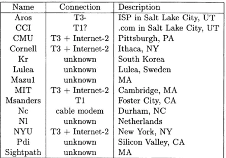
Figure 4-1: RON hosts and their characteristics

4.2

Chord Layer Tests

4.2.1 Evaluating the use of past latency data

Server selection at the Chord layer is mainly focused on finding the machine with the best latency. Each step of the lookup process takes little more than one round trip time for the closest-preceding-nodes request to be relayed to the server and the information for the next node on the lookup path to be relayed back. Ping times are thus closely correlated to the performance of the lookups. At the same time, since the time for a given step in the lookup path is roughly equivalent to the ping time between the two nodes, pinging

all the machines first to choose the fastest one adds a significant overhead to the overall performance. Instead, the selection mechanism must rely on past performance data to

choose a node.

In order to test whether past ping data is an accurate predictor of future performance, tests were run to determine how much latency between machines varies over time. If latency varies widely, past data would be a fairly useless metric unless it was taken very recently. If latency holds fairly steady, then the past ping times stored in each node would be sufficient to select the next server on the lookup path.

Name Connection Description

Aros T3- ISP in Salt Lake City, UT

CCI T1? .com in Salt Lake City, UT CMU T3 + Internet-2 Pittsburgh, PA

Cornell T3

+

Kr unknown South Korea

Lulea unknown Lulea, Sweden

Mazul unknown MA

MIT T3 + Internet-2 Cambridge, MA

Msanders Ti Foster City, CA

Nc cable modem Durham, NC

NI unknown Netherlands

NYU T3 + Internet-2 New York, NY

Pdi unknown Silicon Valley, CA

4.2.1.1 Methodology

The necessary data was collected using perl scripts running on every machine in the testbed. Every five minutes, the script would ping each machine in a list that included every other server in the testbed, plus an additional ten Web hosts, and record the ping results in a file. The Web hosts included a random assortment of more popular sites, such as yahoo, and less popular sites in both the US and Canada. They were included in the test to increase the data set, and to test the variance in latency for in-use, commonly accessed servers. These scripts were run several times for several days on end to get an idea of how ping times varied over the course of a day as well as over the course of different segments of the week. The resulting ping times between each pair of machines were then graphed over time, and the average, median, and standard deviation for the ping times were calculated. Since each ping only consisted of one packet, sometimes packets were lost between machines. Packet losses are graphed with a ping time of -1, but were not included in calculating the statistics. One point to note is that these experiments used ICMP ping, which may not be exactly representative of the actual behavior Chord will experience. Chord's lookup requests use a different communication protocol, which may therefore have different overheads and pro-cessing than the ICMP packets. Another experiment that may be interesting to conduct is to graph the round trip latencies for an actual request using the desired communication protocol.

4.2.1.2 Results

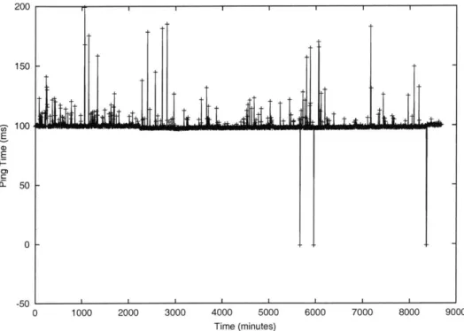
For the most part, results tended to look much like that in Figure 4-2. While individual ping packets sometimes experienced spikes in round trip time, overall the round trip latency remained steady over time. Some pairs of machines experienced greater variability in the size of the spikes, while others had far less variation. In general, machines with different performance tend to have fairly different ping times, and even with these variations, it is fairly obvious which are relatively better. Those that are closer in ping time tend to have more or less equivalent performance, so it does not matter as much if at a particular point in time, one has a better ping time than the other.

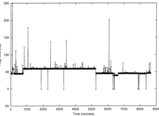
Several of the graphs depicted shifts in ping times such as those shown in Figure 4-3, and more drastically in Figure 4-4. Such shifts in latency are probably fairly common, and

200 150 100 E a) E 01 CL 50 0 -OU 0 1000 2000 3000 4000 5000 6000 7000 8000 9000 Time (minutes)

Figure 4-2: Sightpath to Msanders Ping Times

indicate rerouting somewhere in the Internet between the two machines. While it is evident that there will be a period of instability during which stored past latency data will not accurately predict future performance, for the most part, latency holds steady before and after the change. Therefore, while past latency data will not always be the best indicator, it is good enough the majority of the time.

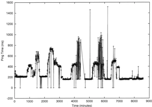
However, on occasion results look like Figure 4-5. Each of the large spikes in the graph seems to correspond to a different day of the week, indicating a great deal of variability during the daytime hours. The machines in question are connected to a cable modem in the US and at a university in Sweden. The higher spikes on weekends might indicate greater usage of cable modems when people go home on weekends; however, none of the other results to or from the cable modem show similar spikes. In fact, none of the other results to or from the Swedish machine show similar spikes either. The route between these two particular machines may be unusually congested and be more significantly impacted

by traffic over the Internet than the other routes. This graph is not very characteristic of

latency trends in this set of experiments, including the ping times to the web hosts that were not part of the testbed.

I IIt

-2 0I I I I I I I I 200 -150 -E 100 50 0 -50n

0

Figure 4-3: Cornell to Sightpath Ping Times

t

~ALLJ

~I1

1k d

TtX~

Lii

.1

It

t

It

Figure 4-4: Mazu to Nc Ping Times

9000 250 200

I

i4

17

It.

1600 1400 1200 1000 800 E M 600 400 200 0 -200 0 1000 2000 3000 4000 5000 6000 7000 8000 9000 Time (minutes)

Figure 4-5: nc to lulea Ping Times

4.2.2 Triangle Inequality

The Chord protocol has the option at each step of the lookup process to select from a pool of servers, some further in ID space than others, some closer in network distance than others. The proposed server selection method is to select a server closer in network distance (using round trip latency as the distance metric) at each hop, in the hopes of minimizing the overall latency of the lookup process. Due to the fact that the data used to determine network distance is actually an indirect measurement made by another node, this approach is based on the assumption that the triangle inequality holds true most, if not all, of the time. The ping times collected in the previous experiment were used to test this assumption.

There are actually three variations of the triangle inequality that were tested, each increasingly specific to this problem.

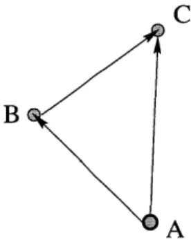
4.2.2.1 Simple Triangle Inequality

The first examined is what is normally meant by the triangle inequality, and is the only variation that actually involves a triangle. It states that if machine A is close to machine B, and machine B is close to machine C, then machine A is also close to machine C. This

C

B

<A

Figure 4-6: Simple Triangle Inequality

can be expressed as follows:

PingAB + PzTn9BC PingAC

This is generally useful since each step of the lookup algorithm essentially involves asking an intermediary node to find a third node.

In general, the triangle inequality is expected to hold. A direct path between two nodes should be shorter than an indirect path through a third node. However, network distances are a bit more complicated than physical distance. If the direct path is congested, lossy, or high latency, it may be ultimately slower than an indirect path made up of two fast links. This is somewhat akin to taking local roads to get around at traffic jam on a highway. Also, routers in the network may handle traffic in an unexpected manner, giving certain traffic higher priority than other traffic. Therefore, the triangle inequality should not hold all of the time.

4.2.2.2 Triangle Inequality Methodology

The simple triangle inequality was tested by collecting the ping data from the previous experiment in section 4.2.1, and finding all combinations of three machines where ping data existed between all three machines. Using this data, the components of the inequality were calculated, and the percentage of time the inequality held for all combinations of three machines was determined.

AB+BC=AC - -+ *+ + *+ + +I-+ +-H++ +++ ++ --+ + + +++U*+ + + -4 + ++ + + ++ + + + + ++++++ + + + + 0 200 400 600 800 AB + BC (ms) 1000 1200 1400

Figure 4-7: Triangle Inequality: AC vs AB+BC

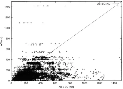
4.2.2.3 Triangle Inequality Results

All told, 20 different samples of ping times taken at different times over the five day period

were examined. Each of these samples consisted of a complete set of ping data taken from each machine at approximately the same time of day on the same day. Of the 30,660 combinations of 3 machines examined using these samples, the triangle inequality held for

90.4% of them.

Figure 4-7 pictorially illustrates how well these samples fit the triangle inequality. The diagonal line indicates the case when PingAB + PingBC = PingAc, and the triangle inequality holds for it and everything under it. This graph indicates that for the majority of cases, even those cases that do not fit the triangle inequality are not that far off. This is fairly consistent with the expected results and indicates that the triangle inequality can be assumed to hold in general.

1400 + +I4*-*-1200 -1000 -800 -600 -E 400 200 0

~1

X

B3

A

Figure 4-8: Relative Closeness

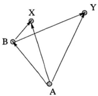
4.2.2.4 Relative Closeness

The second form of the triangle inequality is more restricted and specific. Instead of just determining if C is close to both A and B, this also tests relative closeness. Will asking an intermediate node for its closest machine also find the machine closest to the origin? In other words, if B says that it is closer to machine X than machine Y, will A also find that

it is closer to X than Y? This is determined by calculating if the following is true:

(PingAX < PingAY) == ((PingAB + PingBX) < (PingAB + PingBY))

This is equivalent to:

(Ping AX < PingAY) == (PingBX < Pin9BY)

This expression is more relevant to Chord lookups, since the proposed selection method uses indirect data to select close machines.

From a purely logical standpoint, assuming latency is directly correlated to geographic distance, if A, B, X, and Y are randomly chosen out of a set of geographically dispersed servers, there should not be any real correlation in relative closeness between A and B. A has just as good a chance of being close to X as it is to Y, and B, quite independently, also has an equal chance of being close to one or the other. Therefore, the relative closeness expression above should be true about 50% of the time.

4.2.2.5 Relative Closeness Methodology

For this test, a list of all machines to which there was ping data was compiled, including all 15 machines in the testbed and the 10 additional Internet hosts. These machines were used to generate all possible combinations of X and Y. Then, a different list of machines for which ping data from those machines was available was also compiled and used to generate all possible combinations of A and B. Using this data, the percentage of trials for which the above expression held was calculated for all combinations of A, B, X, and Y.

4.2.2.6 Relative Closeness Results

In this case, some 783,840 combinations of A, B, X, and Y were generated using the same 20 samples of data from section 4.2.2.3. Relative closeness held for 67.2% of ABXY combi-nations. This correlation is better than expected, and suggests that indirect data from an intermediary node may be useful for determining relative proximity from the origin server. The question may be raised as to why the correlation is better than random, since A, B,

X, and Y were essentially randomly chosen. The 50% correlation discussed previously

as-sumes a network in which the servers are evenly dispersed, and where latency is directly correlated to geographical distance alone. In an actual network, this may not be the case. The network is not arranged homogenously, with each server behind identical links and at regular intervals from each other. Instead, some machines may be behind very high speed, high bandwidth links in a well-connected AS, while other machines may be attached to high latency links that are somewhat removed from the backbones and peering points. While geographic proximity does contribute to latency, it is not the only factor involved. There-fore, some servers may frequently be relatively faster, while others are relatively slower, regardless of where the client is located.

This can be seen within the particular testbed being used in these experiments. Three of the machines in the testbed are in countries outside of the US, one in Korea, one in the Netherlands, and one in Sweden. The latencies to these machines are significantly higher than to any other machine in the US. Therefore, if one of these machines was X, then A and B will always agree that Y is closer. The results are also biased, because four of the machines are connected to each other via the Internet-2 backbone, which has considerably higher bandwidth and lower latency than the regular Internet backbone. Most of these