Changes in atmospheric eddy length
with the seasonal cycle and global warming
by
Todd A. Mooring
Submitted to the Departments of Physics
and
Earth, Atmospheric and Planetary Sciences
MASSACHUSETTS INSTITUTE OF TECHNOLOGY
JUN 0 8 2011
LIBRARIES
in partial fulfillment of the requirements for the degrees of
Bachelor of Science in Physics
ARCHIVES
and
Bachelor of Science in Earth, Atmospheric and Planetary Sciences
at the
MASSACHUSETTS INSTITUTE OF TECHNOLOGY
June 2011
@Massachusetts
Institute of Technology 2011. All rights reserved.
Signature redacted
A uthor
...
f
... o...
Todd A. Mooring
Departments of Physics and
Earth, Atmospheric and Planetary Sciences
Certified by...
Accepted
Accepted
Signature redacted
May 10, 2011
Paul A. O'Gorman
Assistant Professor
Department ofarth, Atmospheric and Planetary Sciences
Signature redacted
Thesis
Supervisor
b y ...
...
.. ...
Nergis Mavalvala
Undergra 4eh
is Coordinator, Department of Physics
by ...
.Signature redacted...
Samuel Bowring
Chair, Undergraduate Education Committee
Department of Earth, Atmospheric and Planetary Sciences
I-Changes in atmospheric eddy length with the seasonal cycle
and global warming
by
Todd A. Mooring
Submitted to the Departments of Physics
and
Earth, Atmospheric and Planetary Sciences
on May 10, 2011, in partial fulfillment of the
requirements for the degrees of
Bachelor of Science in Physics
and
Bachelor of Science in Earth, Atmospheric and Planetary Sciences
Abstract
A recent article by Kidston et al. [8] demonstrates that the length of atmospheric
eddies increases in simulations of future global warming. This thesis expands on
Kidston et al.'s work with additional studies of eddy length in the NCEP2 reanalysis
(a model-data synthesis that reconstructs past atmospheric circulation) and general
circulation models (GCMs) from the Coupled Model Intercomparison Project phase 3.
Eddy lengths are compared to computed values of the Rossby radius and the Rhines
scale, which have been hypothesized to set the eddy length. The GCMs reproduce the
seasonal variation in the eddy lengths seen in the reanalysis. To explore the effect of
latent heating on the eddies, a modification to the static stability is used to calculate
an effective Rossby radius. The effective Rossby radius is an improvement over the
traditional dry Rossby radius in predicting the seasonal cycle of northern hemisphere
eddy length, if the height scale used for calculation of the Rossby radius is the depth
of the free troposphere. There is no improvement if the scale height is used instead of
the free troposphere depth. However, both Rossby radii and the Rhines scale fail to
explain the weaker seasonal cycle in southern hemisphere eddy length. In agreement
with Kidson et al., the GCMs robustly project an increase in eddy length as the
climate warms. The Rossby radii and Rhines scale are also generally projected to
increase. Although it is not possible to state with confidence what process ultimately
controls atmospheric eddy lengths, taken as a whole the results of this study increase
confidence in the projection of future increases in eddy length.
Thesis Supervisor: Paul A. O'Gorman
Title: Assistant Professor
Acknowledgments
Many people contributed to the successful development of this thesis. Most of all I would like to thank Prof. Paul A. O'Gorman. He has been an excellent supervisor, from the moment I first walked into his office to inquire about UROP opportunities. He has always been available to answer my questions. listen to my ideas, and provide guidance about where the project should go next. I ani proud to be the first person to complete a thesis under his supervision.
Thanks also to my mother, Mary Kay Quinlan, for proofreading the thesis and trying to help ine manage my time. I hope I can successfully cone up with a non-mathematical explanation for her of what this thesis is actually about.
Jane Connor read drafts of the thesis and made a key suggestion for organizing the introduction. Alessondra Springnann read drafts as well.
Last but certainly not least. I would like to acknowledge the MIT Undergraduate Research Opportunities Program's de Florez fund. which provided financial support during the sunner of 2010.
Dedication
In loving memory of
Paul E. Quinlan
(1918-2010)
Contents
1
Introduction
2 Eddy Scales
2.1 Eddy length . . . . 2.2 Rossby radius . . . . 2.3 Rhines scale . . . .3 Effective Static Stability
3.1 Brief derivation. . . . .
3.2 Seasonal cycle of asymmetry parameter A . .
3.3 Seasonal evele of static stability parameters 3.4 Effective Rossby radius . . . .
4 Results-Seasonal Cycle
4.1 Northern hemisphere . . . . 4.2 Southern hemisphere . . . . 4.3 Causes of northern hemisphere seasonal cycle . . . .
5 Results-Global Warming
5.1 M
ultim
odel m ean . . . .5.2
Individual G CM s . . . .
6 Conclusion
15 19 19 20 22 23 23 25 26 28 31 32 33 33 43 43 45 53. . . .
. . . .
. . . .
. . . .
List of Figures
3-1 Seasonal cycles of asymnetry parameter A . . . . 27
3-2 Seasonal cycles of dry and effective static stabilities . . . . 29
4-1 Northern hemisphere length scale seasonal cycles (1) . . . . 34
4-2 Northern hemisphere length scale seasonal cycles (2) . . . . 35
4-3 Southern hemisphere length scale seasonal cyclcs (1) . . . . 36
4-4 Southern hemisphere length scale seasonal cycles (2) . . . . 37
4-5 Components decomposition of Leff northern hemisphere seasonal cycle 40 4-6 Components decomposition of LR northern hemisphere seasonal cycle 41 5-1 Fractional changes in L. LR (WMO) and LO over the 21st century . . 46
5-2 Fractional changes in L and LRea (WMO) over the 21st century . . . 47
List of Tables
5.1 Fractional increases in eddy scales froin 1981-2000 to 2081-2100 . . . 5.2
Quality
of fit of (6L,/L,.6L/L)
points to lines 6L/L =6L/L
. . .44
Chapter 1
Introduction
Transient eddies are the central dynamical feature of the extratropical atmosphere. The eddies transport heat and moisture poleward and thus play a key role in the Earth's climate system
[91.
An extensive body of work attempts to develop physical theories that explain the size of the eddies, which affects key aspects of their behavior such as propagation velocities and locations of dissipation [8, 221.The eddies exist because the atmosphere is baroclinically unstable [21]. The archetypal models of baroclinic instability are those of Charney. Eady and Phillips [2, 3, 14]. The models demonstrate how certain types of perturbations to a zonally symmetric flow on an
f-
or 6-plane can result in growing waves in the flow. The models yield predictions of the characteristic length scales of these waves [13, 221. For all three, the characteristic length scale isNH
f
where LR is referred to as the Rossby radius, N is the buoyancy frequency of the zonally symmetric flow, H is a relevant height scale., and
f
an appropriate value of the Coriolis parameter. The LR of equation 1.1 is then identified with the scale ofatmospheric eddies (e.g.. [18]).
It has also been suggested that the eddy length is set by the fundamental physics of rotating stratified turbulence. Theory predicts that the energy of the turbulett
flow shouki cascade to larger spatial scales. If f varies in the rotating system, as it
does for a planet or a 8-plane, the inverse cascade can be stopped by the gradient in
f.
limiting the size of the eddies to(3"RAIS 1/2
(1.2)
L3 is referred to as the Rhines scale, VRMJS is the RMS velocity of the flow, and 10 is
an appropriate valuc of df/dy [16. 22, 23].
Substantial debate exists in the literature on what sets the length scale of atmo-spheric eddies. Using simulations with a dry idealized GCM, Schneider and Walker (2006)
[181
argue that the Rossby radius and the Rhines scale vary similarly as the pole-cquator temperature gradient, planetary rotation rate and radius, and a convec-tive lapse rate are adjusted. Both length scales yield reasonable predictions of the eddy length exhibited by the GCM, and Schneider and Walker further argue that there is not in fact an inverse energy cascade and so the eddy length is set by the Rossby radius. Merlis and Schneider (2009) [11] describe linear stability analyses of the zonal mean flows of many of the simulations presented in [18] and several related works, strengthening the connection between the growing waves of the baroclinic in-stability and observed atmospheric eddies by demonstrating that the Rossby radius also scales with the zonal length scale of the fastest-growing baroclinic waves.Other studies suggest that the Rhines scale is the constraint on eddy lengths. Frierson et al. (2006)
[6]
adjust the amount of water vapor in the atmosphere of a moist idealized GCM and find that the Rhines scale is the best explanation of the resulting eddy lengths. Barry et al. (2002) [1] vary the pole-equator temperature gradient, planetary rotation rate and radius, radiative heating rate. and surface tem-perature in a moist GCM and calculate the eddy length, Rossby radius, and Rhines scale for each simulation. In this manner their study is similar to that of Schneider and Walker. However, Barry et al. find the Rhines scale to correlate better with the eddy length. The cause of the disagreement is unclear, but may relate to the substantial differences in the definition of eddy length between the two studies.Furthermore. the idea that the Rossby radius as defined in equation 1.1 deter-mines the eddy length scale of the real atmosphere suffers from a significant theoret-ical weakness. The dynamics of the real extratroptheoret-ical atmosphere are significantly influenced by latent heat release
[17],
but the baroclinic instability models from which the Rossby radius derives ignore this phenomenon. Studies of moist baroclinic insta-bility (e.g..[4, 5, 24]) suggest the need for modifications to equation 1.1 to include the effects of latent heating. Frierson et al. attempted to do so by making an ad hoc adjustment to N., but ultimately concluded that the Rhines scale was superior to thismodified Rossby radius in accounting for the eddy lengths simulated by their GCM.
Any effect of latent heating on eddy lengths mniay depend oi global temperatures.
because of the rapid increase in saturation specific humidity with temperature [17]. Evidence that global warming will affect eddy lengths is provided by Kidston et al.
(2010) [8]. who analyze the output of 12 GCMs from the Coupled Model Intercompar-ison Project phase 3 [10. Kidston et al. find that under the A2 emissions scenario, in which CO2 levels reach approximately 820 ppm by 2100, eddy lengths increase in
both hemispheres of each GCM studied. They argue that this process is linked to an increase in N, and use the NCEP/NCAR reanalysis to show that such an expansion
of the eddies may already be occurring.
Recent work by O'Gorman (2011) [12] provides a path forward on the problem of modifying the Rossby radius to account for the effects of latent heating. O'Gorman derives a way to parameterize the latent heating effect with an adjustment to N, facilitating its addition to the calculation of the Rossby radius and other atmospheric
dynamical quantities in which N is relevant. O'Gorman assesses the adjustment to
N using simulations with a moist idealized GCM. Eddy lengths are found to increase with global temperatures, in agreement with Kidston, and the changes are predicted
successfully by changes in the Rossby radius if the Rossby radius is calculated with the adjusted N. If the standard N is used, changes in the Rossby radius overestimate changes in the eddy length.
This thesis extends the work of Kidston and O'Gorman by using Rossby radii with
changes in eddy length projected by six of the CMIP3 GCMs. Unlike the idealized GCMs used in most of the studies described above, the CMIP3 models have seasonal cycles. This permits calculations of the seasonal variation of the Rossby radii, Rhines
scale, and eddy length in the simulated 20th century climate. Comparisons are made to the seasonal variations found in the NCEP-DOE Reanalysis 2 [7].
Chapter 2 of the thesis presents precise definitions of the eddy length, Rossby radius, and Rhines scale and explains how they were calculated from the GCM output
and reanalysis. Chapter 3 reviews O'Gorman [12] to describe how the latent heating effect is taken into account via an effective static stability and presents details of
the calculation of the effective static stability and the seasonal variation of static
stability parameters. Chapters 4 and 5 present results on the variation of the eddy
length, Rossby radii. and Rhines scale with the seasons and with global warming. respectively. Finally, conclusions arc presented in chapter 6.
Chapter 2
Eddy Scales
The calculations presented in this thesis are based on the output of six coupled
atmosphere-ocean GCMs (CSIRO-Mk3.5, ECHAM5/MPI-OM, CM2 .0,
GFDL-CM12.1., INI-CM3.0, and MRI-CCM2.3.2) from the Coupled Model
Intercompari-son Project phase 3 [10] and the NCEP-DOE Reanalysis 2 [7]. Characteristic values of the eddy length L, the Rossby radius LR and the Rhines scale L3 were calculated
for the latitude bands of 30-70 degrees in each hemisphere.
In the following discussion of how the various eddy scales were computed, a clear
distinction must be drawn between zonal means and averages over latitude bands of finite width. The zonal and time mean of a quantity (-) will be denoted by (.). The
area-weighted time mean over latitudes
[@min,
emax] is then1 a-x
((0)) =
(-)
cos 0 do. (2.1)Sn 11 max Sil s 1i Omiem
2.1
Eddy length
A characteristic eddy length seale is defined using meridional winds at 300 hPa. To
capture the transient eddies, daily-mean winds were filtered using a 13th-order
high-pass Butterworth filter with a six-day cutoff to produce eddy meridional winds v'(O, V) where
#
is the latitude and x is the longitude. At each latitude, the v'(0, x) were Fourier transformed and squared to compute the energy in each zonal wavenum-ber and then time averaged to create a tifle-averaged eddy kinetic energy spectrum V2(0, k) where k is the zonal wavenumber.
At every latitude each zonal wavenumber can be associated with a local zonal wavelength
27ra cos
(
f #
)
k
(2.2)
k
where a is the radius of the Earth. An eddy length is then computed over the full latitude band of integration by taking an energy- and area-weighted mean of the local zonal wavelengths
L
=kZz-r(O,
k)V
2(6,k))
(2.3)(Zk
"' V2(0,k))
2.2
Rossby radius
As discussed in the introduction, the Rossby radius is a characteristic length scale that emerges from the imodcls of baroclinic instability of Charney, Eady, and Phillips [2, 3.
13, 14, 22]. It is convenient to express the terms on the right hand side of equation 1.1
in pressure coordinates, and similarly to Merlis and Schneider
[11]
and O'Gorman [12] the Rossby radius LR will be definedLR=
2 NPAp)
(2.4)f
where NP is a static stability parameter
1 51/2
NP-
_
,
(2.5)
Ap is a relevant height scale in units of pressure, and
f
is an appropriate value of the Coriolis parameter.0
is the potential temperature and p is the density of the air. respectively.As in Kidston et al. [8] and O'Gorman
[121,
NP is evaluated in the lowertro-posphere (850-600 hPa) using zonal- and time-mean temperature and geopotential height fields.
00/ap
was calculated using a finite difference between 850 and 600hPa, while p and
0
are density-weighted vertical means. Aside from the convenience of consistency with previous studies, the 850-600 hPa region is a reasonable choice of evaluation level because it is a region where the growing baroclinic waves char-acterized by the Rossby radius have relatively large amplitudes[11].
There is some uncertainty about how to evaluate Ap. The Eady model of baroclinic instability fea-tures fixed walls at the top and bottom. and the upper wall can be identified with the tropopause [22]. Ap is then the free troposphere depth. The tropopause is diagnosed from temperature and relative humidity data using the WMO tropopause definition as the lowest level at which the lapse rate drops to 2 K kim 1 and an algorithm similar to that given in[151.
(For computational simplicity, the WMO definition that the mean lapse rate between a putative tropopause and any point within 2 km above it not exceed 2 K kin 1 has been slightly altered to require that the lapse rate at every level within 2 km above a putative tropopause be less than 2 K kin'.) The free troposphere is assumed to begin at 850 hPa instead of the surface, to exclude the planetary boundary layer, and Ap is calculated as the difference between 850 hPa and the tropopause pressure. The issue of the vertical scale in the Charney model is more complex, but in one limiting case the vertical scale is the scale height[131.
In this case. it (;an be shown that Ap is equal to the mean value of the pressure in the levels being used to determine NP. For the Phillips model, the height scale is the depth of the fluid, which can again be identified with the free troposphere depth [22].The latitude for the evaluation of
f
was determined by identifying the maximum in the time-mean eddy meridional temperature transportXITTe
ddy=27rav'(O, X)T'(0.
x)
cos e, (2.6)where T'(0, X) is the eddy temperature calculated by filtering daily-mean tempera-ture fields with the same Butterworth filter used to determine v'(6, x). To evaluate equation 2.6, u'(#. x) and T'(0, x) were computed at 850 hPa. Some calculations were
also
done
withf
evaluated at a latitude QMTT givenby
(#
&(#,
)T'(#,
x))
(27
MVTT
(2.7)
(6(1
X)T'((), X))
where again
c'(6,
x)
andT'(b,
x)
were evaluated at 850 hPa.To evaluate equation 2.4, an area-weighted mean value of the numerator (NPAp) is computed over the 30-70 degree integration region and then divided by f evaluated at the latitude with the maximum value of MTTddy or at OMTT.
2.3
Rhines scale
The Rhines scale [16. 22, 23] is defined by
L = V , /2 4 (2.8)
Q 3)l/2
where (v'2) is a time and spatial mean over the region in question of the eddy kinetic energy
,'
2(,
x)
at 300 hPa and3
is evaluated at some appropriate latitude.3
is evaluated at the latitude of the maximnum inEKE
V'2 (, x) cos . (2.9)Chapter 3
Effective Static Stability
0'Gorman's addition [12] of the effects of latent heat release to large-scale
dry-atmosphere dynamical theories, such as baroclinic instability problems, is
accom-plished by replacing the traditional dry static stability where it appears in such
the-ories with an appropriately-defined effective static stability. This chapter reviews
the derivation of the effective static stability and analyzes the seasonal cycle of an
asymmetry parameter A that is invoked in the derivation. It then discusses the
sea-sonal cycles of the dry static stability parameter NP and its moist counterpart Neff
and concludes by formally presenting the definition of an eddy scale LReff, a Rossby
radius evaluated using the effective static stability.
3.1
Brief derivation
The full derivation of the effective static stability is given in [12] and will not be
reiterated here. In summary, it involves consideration of the changes in dry potential
temperature 0 and equivalent potential temperature 0* of a saturated air parcel. If
diabatic heating and cooling are ignored, 0* will be conserved following the parcel's
motion and thus
DO
HO
=
_-(3.1)
where H(.) denotes the Heaviside step function,
w
= Dp/Dt is the vertical pressurevelocity, wt = H(-w)w, and the 0* subscript on the partial derivative indicates that
the partial derivative is taken at constant
0*.The Heaviside step function appears
because condensation and latent heat release are being approximated as occurring
always and only when the parcel ascends.
For purposes of this derivation, eddy quantities will be defined as departures from
the zonal mean and denoted (.)'. Denoting a zonal mean at fixed time by
(.),
it can
thus be shown that
00'
- 3 i8=
-
'-
+ W
-*
,
(3.2)
at (9p OP
if the partial derivatives of
0'with respect to pressure are set to zero. It is easy to
see that the first term of this equation is associated with the advection of dry air
through the point at which the equation is evaluated, while the second term comes
from latent heat release in rising air. In a dry atmosphere, this second term would
disappear.
The effective disappearance of the second term of equation 3.2 in the real moist
atmosphere can be achieved by folding it into the first term. This is accomplished by
writing
=
Aw' +
C,
(3.3)
where A is a constant that is regressed for using w' and w ' taken from GCM output
or reanalysis. Then, taking wT' ~ Aw', equation 3.2 can be rewritten
00 -
[
=
+
A
-
.(3.4)
t
ap
ap
The quantity in brackets in equation 3.4 is defined as the effective static stability
--
=--
+A
-
.
(3.5)
eff O 0*
A is related to the up-down asymmetry of the eddy vertical velocity field, so it will
When equation 3.5 is substituted into equation 3.4. equation 3.4 acquires the same
functional form as the dr-atnosphere version of equation 3.2. Thus the effects of latent heating can be parameterized by substituting --
O/&pleff
for -0/8p wherever the latter appears. Because saturated air moving upwards is warmed by latent heatrelease, 0O/&plo. < 0 and so the effect of latent heating is to reduce the effective static stability of the atmosphere relative to the dry value.
3.2
Seasonal cycle of asymmetry parameter A
The value of the effective static stability as a conceptual tool for analyzing moist atmospheric circulations is partially dependent on A remaining relatively constant with the seasonal cycle and with global climate change. Although O'Gorman
[12]
notes that some previous works on moist baroclinic instability([4,
5., 241) imply A -+ 1 with the increasing specific humidity that would occur with global warming, idealizedGCM simulations presented in that study nevertheless suggest a A largely independent
of temperatures.
Using the output of the idealized GCM, O'Gorman [12] calculated average values
of A over the full areal and vertical extent of the extratropical troposphere. They changed by just 0.02 (from 0.59 to 0.61) as the GCM's global mean surface temper-ature was increased from 270 to 316 K. However, the idealized GCM has simplified parameterizations, a global mixed layer ocean as the lower boundary, and no seasonal or diurnal cycles. The constancy of A in more realistic models of the climate system
and the real world as represented in NCEP2 is thus worth investigating.
Evaluation of A requires w data at high temporal resolution. The monthly-mean
values archived in the CMIP3 dataset are inadequate for this purpose, so A was evaluated only for NCEP2, using 4x daily w data for 1981-2000. It can be shown that at a single time, latitude, and pressure level
and for simplicity the time-mean A is evaluated using the approximate equation
A ww 7 1
(37)
After computing A as a function of latitude and pressure for each month, monthly regional nean values
(A)
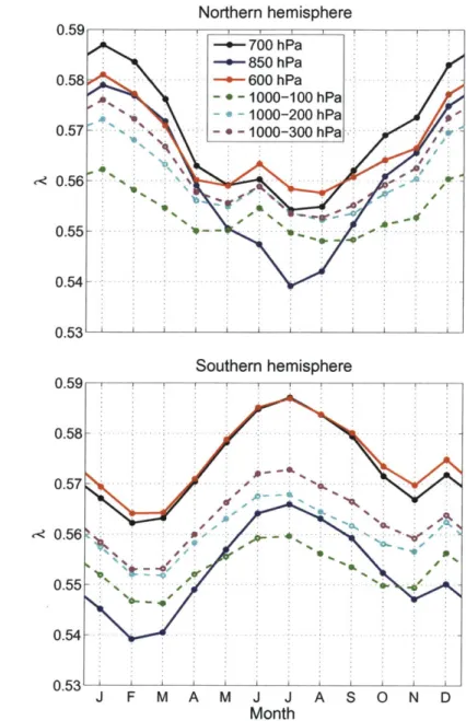
over 30-70 degrees in each hemisphere were calculated usingA values at 850, 700, and 600 hPa. Several additional calculations also took
mass-weighted depth averages of A over 1000-300, 1000-200, and 1000-100 hPa, for more direct comparability to the idealized GCM results. The resulting seasonal cycles of A are presented in Fig. 3-1. Although the amplitudes of the seasonal cycles in these hemisphericallv-averaged A values are comparable to the change in the idealized GCM's annual mean A over a very large range of global temperatures. it can be shown that these variations are still small enough to approximate A in all seasons and both regions by the average of the two regional annual mean values of A at 700 hPa. It is interesting to note that A values peak during the winter and are minimized during the sunner. This is the opposite of what would occur if the regionally-averaged A values were increasing functions of regional-mean temperatures. as one might expect based on the temperature dependence of A documented in [121.
3.3
Seasonal cycle of static stability parameters
Because A is apparently adequately stable over the seasonal cycle and with a changing climate, the effective static stability can be readily used to parameterize the effect of latent heating on atmospheric eddies. As a complement to the traditional dry static stability parameter NP defined in equation 2.5, it is possible to define an effective static stability parameter
(1
& I/2 (1Fa9
_i
N
= - - --
A
/(3.8)
where the zonal means at fixed time in equation 3.5 have been replaced by zonal and time means.
0.59 0.58 0.57 0.55 0.54 0.53 0.58 0.57 e
0.56
0.55 0.54 0.53 Northern hemisphere 700 hPa -+-850 hPa 600 hPa - - 1000-100 hPa -1000-200 hPa .- -1000-300 hPa Southern hemisphere J F M A M J J A S O N D MonthFigure 3-1: The seasonal cycles of A computed using 30-70 degrees in each hemisphere
and various levels of the atmosphere. The underlying 4x daily
w
data was taken from
the 1981-2000 subset of the NCEP2 reanalysis. Clear seasonal cycles are present
for all methods of A evaluation, although depth averaging tends to reduce the cycle
amplitude. Values of A were not available at 1000 hPa for every latitude. Although
the depth averages list 1000 hPa as the bottom of the integration region for both
hemispheres, the integration extended only as far down as 925 hPa in the northern
hemisphere. In the southern hemisphere, 1000 hPa A values were available for 30-50
degrees S in most months. At 70 degrees S, A was unavailable at 925 hPa and the
vertical integration was stopped at 850 hPa.
To investigate the importance of the latent heating effect, (NP) and (N'ff) were computed for each calendar month and GCM/reanalysis using data from latitudes
30-70 degrees in each hemisphere and years 1981-2000. Rather than analyzing each of
the six CMIP3 GCMs individually, the monthly values for each GCM were averaged to form multimodel monthly means. The NCEP2 reanalysis was not included in the means and was studied separately.
The seasonal cycles of (NP) and (N'ff) are plotted in Fig. 3-2. The multimodel mean and NCEP2 seasonal cycles are similar in nearly every respect. In both hemi-spheres, the effective static stability parameter is clearly smaller than its dry counter-part. In the northern hemisphere, the inclusion of the latent heating effect substan-tially increases the amplitude of the seasonal cycle in both absolute and fractional senses and alters its phase. In contrast, the absolute amplitude of the southern hemi-sphere seasonal cycle is reduced. The substantial differences between (NP) and (N'ff) suggest a significant influence of latent heat release on the behavior of the midlatitude atmosphere.
3.4
Effective Rossby radius
NPf can be used to calculate an effective Rossby radius, defined in analogy to
equa-tion 2.4 as
LReff = 27 (NffAp (3.9)
f
As in the definition of the dry Rossby radius (equation 2.4), p, 0, and the pressure derivatives of potential temperature in equation 3.8 were evaluated using data from
850-600 hPa. A was evaluated at 700 hPa. The latitude of
f
evaluation was found using the same methods as for LR. Equation 3.9 was evaluated by finding (Nff Ap) over 30-70 degrees in the hemisphere of interest, the same integration region used for the eddy scales described in chapter 2.Multimodel mean - - ---1.6 U) 0.E 1.4 C) 1.2 CU CU CO, Ca C)0.8 NCEP2 Cu CU 1.4 o .2 CU CU, U) 0.8 J F M A M J J A S O N D -- (N ) (NH) (NeF) (NH) - (N) (SH)
Figure 3-2: (NP) and (N') are displayed for both hemispheres in each panel. Solid
lines indicate quantities evaluated using 30-70 degrees N, while dashed lines indicate
quantities evaluated using 30-70 degrees S. In both hemispheres the effective static
stability is reduced substantially relative to the dry static stability. (NP) and (NP )
were calculated using temperature and geopotential height fields from 850-600 hPa,
Chapter 4
Results-Seasonal Cycle
The studies reviewed in chapter 1 analyze eddy scales in idealized GCMs in which parameters are varied, or changes in annual mean eddy lengths in more realistic GCMs and reanalysis. None of the idealized GCMs included a seasonal cycle. Accordingly. analysis of the seasonal variability of the eddy scales described in chapters 2 and 3 may provide additional information about the physical causes of observed and modeled
eddy lengths. The northern and southern hemispheres will be discussed separately.
because of substantial qualitative differences in both the character of the eddy length seasonal cycles and the success of the various Rossby radii and the Rhines scale in predicting the cycles.
As in chapter 3, a mean value of each eddy scale was determined for each calendar month and GCM/reanalysis using data from 1981-2000. The monthly values for each
GCM were averaged into multimodel monthly means, while the NCEP2 results were
kept separate.
The LR. LReff. and L3 described in chapters 2 and 3 can be thought of as predic-tions of the eddy length L. However, the underlying theories predict the existence of unstable waves of a range of wavelengths and so cannot be interpreted as yielding particular exact values for L. Accordingly., the Rossby radii and Rhines scale sea-sonal cycles were all rescaled for the best fit to the L seasea-sonal cycle before making any comparisons.
theoretical characteristic length scale L,. where Lx is one of the Rossbv radii or the Rhines scale, were related by a rescaling constant c such that L = cL. It can be
shown that the least-squares best-fit value of c is given by
C = L . (4.1)
where i indexes over months. c was evaluated separately for each Lx and hemisphere.
4.1
Northern hemisphere
The seasonal cycles of eddy length, various Rossby radii, and the Rhines scale for the northern hemisphere are displayed in Figs. 4-1 and 4-2. The Rossby radii and Rhines scale have been rescaled for the best fit to the eddy length seasonal cycle as described above. The multimodel mean of the GCM eddy lengths exhibits a distinct seasonal cycle, with the eddies at their longest in the northern hemisphere
winter. The multimodel mean eddy length seasonal cycle compares favorably with the eddy length seasonal cycle in the NCEP2 reanalysis, and indeed the qualitative
relationships among all seasonal cycles plotted are basically the same for both the multimodel mean and NCEP2. This suggests a remarkable degree of success by the
GCMs in reproducing observed seasonal variations in atmospheric eddy activity.
In Fig. 4-1, the seasonal cycles of both Lueff and L,3 are qualitatively quite similar
to the L seasonal cycle. The amplitude of the LReff cycles is somewhat too large,
although this overestimate is reduced by the use of OMTT instead of the latitude of the maxinmum in MTTeddy for the evaluation of
f.
In contrast, the amplitude of the L8 seasonal cycle is too small. L, is also notably too constant in January-April.Agreement of the LR seasonal cycles with the L seasonal cycle is less impressive,
particularly if the 1MTT method of selecting the
f
evaluation latitude is used.Fig. 4-2 displays a number of the same seasonal cycles as Fig. 4-1 but shows
seasonal cycles of LR and LRef with Ap identified as the scale height of the atmosphere instead of the free troposphere depth. Pursuant to the discussion in section 2.2, Ap
is taken as 725 hPa. However, this choice does not actually matter because since Ap does not change with the seasons, it is essentially an arbitrary constant factor whose effects will be eliminated by the rescaling that is applied before plotting.
The principal conclusion to be drawn from Fig. 4-2 is that the use of the scale height in place of the free troposphere depth as the value of Ap in Rossby radius calculations increases the amplitude of the resealed seasonal cycle. In contrast to the results displayed in Fig. 4-1, this choice results in LR being a comparable or better fit to the eddy length seasonal cycle than LReff.
4.2
Southern hemisphere
Figs. 4-3 and 4-4 display eddy length, Rossby radii, and Rhines scale seasonal cycles for the southern hemisphere. Both the multimodel mean and NCEP2 seasonal cycles are again similar, although the cycles themselves are strikingly different from their northern hemisphere counterparts. The annual mean eddy length is noticeably larger, and its seasonal cycle amplitude is smaller. Additionally, the eddy length seasonal cycle is no longer generally sinusoidal in shape.
Unlike in the northern hemisphere, none of the Rossby radii or Rhines scale sea-sonal cycles appear to succeed in explaining the eddy length seasea-sonal cycle. Although the resealed Rossby radius and Rhines scale cycles have reasonable amplitudes, they are not able to reproduce the January-February minima and September-October max-ima that characterize the eddy length seasonal cycle. The choice of the free tropo-sphere depth or the scale height for Ap makes little difference to the Rossby radii seasonal cycles.
4.3
Causes of northern hemisphere seasonal cycle
To study the causes of the seasonal cycle in eddy length, the seasonal cycles of the dry and effective Rossby radii plotted in Figs. 4-1 and 4-2 were decomposed into their components. Only results from the northern hemisphere are presented, as the failure
Multimodel Mean NCEP2 -. ....-. - ...-. ...---..- ..---... -- - -zOUU J F M A M J J A S 0 N D Month
Figure 4-1: Seasonal cycles of eddy length, various dry and effective Rossby radii,
and the Rhines scale over 30-70 degrees N during 1981-2000. The Rossby radii
la-beled (max) had
f
evaluated at the latitude of the maximum in
MTTeddydefined
in equation 2.6. Rossby radii labeled (mean) had f evaluated at
4MTT
as defined in
equation 2.7.
MTTddyand
OMTTwere evaluated at 850 hPa, and the free troposphere
depth was used as Ap. For the Rhines scale, 0 was evaluated at the latitude of the
maximum in EKE (equation 2.9).
34 0 L Reff -0 Lef (mean) 0 LR (mx - -L (mean) 0 450 400 O 350 Cm C: 0) -J 300 250 4500 4000 E O 3500 U 30 3000
'
Multimodel Mean 4500 4000 3500 3000 2500 4500 4000 a) L 3500 CD ca a) -j ' J F M A M J J A S O N D Month
Figure 4-2: Seasonal cycles of eddy length and various dry and effective Rossby radii
over 30-70 degrees N during 1981-2000. The Rossby radii labeled (WMO) had the
height scale /p in equation 2.4 or 3.9 defined as the free troposphere depth. Rossby
radii labeled (H) had Ap identified as the scale height. In all cases
f
was calculated
at the latitude of the maximum in MTTddy, evaluated at 850 hPa.
LReff (WMO) - * -Re(H)-. (WMO) -o-LR(H) NCEP2 3000 I ... ... - -
-4500 4000 3500 U, ) -J 3000 2500 4500 4000 3500 a) -j 3000 Multimodel Mean ..- - .. . . . . ... .. ... . .
~*
- - -(ean - -L -L (max) - -LR (mean) L NCEP2 4 9 ... .. . . . -...-..-..-.. . -.. ..........-..--.. ..... ...... J F M A M J J A S 0 N D MonthFigure 4-3: Seasonal cycles of eddy length, various dry and effective Rossby radii,
and the Rhines scale over 30-70 degrees S during 1981-2000. The Rossby radii labeled
(max) had
f
evaluated at the latitude of the maximum in MTTeddy. Rossby radii
labeled (mean) had
f
evaluated at
$MTT.Both
MTTddyand
OMTTwere calculated
at 850 hPa, and the free troposphere depth was used as Ap. For the Rhines scale,
#
was evaluated at the latitude of the maximum in EKE.
36
Multimodel Mean 4500 4000 -... E CO 03500 -CO, - -- (WMO)
3000
- _ LRf (H) - LR(WMO) -0-L (H) 2500 NCEP2 4500 03500Q 3000 2500 . J F M A M J J A S O N D MonthFigure 4-4: Seasonal cycles of eddy length and various dry and effective Rossby radii over 30-70 degrees S during 1981-2000. The Rossby radii labeled (WMO) had the height scale Ap defined as the free troposphere depth, while Rossby radii labeled (H) had Ap identified as the scale height. For all cases f was calculated at the latitude of the maximum in MTTddy. MTTddy was evaluated at 850 hPa.
of any Rossby radius seasonal cycle to predict the eddy length seasonal cycle in the
southern hemisphere suggests that little is to be learned about the seasonal variation
of southern hemisphere eddies by studying corresponding Rossby radii.
Referring to equation 2.4, the dry Rossby radius in any given month i is denoted
by
LRi= 2
7(NPAp), =
2(NP)(Ap)i + (NPa(O)Ap(#))j
(4.2)
fi fi
where the departure of a quantity
(-)
from its regional mean value
((.))
is denoted by
().
Because
NP,
Ap, and
f
are all in different units of measure, the monthly variations
of these quantities must be written in a nondimensional form to meaningfully compare
the contributions of changes in each to the changes in
LR.If for a quantity
(-)
a
monthly anomaly for month
iis defined
6(-)i
=H-)- (-),
(4.3)
where
()
denotes the annual mean of
(-),
equation 4.2 can be rewritten
LRi
= 21 j[(NP)+ 6(NP)][(Ap) +
5(Ap)]
f [1 +
6ft/f]
where it has been assumed that
(NPa(#)Apa(O)),<<
(NP)j(Ap)jand so the second
term in the numerator of equation 4.2 can be dropped.
1
By additionally assuming that (I +
6fi/f)
1-6fi/f, expanding equation 4.4,
and dropping all terms with more than one 6(-), it can be shown that
3LRi 6(NP)i 6(Ap)_
6fi
-7: = + - - (4.5)
LR (NP)
(.p)5
in which all quantities appear in the desired nondimensional form. Equation 4.5 is of
course valid for effective Rossby radii as well, when
LRis replaced by
LReffand
NP
by NPff.
Figs. 4-5 and 4-6 show both sides of equation 4.5 along with each individual
term on the right side of the equation for both dry and effective Rossby radii. The good match between the normalized Rossby radii seasonal cycles and the sum of the seasonal cycles of the components suggests that the approximations made in deriving equation 4.5 are good ones. In view of the results displayed in Figs. 4-1 and 4-2, it is not surprising that very similar results are obtained for both the multimodel mean and NCEP2.
As was previously shown in chapter 3, the effective static stability parameter
(Neff)i exhibits a clear seasonal cycle with the maximum in January and the minimum
in July. In contrast, the dry static stability parameter (NP)i has a fractionally much smaller seasonal cycle with maxima in November or December and minima in May or June. The troposphere depth is maximized in August and minimized in February, while the latitude of the maximum in MTTddy reaches its northern extreme in August and is farthest south in February or March.
The troposphere depth and f evaluation latitude seasonal cycles are of similar amplitude and phased so as to have a tendency to cancel each other out. Because
(Ap)i is time-independent when Ap is identified as the scale height of the
atmo-sphere, 6(Ap)i/(Ap) = 0 and the cancellation effect disappears. Since -6fi/f) varies roughly in phase with
(Neff)j
and is considerably larger than the(NP)j
seasonal cycle, the fractional amplitude of rescaled Rossby radius seasonal cycles with Ap identified as the scale height is larger than when Ap is identified as the free troposphere depth. This is consistent with Fig. 4-2.Finally, it appears that the relatively noisier character of the NCEP2 seasonal cycles as compared to their multimodel mean counterparts, clearly visible in Figs. 4-1 and 4-2, derives mainly from noise in the seasonal cycle of the
f
evaluation latitude. The relative suppression of this noise in the multimodel mean likely results from the average taken over six GCMs.Multimodel mean 0.2 -0.35 - -- Nf1(~f+H/H-f/ 0 .1 -... -. ...-. -. -.-0.05 0- --0.05 . -. -.. -. ... . -0.1 -0.15 --0.2 ... ... ... ... ... ... -0.25 __S~fiRf -0.3 * _SNP /(NP)+8H./(H)-8f,/f NCEP2 S)F MA /JJ 0.2 _ 8 H /(H) 0 .1 5 -. .. ...-. ..-.. ..- ... -..._..._. -5f /f 0 .1 . . ... ... . ... .... ..-. -.
Figur 4-5:
...
Normlize seasonal
cycles... of....
L.ff.is.omonns.ccrdngtoeqa
0.05---0
-40
-0 .1 - .... -... -.. ... ... . ... .... ...-.. -0 .1 5 - ... ... - .. .. .-.. -.. -.--0.2 - ..-..- -0.25--0.3 J F M A M J J A S 0 N DFigure 4-5: Normalized seasonal cycles of LRef, its components according to equa-tion 4.5, and their sum.
f
was evaluated at the latitude of the maximum in MTTddl,. Note that the curve associated with the variations off
is actually -Jfi/f (the August minimum in -6fi/f is when the latitude of evaluation off
is at its northern extreme and f is maximized). MTTeddy was evaluated at 850 hPa. Hats have been dropped from the text in the legend.Multimodel mean 0.2 0.15 - -.-.-0.1 0.05 -0 -0.25 . . * . .. -.. -0.25 - -.._...L.) -0.3 I I - - NP/(NP)+SH./(H)-8f./f NCEP2
SP(P
-0.1 -0 .1 ...- ... -.. .... ... ...-. -.. -0.25 --0.3 J F M A M J JAS ON
DFigure 4-6: Normalized seasonal cycles of
LR,its components, and their sum. Note
the greatly reduced amplitude of the NP seasonal cycle relative to the N'ff cycle in
Fig. 4-5.
f
was calculated at the latitude of the maximum in
MTTeddyand
MTTeddywas evaluated at 850 hPa.
Chapter 5
Results-Global Warming
According to Kidston et al. [8], CMIP3 GCMs robustly project an increase in
atnio-spheric eddy lengths over the 21st century. To confirm and further understand this result. annual mean values of the various eddy scales were computed for each of the six GCMs for 1981-2000 and 2081-2100. The GCMs were run for a number of possible emissions scenarios for the 21st century. Only the moderate AlB scenario, in which CO2 concentrations reach approximately 550 ppm by 2100, is considered here [10]. The annual means were used to compute fractional increases
6L L1 - L20
___ X
(5.1)
LX L20
where L20 and L21 denote 1981-2000 and 2081-2100 annual mean eddy scales and 6(.) now represents the difference between 2081-2100 and 1981-2000 annual means of a quantity (.). instead of a monthly anomaly.
5.1
Multimodel mean
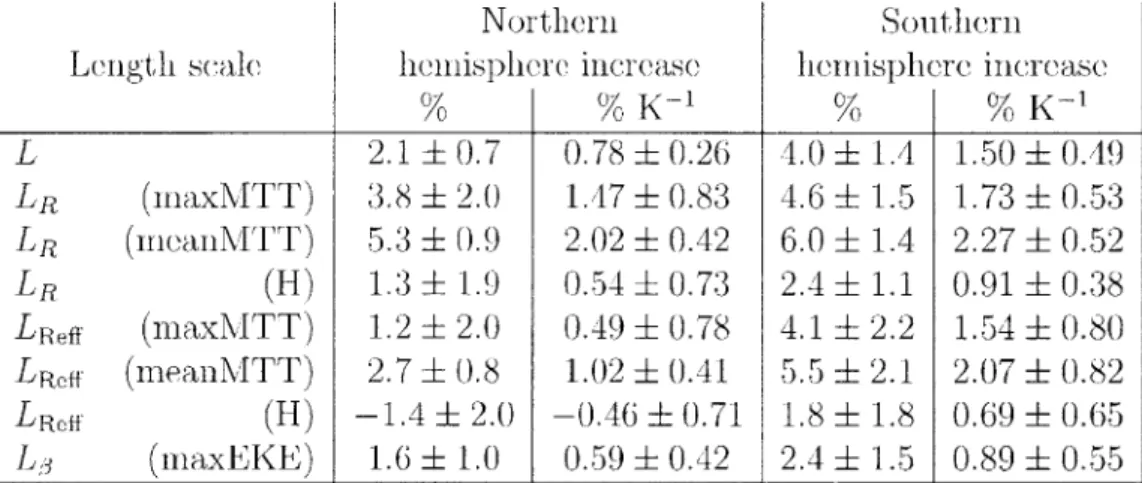
The multimodel mean increases and multimodel mean increases per K of rise in the global mean surface temperature are listed in Table 5.1, along with the multimodel standard deviation to characterize the scatter among the different GCMs. The mul-timodel mean values of all but one of the eddy scales computed are found to increase
Table 5.1: Multimodel mean fractional increases and fractional increases per K of global mean surface temperature increase are listed for various eddy scales. The increases are calculated using the differences between the 2081-2100 and 1981-2000 means of each eddy scale. For the eddy scale increase per K of temperature increase, the temperature increase is calculated as the difference between the 2081-2100 and
1981-2000 means. The intermodel scatter (one standard deviation) is also given for
each quantity. In the first column, (maxMTT) denotes evaluation of
f
at the lati-tude of the maximum in AMTTddy and use of the free troposphere depth to defineAp. (meanMTT) indicates evaluation of
f
at the latitude OJd T, again with the free troposphere depth used to define Ap. Eddy scales marked (H) hadf
evaluated at the maximum of AITTeddy but used the scale height as Ap. (maxEKE) indicates evaluation of 0 at the latitude of the maximum in EKE. MTTddy and OMTT were evaluated at 850 hPa, while EKE was evaluated using winds at 300 hPa.Northern hemisphere increase
%
% K-
1 Southern hemisphere increase %-% K-1
L 2.1 0.7 0.78 0.26 4.0 1.4 1.50 0.49 LR (maxMTT) 3.8 2.0 1.47 0.83 4.6 1.5 1.73 0.53 LR (meanMTT) 5.3 0.9 2.02 0.42 6.0 1.4 2.27 0.52 LR (H) 1.3 1.9 0.54 t 0.73 2.4 1.1 0.91 0.38 L Ref (maxMTT) 1.2 2.0 0.49 0.78 4.1 2.2 1.54 0.80 LReff (meanITT) 2.7 0.8 1.02 0.41 5.5 2.1 2.07 0.82 LReff (H) -1.4 2.0 -0.46 0.71 1.8 1.8 0.69 0.65 L3 (maxEKE) 1.6 1.0 0.59 0.42 2.4 1.5 0.89 0.55between 1981-2000 and 2081-2100. However, in a number of cases the positive value of the increase is within one standard deviation of zero. (The sole decline is also
within one standard deviation of zero.)
The multimodel mean eddy scale increases per K of temperature increase are also positive in all but one case, and generally at least one standard deviation above zero.
In addition, the multimodel mean of every eddy scale exhibits a larger fractional
in-crease (or smaller fractional dein-crease) in the southern hemisphere than in the northern hemisphere. But for some individual models and eddy scales, fractional increases are
larger in the northern hemisphere. Length scale
5.2
Individual GCMs
To further investigate the modeled increases in eddy scales, fractional increases in
L are plotted against fractional increases in the various LR, LReff, and L'3 for each
GCM and hemisphere in Figs. 5-1, 5-2, and 5-3. The eddy length and Rhines scale
are found to increase for all models and hemispheres, as do the dry Rossby radii for all but one combination of model, hemisphere, and
f
evaluation latitude/Ap. The effective Rossby radii results are more complex, with the choice of the scale height rather than the free troposphere depth for Ap clearly reducing values of 6LReff/LReff-For four of the six GCMs, northern hemisphere values of LReff calculated with the scale height as Ap are in fact projected to decline over the 21st century.
Although the changes are positive for most models, hemispheres, and eddy scales, they nevertheless vary considerably among GCMs. Using a method similar to that in
[8], if it is assumed that the fractional increase in eddy length 6L/L for each model is
perfectly explained by the fractional increase in one of the other eddy scales 6LX/L, the points (6Lx/LX, 6L/L) for all six GCMs should fall on the line 6L/L = 6L/L.
Accordingly, analysis of the intermodel scatter in values of the fractional increases in the eddy length, the Rossby radii, and the Rhines scale could yield insight into the causes of the modeled eddy length increase.
Inspection of Figs. 5-1, 5-2, and 5-3 indicates that the simple ideal of a clear
6L/L = 6Lx/L, for a single Lx does not describe the behavior of the GCMs. For all of the Lx studied, the southern hemisphere values of 6L/L do generally increase with increasing 6Lx/Lx. However,
6L/L
can be systematically underestimated (asby 6LReff/LReff with
f
at the maximum in MTTddy and the scale height as Ap) or overestimated (as by 6LR/LR with f evaluated at OMTT and the free troposphere depth as Ap). This roughly monotonic relationship between 6L/L and 6Lx/Lx does not carry over to the northern hemisphere. Instead, (8Lx/Lx,6L/L) points form clumps or spread out over larger ranges in 3Lx/Lxthan in 6L/L.
hypothe-0 .hypothe-0 8 - ...-.. -... ... ... 0.06
V
"0 0 .0 4 -.. ... ... .. 0.020
0
0.02 0.04 0.06 0.08 0 0.02 0.04 0.06 0.08 LR /LR (maxMTT) 8L /L (maxEKE) 0.08 GFDL-CM2.0 0.06A
GFDL-CM2.1 CSIRO-Mk3.5 MRI-CGCM2.3.2 0.04-INM-CM3.0V
ECHAM5/MPI-OM0.02
(Southem hemisphere) 0 0.02 0.04 0.06 0.08 8 LR /LR (meanMTT)Figure 5-1: Scatterplots of fractional changes in eddy length L compared to frac-tional changes in the dry Rossby radii LR with
f
evaluated at the latitude of the maximum in MTTddy (maxMTT, upper left panel) or at the characteristic latitudeOMTT (meanMTT, lower left panel). For both dry Rossby radii, /p was identified as
the free troposphere depth. The upper right panel displays the fractional change in eddy length L compared to the fractional change in the Rhines scale Lf8 with / eval-uated at the latitude of the maximum in EKE. MTTddy and
#MTT
were evaluated at 850 hPa, and EKE was calculated using winds at 300 hPa.-0.04 -0.02 0 0.02 8LRefL Reff 0.04 (maxMTT)
...
V..
.
.
.
.
.
.
.
.
..
.
.
.t.
.
.
.
.
.
.
.
I-
I -0.04 -0.02 0 0.02 0.04 8LRefL Reff (meanMTT)0.06 0.08
Figure 5-2: Scatterplots of fractional changes in eddy length L compared to fractional
changes in the effective Rossby radii LReff with
f
evaluated at the latitude of the
maximum in MTTddy (maxMTT, upper panel) or at the characteristic latitude OMTT
(meanMTT, lower panel).
MTTddyand
OMTTwere calculated at 850 hPa, and in
both cases the free troposphere depth was used as Ap.
0.08 k 0 .06 F CIO 0.04- 0.02-.. . . 0.02-.. . 0.02-.. .. .. . . .. .. ....
..
...
.
.
.
..
.
.
.
.
.
.
.
.
.
.
.
.
.
.
.
.
.
.
...
.
....
...
A
0 -0.06 0.08 0.06 0.08 0.06 - 0.04-0.1 -J GFDL-CM2.0A
GFDL-CM2.1 CSIRO-Mk3.5 MRI-CGCM2.3.2 INM-CM3.0V
ECHAM5/MPI-OM0
(Southern hemisphere) 0.02 F 0 -0.c 6 0.1-0.04 -0.02 0 0.02 0.04 0.06 0.08 8LR IR (H)