HAL Id: hal-01745768
https://hal.inria.fr/hal-01745768
Submitted on 28 Mar 2018
HAL is a multi-disciplinary open access
archive for the deposit and dissemination of
sci-entific research documents, whether they are
pub-lished or not. The documents may come from
teaching and research institutions in France or
abroad, or from public or private research centers.
L’archive ouverte pluridisciplinaire HAL, est
destinée au dépôt et à la diffusion de documents
scientifiques de niveau recherche, publiés ou non,
émanant des établissements d’enseignement et de
recherche français ou étrangers, des laboratoires
publics ou privés.
Searching for Truth in a Database of Statistics
Tien-Duc Cao, Ioana Manolescu, Xavier Tannier
To cite this version:
Tien-Duc Cao, Ioana Manolescu, Xavier Tannier. Searching for Truth in a Database of Statistics.
WebDB 2018 - 21st International Workshop on the Web and Databases, Jun 2018, Houston, United
States. pp.1-6. �hal-01745768�
Tien-Duc Cao
Inria Université Paris-Saclay [email protected]Ioana Manolescu
Inria Université Paris-Saclay [email protected]Xavier Tannier
Sorbonne Université, Inserm, LIMICS Xavier.Tannier@sorbonne-universite.
fr
ABSTRACT
The proliferation of falsehood and misinformation, in particular through the Web, has lead to increasing energy being invested into journalistic fact-checking. Fact-checking journalists typically check the accuracy of a claim against some trusted data source. Statistic databasessuch as those compiled by state agencies are often used as trusted data sources, as they contain valuable, high-quality infor-mation. However, their usability is limited when they are shared in a format such as HTML or spreadsheets: this makes it hard to find the most relevant dataset for checking a specific claim, or to quickly extract from a dataset the best answer to a given query.
We present a novel algorithm enabling the exploitation of such statistic tables, by (i) identifying the statistic datasets most relevant for a given fact-checking query, and (ii) extracting from each dataset the best specific (precise) query answer it may contain. We have im-plemented our approach and experimented on the complete corpus of statistics obtained from INSEE, the French national statistic institute. Our experiments and comparisons demonstrate the effectiveness of our proposed method.
1
INTRODUCTION
The media industry has taken good notice of the value promises of big data. As more and more important and significant data is available in digital form, journalism is undergoing a transformation whereas technical skills for working with such data are increasingly needed and also present in newsrooms. In particular, the areas of data journalism and journalistic fact checking stand to benefit most from efficient tools for exploiting digital data.
Statistics databasesproduced by governments or other large or-ganizations, whether commercial or administrative ones, are of particular interest to us. Such databases are built by dedicated personnel at a high cost, and consolidated carefully out of mul-tiple inputs; the resulting data is typically of high value. Another important quality of such data is that it is often shared as open data. Example of such government open data portalshttp://data.gov (US),http://data.gov.uk(UK),http://data.gouv.frandhttp://insee.fr(France), http://wsl.iiitb.ac.in/sandesh-web/sandesh/index(India) etc.
While the data is open, it is often not linked, that is, it is not organized in RDF graphs, as recommended by the Linked Open Data best practice for sharing and publishing data on the Web [15]. Instead, such data often consists of HTML or Excel tables containing numeric data, links to which appear in or next to text descriptions of their contents. This prevents the efficient exploitation of the data through automated tools, capable for instance to answer queries such as “find the unemployment rate in my region in 2015”.
In a prior work [3], we have devised an approach to extract from high-quality, statistic Open Data in the “tables + text description”
frequently used nowadays, Linked Open Data in RDF format; this is a first step toward addressing the above issues. Subsequently, we applied our approach to the complete set of statistics published by INSEE, a leading French national statistics institute, and republish the resulting RDF Open Data (together with the crawling code and the extraction code1). While our approach is tailored to some extent toward French, its core elements are easily applicable to another setting, in particular for statistic databases using English, as the latter is very well-supported by text processing tools.
In this work, we introduce novel algorithms for searching for answers to keyword queries in a database of statistics, organized in RDF graphs such as those we produced. First, we describe a dataset searchalgorithm, which given a set of user keywords, identifies the datasets (statistic table and surrounding presentations) most likely to be useful for answering the query. Second, we devised an answer searchalgorithm which, building on the above algorithm, attempts to answer queries, such as “unemployment rate in Paris in 2016”, with values extracted from the statistics dataset, together with a contextualization quickly enabling the user to visually check the correctness of the extraction and the result relevance. In some cases, there is no single number known in the database, but several semantically close ones. In such cases, our algorithm returns the set of numbers, again together with context enabling its interpretation. We have experimentally evaluated the efficiency and the effec-tiveness of our algorithms, and demonstrate their practical interest to facilitate fact-checking work. In particular, while political debates are broadcast live on radio or TV, fact-checkers can use such tools to quickly locate reference numbers which may help them publish live fact-checking material.
In the sequel, Section 2 outlines the statistic data sources we consider, their organization after our extraction [3], and our system architecture. Section 3 defines the search problem we address, and describes our search algorithms. Section 4 presents our experimental evaluation. We discuss related work in Section 5, then conclude.
2
INPUT DATA AND ARCHITECTURE
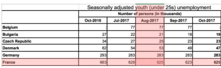
Figure 1: Sample dataset on French youth unemployment. RDF data extracted from the INSEE statistics INSEE publishes a set D of datasetsD1, D2, . . . etc. where each dataset Diconsists of
Searching for Truth in a Database of Statistics Tien-Duc Cao, Ioana Manolescu, and Xavier Tannier
a table (HTML table or a spreadsheet file), a titleDi.t and optionally an outlineDi.o. The title is a short nominal phrase stating what Di contains, e.g., “Seasonally adjusted youth (under 25s) unemploy-ment” in Figure 1. The outline, when present, is a short paragraph on the Web page from whereDi can be downloaded. The outline extends the title with more details about the nature of the statis-tic numbers, the interpretation of each dimension, methodological details of how numbers were aggregated etc.
A dataset consists of header cells and data cells. Data cells and header cells each have attributes indicating their position (column and row) and their value. For instance, in Figure 1, “Belgium”, “Bulgaria” etc. up to “France”, “Oct-2016” to “Oct-2017”, and the two fused cells above them, are header cells, while the other are data cells. Each data cell has a closest header cell on its column, and another one on its row; these capture the dimension values corresponding to a data cell.
To enable linking the results with existing (RDF) datasets and on-tologies, we extract the table contents into an RDF graph. We create an RDF class for each entity type, and assign an URI to each entity instance, e.g., dataset, table, cell, outline etc. Each relationship is similarly represented by a resource described by the entity instances participating to the relationship, together with their respective roles. System architecture A scraper collects the Web pages publicly accessible from a statistic institute Web site; Excel and HTML tables are identified, traversed, and converted into RDF graphs as explained above. The resulting RDF data is stored in the Apache Jena TDB server2, and used to answer keyword queries as we explain next.
3
SEARCH PROBLEM AND ALGORITHM
Given a keyword-based query, we focus on returning a ranked list of candidate answers, ordered in the decreasing likelihood that they contain (or can be used to compute) the query result. A relevant can-didate answer can be a data cell, a data row, column or even an entire dataset. For example, consider the query “youth unemployment in France in August 2017”. An Eurostat dataset3is a good candidate answer to this query, since, as shown in Figure 1, it contains one data cell, at the intersection of the France row with the Aug-2017 column. Now, if one changes the query to ask for “youth unemployment in France in 2017”, no single data cell can be returned; instead, all the cells on the France row qualify. Finally, a dataset containing 2017 French unemployment statistics over the general population (not just youth) meets some of the search criteria (2017, France, unemployment) and thus may deserve to appear in the ranked list of results, depending on the availability of better results.
This task requires the development of specific novel methods, bor-rowing ideas from traditional IR, but following a new methodology. This is because our task is very specific: we are searching for infor-mation not within text, but within tables, which moreover are not flat, first normal form database relations (for which many keyword search algorithms have been proposed since [6]), but partially nested tables, in particular due to the hierarchical nature of the headers, as we explained previously. While most of the reasoning performed by our algorithm follows the two-dimensional layout of data in columns
2https://jena.apache.org/documentation/tdb/index.html
3
http://ec.europa.eu/eurostat/statistics-explained/images/8/82/Extra_tables_Statis-tics_explained-30-11-2017.xlsx
and tables, bringing the data in RDF: (i) puts a set of interesting, high-value data sources within reach of developers and (ii) allows us to query across nested headers using regular path queries expressed in SPARQL (as we explain in Section 3.5).
We describe our algorithms for finding such answers below.
3.1
Dataset search
The first problem we consider is: given a keyword queryQ consisting of a set of keywordsu1,u2, . . .,um and an integerk, find the k datasets most relevant for the query (we explain how we evaluate this relevance below).
We view each dataset as a table containing a title, possibly a comment, a set of header cells (row header cells and column header cells) and a set of data cells, the latter containing numeric data4. At query time, we transform the queryQ into a set of of keywords W = w1, w2, . . . , wn using the method described in Section 3.2. Offline, this method is also used to transform each dataset’s text to words and we compute the score of each word with respect to a dataset, as described in Section 3.3. Then, based on the word-dataset score andW , we estimate datasets’ relevance to the query as we explain in Section 3.4.
3.2
Text processing
Given a textt (appearing in a title, comment, or header cell of the dataset, or the text consisting of the set of words in the queryQ), we convert it into a set of words using the following process:
• First,t is tokenized (separated into distinct words) using the KEA5tokenizers. Subsequently, each multi-word French lo-cation found int that is listed in Geonames6, is put together in a single token.
• Each token (word) is converted to lowercase, stop words are removed, as well as French accents which complicate matching.
• Each word is mapped into a word2vec vector [9], using the gensim [10] tool. Bigrams and trigrams are considered fol-lowing [9]. We had trained the word2vec model on a general-domain French news web page corpus.
3.3
Word-dataset score
For each dataset extracted from the statistic database, we compute a score characterizing its semantic content. A first observation is that datasets should be returned not only when they contain the exact words present in the query, but also if they contain very closely related ones. For example, a dataset titled “Duration of marriage” could be a good match for the query “Average time between mar-riage and divorce” because of the similarity between “duration” and “time”. To this effect, we rely on word2vec [9] which provides simi-lar words for any word in its vocabusimi-lary: if a wordw appears in a datasetD, and w is similar to w′, we considerw′also appears inD. The scorescore(w) of a dataset D w.r.t the query word w is 1 if w appears in D. .
4This assumption is backed by an overwhelming majority of cases given
the nature of statistic data. We did encounter some counterexamples, e.g. http://ec.europa.eu/eurostat/cache/metadata/Annexes/mips_sa_esms_an1.xls. However, these are very few and thus we do not take them into account in our approach.
5https://github.com/boudinfl/kea 6http://www.geonames.org/
Ifw does not appear in D:
• If there exists a wordw′, from the list of top-50 similar words ofw according to word2vec, which appears in D, then score(w) is the similarity between w and w′. If there are several suchw′, we consider the one most similar tow. • Ifw is the name of a Geonames place we can’t apply the
above scoring approach because “comparable” places (e.g., cities such as Paris and London) will have high similarity in the word2vec space. As the result, when user asks for “unemployment rate Paris”, the data of London might be returned instead of Paris’s. Letp be the number of places that Geonames’ hierarchy API7returns forw (p is determined by Geonames and depends onw). For instance, when querying the API with Paris, we obtain the list Île-de-France, France, Europe. Letwi′be the place at positioni, 1 ≤ i ≤ p in this list of returned places, such thatwi′appears inD. Then, we assign toD a score for w equal to (p + 1 −i)/(p + 1), that is, the most similar place according to Geonames has rankp/(p + 1), and the least similar has the rank1/(p + 1). If D contains several of the places from thew’s hierarchy, we assign to D a score forw corresponding to the highest-ranked such place. •0 otherwise.
Based on the notion of word similarity defined above, we will write w ≺ W to denote that the word w from dataset D either belongs to the query setW , or is close to a word in W . Observe that, by definition, for anyw ≺ W , we have score(w) > 0.
We also keep track of the location(s) (title, header and/or com-ment) in which a word appears in a dataset; this information will be used when answering queries, as described in Section 3.4. In summary, for each datasetD and word w ∈ D such that w ≺ W , we compute and store tuples of the form:
(w, score(w), location(w, D), D)
wherelocation(w, D) ∈ {T, HR, HC, C} indicates where w appears in D: T denotes the title, HR denotes a row header cell, HC denotes a column header cell, and C denotes an occurrence in a comment.
These tuples are encoded in JSON and stored in a set of files; each file contains the scores for one word (or bigram)w, and all the datasets.
3.4
Relevance score function
Content-based relevance score function. This function, denoted д1(D,W ), quantifies the interest of dataset D for the word set W ; it is computed based on the tuples(w, score(w), location(w, D), D) wherew ≺ W .
We experimented with many score functions that give high rank-ing to datasets that have many matchrank-ing keywords (see details in section 4.2.2). These functions are monotonous in the score ofD with respect to each individual wordw. This enables us to apply Fagin’s threshold algorithm [4] to efficiently determine thek datasets having the highestд1score for the queryW .
Location-aware score components. The location – title (T), row or column headers (HR or HC), or comments (C) – where a keyword occurs in a dataset can also be used to assess the dataset relevance.
7http://www.geonames.org/export/place-hierarchy.html
For example, a keyword appearing in the title often signals a dataset more relevant for the search than if the keyword appears in a com-ment. We exploit this observation to pre-filter the datasets for which we compute exact scores, as follows.
We run the TA algorithm using the score functionд1to select r × k datasets, where r is an integer larger than 1. For each dataset thus retrieved, we compute a second, refined score functionд2(see below), which also accounts for the locations in which keywords appear in the datasets; the answer to the query will consists of the top-k datasets according to д2.
The second score functionд2(D,W ) is computed as follows. Let w′be a word appearing at a locationloc ∈ {T, HR, HC, C} such that w′≺W . We denote by w′
loc,D(or justwloc′ whenD is clear from the context) the existence of one or several located occurrence ofw′ inD in loc. Thus, for instance, if “youth” appears twice in the title ofD and once in a row header, this leads to two located occurrences, namely youthT,Dand youthHR,D.
Then, forloc ∈ {T, HR, HC, C} we introduce a coefficient αloc allowing us to calibrate the weight (importance) of keyword occur-rences in locationloc. To quantify D’s relevance for W due to its loc occurrences, we define a location score componentfloc(D,W ). In particular, we have experimented with twoflocfunctions:
• flocsum(D,W ) = α P
w ≺Wscor e (wl oc, D)
loc
• floccount(D,W ) = αloccount {w ≺W }
where forscore(wloc,D) we use the value score(w), the score of D with respect to w (Section 3.3). Thus, each floc “boosts” the relevance scores of allloc occurrences by a certain exponential formula, whose relative importance is controlled byαloc.
Further, the relevance of a dataset increases if different query keywords appear in different header locations, that is, some in HR (header rows) and some in HC (header columns). In such cases, the data cells at the intersection of the respective rows and columns may provide very precise answers to the query, as illustrated in Figure 1: here, “France” is present in HC while “youth” and “17” appear in HR. To reflect this, we introduce another functionfH(D,W ) computed on the scores of all unique located occurrences from row or column headers; we also experimented with the two variants, fHsum and fHcountintroduced above.
Putting it all together, we compute the content- and location-aware relevance score of a dataset forW as:
д2(D,W ) = д1(D,W ) + Σloc ∈{T,HR,HC,C}floc(D,W ) + fH(D,W ) Finally, we also experimented with another functionд∗(D,W ) defined as: д∗ 2(D,W ) = д2(D,W ), if fT(D,W ) > 0 0, otherwise д∗
2discards datasets having no relevant keyword in the title. This is due to the observation that statistic dataset titles are typically carefully chosen to describe the dataset; if no query keyword can be connected to it, the dataset is very likely not relevant.
3.5
Data cell search
We now consider the problem of identifying the data cell(s) (or the data rows/columns) that can give the most precise answer to the user query.
Searching for Truth in a Database of Statistics Tien-Duc Cao, Ioana Manolescu, and Xavier Tannier
Such an answer may consist of exactly one data cell. For example, for the query “unemployment rate in Paris”, a very good answer would be a data cellDr,cwhose closest row header cell contains “unemployment rate” and whose closest column header cell contains “Paris”. Alternatively, query keywords may occur not in the closest column header cell ofDr,c but in another header cell that is its ancestor inD. For instance, in Figure 1, let Dr,c be the data cell at the intersection of the Aug-17 column with the France row: the word “youth” occurs in an ancestor of the Aug-17 header cell, and “youth” clearly characterizesDr,c’s content. We say the closest (row and column) header cells ofDr,cand all their ancestor header cells characterizeDr,c.
Another valid answer to the “unemployment rate in Paris” query would be a whole data row (or a whole column) whose header contains “unemployment” and “Paris”. We consider this to be less relevant than a single data cell answer, as it is less precise.
We term data cell answer an answer consisting of either a data cell, or a row or column; below, we describe how we identify such answers.
We identify data cells answers from a given datasetD as follows. Recall that all located occurrences inD, and in particular those of the formwHRandwHCforw ≺ W , have been pre-computed; each such occurrence corresponds either to a header rowr or to a header columnc. For each data cell Dr,c, we define#(r, c) as the number of unique wordsw ≺ W occurring in the header cells characterizing Dr,c. Data cells inD may be characterized by:
(1) Some header cells containing HR occurrences (for somew ≺ W ), and some others containing HC occurrences;
(2) Only header cells with HR occurrences (or only header cells with HC ones).
Observe that ifD holds both cell answers (case 1) and row- or column answers (case 2), by definition, they occur in different rows and columns. Our returned data cell answers fromD are:
• If there are cells in case 1, then each of them is a data cell answer fromD, and we return cell(s) with highest #(r, c) values.
• Only if there are no such cells but there are some relevant rows or columns (case 2), we return the one(s) with highest #(r, c) values. This is motivated by the intuition that if D has a specific, one-cell answer, it is unlikely thatD also holds a less specific, yet relevant one.
Concretely, we compute the#(r, c) values based on the (word, score, location, dataset) tuples we extract (Section 3.3). We rely on SPARQL 1.1 [14] queries on the RDF representation of our datasets (Section 2) to identify the cell or row/column answer(s) from each D. SPARQL 1.1 features property paths, akin to regular expressions; we use them to identify all the header cells characterizing a given Dr,c.
Note that this method yields only one element (cell, row or col-umn) from each datasetD, or several elements if they have the exact same score. An alternative would have been to allow returning sev-eral elements from each dataset; then, one needs to decide how to collate (inter-rank) scores of different elements identified in differ-ent datasets. We consider that this alternative would increase the complexity of our approach, for unclear benefits: the user experience is often better when results from the same dataset are aggregated together, rather than considered as independent. Suggesting several
data cells per dataset is then more a question of result visualization than one pertaining to the search method.
4
EVALUATION
This section describes our experimental evaluation. Section 4.1 de-scribes the dataset and query workload we used, which was split into a development set (on which we tuned our score functions) and a test set (on which we measured the performance of our algorithms). It also specifies how we built a “gold-standard” set of answers against which our algorithms were evaluated. Section 4.2 details the choice of parameters for the score functions.
4.1
Datasets and Queries
We have developed our system in Python (61 classes and 4071 lines). Crawling the INSEE Web site, we extracted information out of 19,984 HTML tables and 91,161 spreadsheets, out of which we built a Linked Open Data corpus of 945 millions RDF triples.
We collected all the articles published online by the fact-checking team “Les Décodeurs”,8a fact-checking and data journalism team of Le Monde, France’s leading national newspaper, between March 10th and August 2nd, 2014; there were 3,041 articles. From these, we selected 75 articles whose fact-checks were backed by INSEE data; these all contain links tohttps://www.insee.fr. By reading these articles and visiting their referenced INSEE dataset, we identified a set of 55 natural language queries which the journalists could have asked a system like ours.9
We experimented with a total of 288 variants of theд2function: •д1was eitherд1a,д1borд1c;
•д2relied either onflocsumor onfloccount; for each of these, we tried different value combinations for the coefficientsαT,αHC, αHRandαC;
• we used either theд2formula, or itsд2∗variant.
We built a gold-standard reference to this query set as follows. We ran each queryq through our dataset search algorithm for each of the 288д2functions, asking fork = 20 most relevant datasets. We built the union of all the answers thus obtained forq and assessed the relevance of each dataset as either0 (not relevant), 1 (“partially relevant” which means user could find some related information to answer their query) or2 (“highly relevant” which means user could find the exact answer for their query); a Web front-end was built to facilitate this process.
4.2
Experiments
We specify our evaluation metric (Section 4.2.1), then describe how we tuned the parameters of our score function, and the results of our experiments focused on the quality of the returned results (Sec-tion 4.2.2). Last but not least, we put them into the perspective of a comparison with the baselines which existed prior to our work: IN-SEE’s own search system, and plain Google search (Section 4.2.3).
8http://www.lemonde.fr/les-decodeurs/
9This was not actually the case; our system was developed after these articles were
Figure 2: Screen shot of our search tool. In this example, the second result is a full column; clicking on “Tous les résultats” (all results) renders all the cells from that column.
4.2.1 Evaluation Metric. We evaluated the quality of the an-swers of our runs and of the baseline systems by their mean average precision (MAP10), widely used for evaluating ranked lists of results.
MAP is traditionally defined based on a binary relevance judg-ment (relevant or irrelevant in our case). We experijudg-mented with the two possibilities:
•MAPhis the mean average precision where only highly rele-vant datasets are considered as relerele-vant
•MAPpis the mean average precision where both partially and highly relevant datasets are considered relevant.
4.2.2 Parameter Estimation and Results. We experimented with the following flavors of theд1function :
•д1b(D,W ) = 10 P w ≺W scor e (w ) •д1d(D,W ) = 10count {w ≺W } •д1f(D,W ) = P w ≺W10 scor e (w )
We also experimented with some modified variants that take into account the sum of matching keywords:
•д1c(D,W ) = P w ≺Wscore(w) + д1b(D,W ) •д1e(D,W ) = P w ≺Wscore(w) + д1d(D,W ) •д1д(D,W ) = P w ≺Wscore(w) + д1f(D,W )
A randomly selected development set of 29 queries has been used to select the best values for the 7 parameters of our system :αT, αC,αHR,αHC,αH, as well as the different versions ofд1andд2. For this purpose, we ran a grid search with different values of these parameters, selected among {3, 5, 7, 8, 10}, on the development query set, and applied the combination obtaining the best MAP results on the test set (composed of the remaining 26 queries).
We found that a same score function has lead to the bestMAPh andthe bestMAPpon the development query set. In terms of the no-tations introduced in Section 3.4, this best-performing score function is obtained by:
• Usingд1,c;
• Using fsum and the coefficient valuesαT = 10, αC = 3, αHR= 5, αHC= 5 and αH= 7;
• Using theд2∗variant, which discards datasets lacking matches in the title.
On the test set, this function has lead to MAPp= 0.76 and MAPh= 0.70 .
10https://en.wikipedia.org/wiki/Information_retrieval#Mean_average_precision
Figure 3:MAP results on the development set for 288 variants of the score function.
Dev. set 29 queries Dev. set 17 queries
MAPp 0.82 0.83
MAPh 0.78 0.80
Table 1: Results on the first and second development set.
Given that our test query set was relatively small, we performed two more experiments aiming at testing the robustness of the param-eter selection on the development set:
• We used a randomly selected subset of 17 queries among the 29 development queries, and used it as a new development set. The best score function for this new development set was the same; further, the MAP results on the two development sets are very similar (see Table 1).
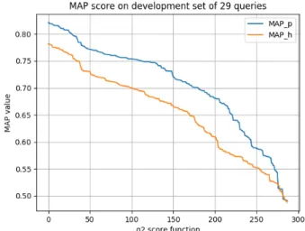
• We computed the MAP scores obtained on the full develop-ment set for all 288 combinations of parameters, and plotted them from the best to the worst (Figure 3; due to the way we plot the data, twoMAPhandMAPpvalues shown on the same vertical line may not correspond to the same score function). The figure shows that the best-performing 15 combinations leads to scores higher than0.80, indicating that any of these could be used with pretty good results.
These two results tend to show that we can consider our results as stable, despite the relatively small size of the query set.
Searching for Truth in a Database of Statistics Tien-Duc Cao, Ioana Manolescu, and Xavier Tannier
Running time. Processing and indexing the words (close to those) appearing in the datasets took approximately three hours. We ran our experiments on a machine with 126GB RAM and 40 CPUs Intel(R) Xeon(R) E5-2640 v4 @ 2.40GHz. The average query evaluation time over the 55 queries we identified is 0.218 seconds.
Our system INSEE search Google search
MAPp 0.76 0.57 0.76
MAPh 0.70 0.46 0.69
Table 2: Comparing our system against baselines.
4.2.3 Comparison against Baselines. To put our results into perspective, we also computed the MAP scores of our test query set on the two baselines available prior to our work: INSEE’s own dataset search system11, and Google search instructed to look only within the INSEE web site. Similarly to the evaluation process of our system, for each query we selected the first 20 elements returned by these systems and manually evaluated each dataset’s relevance to the given query. Table 2 depicts the MAP results thus obtained, compared against those of our system. Google’s MAP is very close to ours; while our work is obviously not placed as a rival of Google in general, we view this as validating the quality of our results with (much!) smaller computational efforts. Further, our work follows a white-box approach, whereas it is well known that the top results returned by Google are increasingly due to other factors beyond the original PageRank [2] information, and may vary in time and/or with result personalization, Google’s own A/B testing etc.
We end this comparison with two remarks. (i) Our evaluation was made on INSEE data alone due to the institute’s extensive database on which fact-checking articles were written, from which we derived our test queries. However, as stated before, our approach could be easily adapted to other statistic Web sites, as we only need the ability to crawl the tables from the Web site. As is the case for INSEE, this method may be more robust than using the category-driven navigation or the search feature built in the Web site publishing the statistic information. (ii) Our system, based on a fine-granularity modeling of the data from statistic tables, is the only one capable of returning cell-level answers (Section 3.5). We show such answers to the users together with the header cells characterizing them, so that users can immediately appreciate their accuracy (as in Figure 2).
5
RELATED WORK AND PERSPECTIVES
In this work, we focused on how to improving the usability statistic tables (HTML tables or spreadsheets) as reference data sources against which claims can be fact-checked. Other works focused on building textual reference data source from general claims [1, 8], congressional debates [12] or tweets [11].
Some works focused on exploiting the data in HTML and spread-sheet tables found on the Web. Tschirschnitz et al. [13] focused on detecting the semantic relations that hold between millions of Web tables, for instance detecting so-called inclusion dependencies (when the values of a column in one table are included in the values of a column in another table). Closest to our work, M. Kohlhase et
11Available at https://insee.fr
al. [7] built a search engine for finding and accessing spreadsheets by their formulae. This is less of an issue for the tables we focus on, as they contain plain numbers and not formulas.
Google’s Fusion Tables work [5] focuses on storing, querying and visualizing tabular data, however, it does not tackle keyword search with a tabular semantics as we do. Google has also issued Google Tables as a working product12. In March 2018, we tried to use it for some sample queries we addressed in this paper, but the results we obtained were of lower quality (some were irrelevant). We believe this may be due to Google’s focus on data available on the Web, whereas we focus on very high-quality data curated by INSEE experts, but which needed our work to be easily searchable.
Currently, our software is not capable of aggregating information, e.g., if one asks for unemployed people from all departements within a region, we are not capable of summing these numbers up into the number corresponding to the region. This could be addressed in future work which could focus on applying OLAP-style operations of drill-down or roll-up to further process the information we extract from the INSEE datasets.
REFERENCES
[1] R. Bar-Haim, I. Bhattacharya, F. Dinuzzo, A. Saha, and N. Slonim. 2017. Stance Classification of Context-Dependent Claims. In EACL. pages 251–261. [2] S. Brin and L. Page. 1998. The Anatomy of a Large-Scale Hypertextual Web
Search Engine. Computer Networks 30, 1-7 (1998), 107–117.
[3] T.D. Cao, I. Manolescu, and X. Tannier. 2017. Extracting Linked Data from Statistic Spreadsheets. In Proceedings of The International Workshop on Semantic Big Data.
[4] R. Fagin, A. Lotem, and M. Naor. 2003. Optimal Aggregation Algorithms for Middleware. J. Comput. Syst. Sci. 66, 4 (June 2003), pages 614–656. [5] H. Gonzalez, A. Halevy, C. Jensen, A. Langen, J. Madhavan, R. Shapley, and W.
Shen. 2010. Google Fusion Tables: Data Management, Integration, and Collabora-tion in the Cloud. In SOCC.
[6] V. Hristidis and Y. Papakonstantinou. 2002. DISCOVER: Keyword Search in Relational Databases. In Very Large Databases Conference (VLDB). 670–681. [7] M. Kohlhase, C. Prodescu, and C. Liguda. 2013. XLSearch: A Search Engine for
Spreadsheets. EuSpRIG (2013).
[8] R. Levy, Y. Bilu, D. Hershcovich, E. Aharoni, and N. Slonim. 2014. Context Dependent Claim Detection. COLING, pages 1489–1500.
[9] T. Mikolov, I. Sutskever, K. Chen, G.S. Corrado, and J. Dean. 2013. Distributed Representations of Words and Phrases and their Compositionality. In NIPS. pages 3111–3119.
[10] ˇR. Radim and S. Petr. 2010. Software Framework for Topic Modelling with Large Corpora. In Proceedings of the LREC 2010 Workshop on New Challenges for NLP Frameworks. pages 45–50.
[11] A. Rajadesingan and H. Liu. 2014. Identifying Users with Opposing Opinions in Twitter Debates. In International Conference on Social Computing, Behavioral-Cultural Modeling and Prediction. pages 153–160.
[12] M. Thomas, B. Pang, and L. Lee. 2006. Get out the vote: Determining support or opposition from Congressional floor-debate transcripts. In EMNLP. 327–335. [13] F. Tschirschnitz, T. Papenbrock, and F. Naumann. 2017. Detecting Inclusion
Dependencies on Very Many Tables. ACM Trans. Database Syst. (2017), pages 18:1–18:29.
[14] W3C. [n. d.]. SPARQL Protocol and RDF Query Language. https://www.w3.org/ TR/sparql11-query/. ([n. d.]).
[15] W3C. 2014. Best Practices for Publishing Linked Data. https://www.w3.org/TR/ld-bp/. (2014).