An integral multi-domain DPN operator as acceleration tool for the method of characteristics in unstructured meshes

HAL Id: cea-02361013

https://hal-cea.archives-ouvertes.fr/cea-02361013

Submitted on 20 Nov 2019

HAL is a multi-disciplinary open access

archive for the deposit and dissemination of sci-entific research documents, whether they are pub-lished or not. The documents may come from teaching and research institutions in France or abroad, or from public or private research centers.

L’archive ouverte pluridisciplinaire HAL, est destinée au dépôt et à la diffusion de documents scientifiques de niveau recherche, publiés ou non, émanant des établissements d’enseignement et de recherche français ou étrangers, des laboratoires publics ou privés.

An integral multi-domain DPN operator as acceleration

tool for the method of characteristics in unstructured

meshes

Simone Santandrea

To cite this version:

Simone Santandrea. An integral multi-domain DPN operator as acceleration tool for the method of characteristics in unstructured meshes. Nuclear Science and Engineering, Academic Press, 2006, 155 (2), pp.223-235. �10.13182/NSE155-223�. �cea-02361013�

AN INTEGRAL MULTI-DOMAIN DP

N

OPERATOR AS ACCELERATION TOOL FOR

THE METHOD OF CHARACTERISTICS IN UNSTRUCTURED MESHES

Simone Santandrea

Commissariat à l’Energie Atomique Direction de l’Energie Nucléaire

Services d’Etudes de Réacteurs et de Mathématiques Appliquées CEA de Saclay, DM2S/SERMA

91191 Gif-sur-Yvette cedex, France

simone.santandrea@cea.fr

Total number of pages : 29 Number of figures : 2 Number of tables : 3

ABSTRACT

The paper presents the recent developments of the acceleration techniques for the Method Of Characteristics (MOC) in the code APOLLO2. The main contribution concerns the introduction of a multi-domain DPN technique where all regions belonging to the same macro-domain are coupled by an integral

operator that is strictly equivalent to the MOC. Different macro-domains are coupled via currents that are defined with the DPN formalism. This new Integral DPN (IDPN) operator is build by using transmission and

escape probabilities factors that respect symmetries/anti-symmetries and complementary properties that are enforced to preserve the physics of the problem and to save computational effort. These factors are computed using the numerical tracking of the MOC operator. The paper presents results on realistic assembly calculations that demonstrate the effectiveness of the IDPN operator as a synthetic acceleration tool.

1 INTRODUCTION

In this paper we introduce an evolution of the DPN operator currently used in the two dimensional

MOC module of the APOLLO2 code [1] (called TDT) to accelerate the free iterations for the MOC. [2,3,4,5,6] Much work has been dedicated in recent years to the theme of acceleration techniques for the MOC. The reason for all this interest is the capability of the MOC to solve unstructured geometry problems without using any homogenization procedure. As with every method that uses the source iteration algorithm, the MOC can be very slow for collision dominated problems. Therefore acceleration techniques are essential in order to permit a wider practical application of the MOC. The DPN method, originally introduced by

Sanchez and Chetaine [7], is the operator to be used in the framework of the synthetic acceleration procedure for TDT. Generalizations of this technique have been recently introduced in [8,9] to improve the physical approximations of the initial formulation and to speed up the solution procedure. Further improvements are presented here and results are shown to illustrate the speed up factors of the TDT code (which is currently used for industrial calculations as a flux solver of the APOLLO2 [1] code system).

The principal contribution of this paper is a new way of using the DPN acceleration. Much alike the

classical Interface Current (IC) [10] treatment of the Collision Probability Methods (CPM), we show that the MOC admits a similar Integral DPN (IDPN) treatment. In this approach one subdivides the system into

macro-domains in each of which one applies an integral formalism that does not introduce any supplementary approximation with respect to the MOC. The coupling between regions belonging to different macro-domains is done via interface DPN currents that result from some simplifying assumptions on the

interface flux anisotropy. These assumptions are the only approximations of the method with respect to the MOC. One can expect this operator to behave better than the classic DPN operator, where the DPN

approximations were made at the interfaces between every region and not only at the interfaces between macro-domains. The main differences with respect to the standard IC method are that our method is not based on the CPM but on the MOC, that the interface approximations are given by the DPN method and that

the resulting equations have a response-matrix form that is different from that of the IC one. Since the numerical derivation of the IDPN method is consistent with the MOC, one can expect that this method will be

a good acceleration tool. We have not investigated, as it has been done for the IC method, the behavior of the IDPN method as a stand-alone operator. Only its capability as a means to accelerate the MOC free iterations

is considered here. Moreover, even if the IDPN method theory is valid also for three dimensional

unstructured geometries, our practical implementations are limited to two dimensional systems, due to the actual capabilities of TDT.

The paper is organized as follows. In section 2 we recall the basis of the MOC and introduce some notation for the following sections. In section 3 the IDPN synthetic operator is introduced and its detailed

properties are discussed together with the computational algorithm. In section 4 the external synthetic acceleration is revised and discussed. Section 5 is devoted to the analysis and discussion of results of calculations for a realistic assembly. Conclusions follow. Appendix A and B are dedicated to the description of improvements for the treatment of the equations for the boundary conditions, and to show many symmetries/anti-symmetries and reciprocity relations of the IDPN. We also demonstrate that this operator is

robust in the limit of nearly voided media.

2

THE METHOD OF CHARACTERISTICS

The DPN acceleration equations are used as a low-order operator for the acceleration of the MOC.

[7,8,9] The equations are obtained by the same projective technique that is used to derive the transport MOC equations but over different representation functions. We present here the transport MOC equations and in the next section the low-order DPN equations. Details can be found in [11,12].

The method of characteristics provides an iterative solution for the discrete ordinate formulation of the transport equation in a domain composed of unstructured homogeneous regions. The MOC equations are based on two approximations. The first consists of introducing a region-based flat spatial representation for the source term :

(

,

)

( )

s i i, i

q

r

Ω

∼

A

Ω

⋅ Σ

_⎣

⎡

φ

+

S

_⎦

⎤

,

r

∈

cell ,i

(1)

where A

( )

Ω =

{

Aρ

( )

Ω

}

is a vector of real spherical harmonics, s i, diag

{ }

s i, ρ

Σ = Σ contains for each region

the scattering coefficients associated to each spherical harmonic and

S

_i denotes the external source. The

components of vector

φ

i are the angular flux moments

( ) ( )

(4 )

1

,

4

i

d

A

π

φ

π

=

∫

Ω

Ω

ψ

i

Ω

(2) 4

where is the region averaged angular flux. All angular integrals are calculated with the discrete-ordinates quadrature formula.

( )

i

ψ

Ω

The second approximation is to use an expansion for the angular flux on region boundaries. For unstructured meshes one uses a set of parallel trajectories for each discrete ordinate direction Ω. The angular flux in direction Ω is then assumed to be constant over the cross sectional area associated with each trajectory,

(

,

)

t

( ) (

t ,

)

, t z z

ψ

θ

_⊥

ψ

Ω = +

∑

r Ω ∼ r Ω r r_⊥ Ω, (3)

and it is computed analytically along the trajectory. In this formula z and

r

_⊥ are, respectively, the coordinate in direction Ω and the coordinates over a plane orthogonal to Ω and

θ

_t

( )

r

_⊥ is the characteristic function associated to the cross sectional area of trajectory t.

The MOC equations comprise a balance equation and a transmission equation. Only the latter concerns us here. The transmission equation, which results from the analytical integration along each trajectory, gives the angular flux exiting the trajectory in terms of the incoming value and of the internal source. The homogeneity of the region as well as the flat source approximation are used to obtain:

( ) ( ) ( ) ( ) ( 1) , , ( )

1

( )

i i

( )

i i

( ),

i i R t R t n n n i i i i E R

e

t

e

t

q

ψ

−Σ

ψ

−Σ −

Ω

+ − Σ

−

=

+

Σ

(4)

where n is the iteration index, Ri(t) is the length of trajectory t within region i and Ω its direction.

A transport iteration consists of a sweep over all the trajectories crossing the domain. This provides the fluxes leaving the domain and, via use of the region balance equations, the updated values of the region averaged angular fluxes. The latter are then used in equation (2) to update the region averaged flux moments that are compared to the previous ones to check convergence. If the iteration has not converged, the sources are updated via Eq. (1) and the transport iteration is repeated. Details of the full MOC equations can be found in [2,12].

3

THE INTEGRAL DP

N

SYNTHETIC OPERATOR

A technique similar to the MOC is used to derive the DPN acceleration equations but with

approximations (1) and (3) replaced by low-order ones. The source region expansion is as in (1) but with a 5

smaller number of angular moments. The second approximation is more severe. The region boundary is decomposed into surfaces, a surface α being typically the common interface with a neighboring region, and a spatially constant angular approximation is assumed for the boundary fluxes:

( )

( , )

_s

A

_α

,

_s

S

_α

,

ψ

_±

r

Ω

∼

Ω

ψ

±

r

∈

(5)

where

S

_αstands for a generic surface and

ψ

_α± indicates exiting (+) or entering (-) surface averaged angular

moments. The vector

A

( )

Ω

contains all the spherical harmonic of polar order

k

≤

N

. The index “N” indicates that a “Double PN” spherical harmonics expansion is used in (5) (one per side), this gives its name

to the acceleration. Together with equation (5) the following currents are defined:

(2 )

( )

( , )

_s

,

S

J

dS

d

n A

A

α ρ ρ α υ π

ψ

Ω Ω

Ω

Ω

± ± ± ± ±

=

ρυ υ α

ψ

α

=

∑

∫

∫

i

r

(6)

where coefficient A are defined below in (9). We note that for the lowest moment this quantity is exactly the neutron current.

The first equation type of the DPN synthetic method expresses the current exiting a surface α in

function of the interface fluxes of neighboring regions. This is done by using the same set of tracking trajectories used for the MOC. In the standard DPN, method approximation (5) is applied to the surfaces of

all regions for all entering fluxes. This allows writing a transmission equation that couples all

ψ

_±,α quantities. In this work we consider a partition of the system into macro-domains composed of homogeneous regions and we apply (5) to only the surfaces between macro-domains. We use the integral transport equation over a given trajectory “t”. The angular flux exiting a region contained in macro-domain I is:

(

)

( , ) , 1 j j ij, i ex i j I j i j q e τ e τ e τ

ψ

+ − ∂

ψ

− − − ∈ < = + − Σ

∑

(7)

where τ(i,∂) is the optical length between the boundary of the macro-domain I and the entering boundary of region i along trajectory t, τj the optical length over a region j, Σj the total cross section in region j and τij the

optical distance between the entering point in region i and the exiting point of region j. Here we consider a point as “exiting” or “entering” with respect to the given trajectory. Figure 1 gives a sketch of the situation. Using the projection defined in (6) over an arbitrary surface, and applying the DPN approximation (1) to the

macro-domain interface entering fluxes, gives:

, , , , i i I i I J_αρ T_{α β}ρυ _βυ E_αρυ qυ T υ β υ

ψ

ψ

+ + − − + − ∈∂ ∈ =

∑

+

∑

= +E q (8)

where the source qυi has been defined implicitly in (1) and E and T are escape and transmission coefficients

respectively. The sum over β is done on region surfaces that belong to the surface ∂I of the macro-domain I,

and the sign “+/-” indicates that one has to consider the entering/exiting current. Equation (8) gives us an expression for all currents appearing in the system, regardless of their position with respect to macro-interfaces. The only approximation in (8) is to assume a reduced DPN flux anisotropy in the entering flux. In

order to allow coupling between macro-domains, another DPN expansion is assumed for the currents exiting

a macro-domain interface, that is to say:

,

J

_αρ

A

_αρυ _α

υ

ψ

+

=

∑

+ υ₊. (8a)

The definitions and properties of the coefficients A,E and T are quite similar to those of the standard DPN

method but, in order to stress some important differences, we recall them here. The matrix coefficients Aα

appearing in (6) and (8a), the transmission and escape coefficients in equation (8), are:

( ) ( )

(2 ) 1 , 4 A_αρυ dS d n Aρ Aυ α π π Ω Ω Ω Ω + + =

∫ ∫

⋅

( ) ( )

( ) ( )

,( ) ( ) , ( ) 1 _, 4 1 _{( ),} 4 i i i i T dS d n A A e E dS d n A A e E ρ _αβ ρ _α τ ρυ υ α β α β α τ ρυ υ α α α π τ π Ω Ω Ω Ω Ω Ω Ω Ω + − − + + + − → − → = ⋅ = ⋅

∫

∫

∫

∫

(9)

where (β→α) (respectively (i→α)) indicates that the integration domain has to include only the trajectories going from surface β to surface α (respectively from region i to surface α), ταβ is the optical distance

between α and β, τα ,(i) is the optical distance along direction Ω between the exiting side from region “i” and

the surface α, and, finally, E(Ri) is defined in (4) has been used. It is important to note that for consistency all

these coefficients are computed using the MOC trajectories for the integral over surface α. Moreover it is easy to see that the coefficients T and E obey symmetries/anti-symmetries and complementary relations. By “complementary” relation we mean a relation that links the two set of coefficients (E and T). The symmetry/anti-symmetry relation for the T coefficients are:

,

T_{α β}ρυ+ − =T_{α β}υρ+ − =s s T_{υ ρ β α}ρυ+ − (10)

where sρ stands for the parity of the harmonic ρ. It is important to stress how (10) can be used to greatly

reduce the computational effort necessary to obtain the transmission coefficients. Actually, instead of computing the coefficients T by using (9) and sweeping over all angles, we strongly reduce the integration domain thanks to (10), and compute, sweeping the track, the following integrals:

( ) ( )

[ ] [ ] ( ) 0, 0, / 2 1 ˆ _, 4 T_{α β}ρυ dS d n Aρ Aυ e ταβ α β α ρ υ π π π + − − + − → ≤ ∈ × =

_∫

_∫

⋅ Ω Ω Ω Ω Ω (11)

where the conditions listed below the integral sign mean that we are considering only the lowest diagonal angular harmonics and the angular directions belonging to the first two octants. Thanks to (10) it is easy to see that:

ˆ ˆ _,

T_{α β}ρυ+ − =T_{α β}ρυ+ − +s s T_{υ ρ β α}ρυ+ − (11a)

for ρ<υ, while for ρ>υ the transmission terms are obtained directly from (10). Calculations made with (11) imply the use of less than half of the trajectories that would be needed were we to use (9). A set of complementary relations are also valid for the escape coefficients:

(

)

, , [ i i I I i Eαρυ Tα βρυ Tα βρυ β β Tα βρυ α βAρυ β δ δ δ Σ + + + + − _{∉∂ ∈∂} + − ∈ =

∑

− − + _α+]. (12)

Equation (12) expresses the escape coefficients from a region “i” through a surface α as a sum over all the surfaces of the region. Three terms inside the sum must be distinguished. The first one, in which appears the symbol

δ

_β∉∂I , comes from the surfaces that are completely internal to the macro-region I. The second one has to be included when the boundary surface β belongs to the border of the macro-region I. The last one has to be considered when β coincides with α. Expression (12) gives the escape coefficients only in terms of the transmission ones. Therefore, the transmission coefficients are the only quantities directly computed from tracking.

Equation (8) must be completed to include the boundary conditions, that is to say, by expressing the entering boundary currents in terms of the exiting ones. A detailed description of these equations can be found in [11]. In this paper we introduce an important improvement for the boundary currents equations that is detailed in appendix A. This treatment is common to both the standard DPN and IDPN methods.

Since the source q contains flux moments, supplementary equations are needed to close the problem. These are obtained from the DPN region balance relations [9]:

(

)

, . i i i i i i J J _V V B υ υ α α q ρ ρυ υ α υ υ

φ

+ − − + = Σ Σ

∑

∑

(13)

Here B is an operator that takes into account the lack of numerical orthogonality for the spherical harmonic functions and is defined as:

( ) ( )

( )4 1 Ω . 4 Bρυ d Aρ Aυ π

π

=

∫

Ω Ω (13a)

Equation (13) becomes ill-conditioned for voided or weakly absorbent regions and is therefore cast into a more stable form. The algebraic manipulations are parallel to the ones used in the standard DPN

method [9], but many substantial differences appear due to the full coupling of the fluxes for regions belonging to the same macro-region. Another benefit of the procedure is to reduce the size of the problem to be solved iteratively. In fact, the iteration problem then deals only with the surface currents.

Substituting the expression (8) of the currents into formula (13), one obtains the following system per macro-region I :

,

I I I I I ext

M

φ

=

I

ψ

−

+

G q

(14)

where the expressions for matrices I, G, M are given in appendix B. It is important to note that the coefficients of the “incoming” matrix I can be directly obtained from the escape coefficients E given by (12), as detailed in equation (B2). This relation allows further computational savings. The matrix G of (14) is defined in (B3a) as G= BV − E,

Σ where the operator E can be defined as a function of the transmission

factors as showed in (B5), and B is the matrix (13a). An analytical definition of the operator G is given in appendix B (formulas (B7) and (B7a)), and there we show also that this operator is well defined also for nearly voided media. Moreover we also prove that:

ij ij ji

G

ρυ

=

G

υρ

=

s G s

ρ ρυ υ. (15)

Equation (15) enables us to reduce the computational effort by adopting a strategy similar to the one sketched in (11) and (11a) for the transmission factors.

The numerical counterpart of (B7) and (B7a) in the framework of the MOC is straightforward, and it is the way we have chosen to compute the operator E. The other possibility to compute EI, the escape matrix

for a given macro-region I, is described in appendix B, and makes use of reciprocity relationships between EI

and the transmission factors between all surfaces of I. We have opted for the first way since the storage required by EI is by far lower than the one required by the transmission factors. System (14) is then used to

express the flux moments as:

ˆ

ˆ

_,

ext

I

Gq

φ

₌

ψ

−

₊

_(14a)

where ˆI M I= −1 and . These expressions are inserted back into the transmission equation (8) through the source term (1). This gives:

1

ˆ

G

=

M G

−

(

)

(

)

1

ˆ

1

ˆ

s s d ext

A

T

E

I

A E

G

I

q

ψ

+

₌

−

_{+ Σ}

ψ

−

₊

−

_Σ

₊

_{, (16)}

where Σ =_{s i,} diag

{ }

Σ_{s i}ρ_, and Id is the identity matrix. It is worth noting that the matrix T+EΣsÎ, that appears

in (16), is sign-symmetric (as shown in appendix B), a property that is exploited to reduce the computational effort. Equation (16) is the final iterative form used to solve the problem and, since it is written for currents between macro-regions, it has a reduced dimension with respect to the standard DPN method. This means

that problem (16) should be faster to solve than its equivalent in the standard DPN method. Once the currents

have been obtained by solving (16), volume fluxes are obtained using (14a).

All transmission and escape coefficients can be shown to be bounded. For the transmission coefficients, this fact is clear from their definition (9). On the contrary, to show boundedness for the escape coefficients, it is necessary to develop and implement numerically an asymptotic expansion of equation (12). In fact, it is clear that expression (12) is greatly ill-conditioned for nearly voided systems. This development is given in appendix B.

Problem (16) has the same response-matrix form as the standard DPN operator. In [9] it has been

shown that a numerous set of preconditioning and optimization techniques can be used for this problem. This is an important point for our acceleration technique since all previous work, done in the framework of the standard DPN operator, can be re-used for the IDPN acceleration.

All the geometry partitions that we have used in this article have been obtained by the Spectral Bisection Algorithm (SBA) [13], that is a standard way to compute domain decompositions.

4

EXTERNAL SYNTHETIC ACCELERATIONS

In this work we have also applied the new IDPN acceleration as a multigroup acceleration technique

to improve the rate of convergence in multigroup calculations. Until now, most of the work that has been done to accelerate the external iterations used some non-linear strategy, [6] some classical linear extrapolations (like the Chebyshev one) or some Krylov subspace techniques. [14] Recently, Suslov [15] proposed a linear algorithm using a mono-group synthetic operator in the external framework. We implemented this idea in APOLLO2 with slight modifications, and used the standard DPN and the new IDPN

operator to test its efficiency. In this section we describe the algorithm and discuss implementation details. The multigroup external equations are driven by fission and, written with the iteration index, read :

(

)

( , ) ( , 1) ( ( 1) 1 p j p j p d u p L H

ψ

H

ψ

F

ψ

λ

− − − = + −1) , (17) where L is the one-group transport operator, Hd _{is the group-to-group and slowing down scattering operator,}

Hu is the up-scattering operator and F is the fission operator. The upper index p denotes the external iteration

index, while j is the thermal iteration index. Denoting by Jtot the number of thermal iterations per external

sweep, it is assumed in (17) that

ψ

( )p =

ψ

(p J, tot)for every external iteration p. One can then write the

converged solution as ( ) (p j, ) (p j) f

ψ

∞ ₌

ψ

₊ , , (18) where

(

)

( ) F ( ) L H

ψ

ψ

λ

∞ − = ∞ . (19) We substitute formula (18) in (19), taking into account (17), to obtain:

(

)

( ) ( ) ( ) ( ) ( ) ( ) , 1 , , , 1 , p j p p j p j p j s u u p F L H f H f f H

ψ

F

ψ

ψ

λ

λ

λ

− − ⎛ ⎞ − = + + ∆ + _⎜⎜ − ⎝ ⎠⎟⎟ (20) where

_{∆ =}

ψ ψ

( , )p j

₋

ψ

( , 1)p j−

is the difference between two consecutive transport iterates. Moreover, λ is the new eigenvalue obtained as the result of the multigroup correction problem (20). Problem (20) is an eigenvalue problem but with the presence of an external inhomogeneous term. An accelerated external iteration consists of a free MOC external iteration followed by one synthetic multigroup solution correction

given by (20). This last problem is solved using once again the power iteration solution strategy, that is to say by fixing the terms coming from fission and compute a multigroup solution with the help of “j” thermal iterations. The new estimated eigenvalue for the next iteration is given by the usual condition:

( ) ( ) ( )

(

)

( ) ( )

(

)

, , , , , , p j p j k k p j p j k F f F f

ψ

λ

ψ

− + == + 1 ,

where the index k refers to the external iterations necessary to solve the problem (20).

5

RESULTS AND COMPARISONS

In this section we will prove the effectiveness of the IDPN acceleration, presenting some results

related to the Atrium Benchmark. [16] Here we will compute a version of this benchmark that makes use of a sixteen group P0 transport corrected cross section library that has been obtained by a previous self-shielding

phase in APOLLO2. [17] The Atrium benchmark is a severe realistic assembly calculation, that has strong transport effects and slow convergence rate. The spatial computational mesh used for our calculation is shown in figure 2, and it consists of 3560 regions. A full description of the case can be found in [16], and we here only insist on some basic features. The Atrium benchmark represents a BWR assembly. The fuel and gadolinium rods are surrounded by an external as well as an internal box, where homogeneous water flows. As it is typical for these reactors, liquid water concentration varies inside the assembly. In fact, for the considered version of the benchmark, we have a 0% vapor fraction inside both the internal and the external box of the assembly, while we have a 40% vapor fraction for the water in direct contact with fuel rods. Fuel rods are characterized by three different enrichments, and strong flux heterogeneities appear next to gadolinium rods, that are distinguishable in figure 2 by the very fine mesh refinement necessary to represent flux gradients. We used the transport code APOLLO2 where all the developments we present here are now implemented. The tracking data used to compute the benchmark are shown in table 1. We used a product angular formula with sixteen uniform azimutal angles, and two optimal Bickley polar angles. [18] The transversal spatial step is 0.025 cm. This results in a total of 643,617 horizontal intersections with computational regions.

A first comparison deals with two calculations that have used a DP1 or IDP1 multigroup initialization

and a thermal synthetic acceleration, a procedure that is also discussed in [9]. Table 2 gives the performances

of the old DP1 operator and of the new IDP1 one. Free iterations are also shown in order to illustrate the

efficiency of the acceleration methods. All the results in the table, with the exception of the free iterations ones, were obtained using a mesh grid that was constructed using the recursive SBA. [13] For the standard DP1 method, the chosen grid is used to make a two-level multigrid acceleration method [9], while for the

IDP1 operator we use this same grid to compute macro-domain integral probabilities. We have always used

the adapted ILU0 preconditioning technique [9] to speed up the DPN and IDPN equations. Due to their great

impact over the total computational time the building times are also shown. All computing times are expressed in seconds on a 2.8Ghz 512Kb cache PC.

Building times strongly depend on the preliminary manipulations required: algebraic elimination process for the standard DP1 method, and computation of the transmission probabilities for the IDP1 method.

As the number of regions per macro-region increases, the building time also increases, but the burden of the accelerated iterative resolution strongly decreases. Therefore the appropriate number of regions to be included in each macro-region should be optimized. This phenomenon was already described in [9] and we will not insist on it here. Our numerical tests show that a good number of regions per macro one for the Atrium benchmark is 70, so we always retained the grid mesh resulting from the recursive SBA with this fixed maximum number of regions. It is important to stress that, while for the standard DPN method the grid

mesh has no physical impact, for the IDPN it should be beneficial to take advantage of a “physical” grid, that

is a grid with reduced flux anisotropy on grid interfaces. This is the case for example for the classical IC method where the grid is given by the region decomposition of the assembly. In fact one can suppose that flux anisotropy is reduced at region interfaces. In this work we will always use the “numerical” grid given by the SBA, even if it certainly does not guarantee the best result.

As one can see from table 2, the best time with consistent tracking, 26.4 sec., is obtained for the IDP1

operator. The standard DP1 operator spends a lot of time in the initial building phase, and requires 151

internal transport iterations. In spite of the non-“physical” SBA grid mesh, the spectral behavior of the IDP1

operator is quite better since it converges with only 102 iterations. The thermal synthetic acceleration, used with the IDP1 method, reduces the number of total transport iterations by almost a factor of 40 with respect to

free iterations. Unfortunately, the IDP1 acceleration (as well as the DP1 one) requires an expensive building

phase that accounts for half of the total time; this explains why the accelerated calculation is only 15 times faster than the free iterations.

In order to reduce the expensive building phase, we introduced a low-order tracking described at the third row of table 1. The low-order tracking is now used to compute a synthetic IDP1 operator: this choice

entails a lower building cost but can cause a poorer convergence rate. If one compares the data for the reference and low-order tracking, one can see that the number of tracks that are used to build the IDP1

operator is now decreased by a factor of four with respect to the reference case. We will call this approach “inconsistent” since it is generally required that the acceleration operator be obtained in a “consistent” way with respect to transport, in order to avoid problems of poor convergence or even of divergence of the accelerated algorithm. Using an inconsistent acceleration can therefore lead to lack of robustness. At this time we do not suggest a method to prevent these drawbacks. In the results we show, and more generally on the basis of our experience, we can state that the behavior of the acceleration is not degraded too much if one maintains the low-order tracking formula at an acceptable level.

The new IDP1 results are given in fourth row of table 2. The use of a low-order tracking should entail

poorer IDP1 performances. The results in table 2 show that this effect is very limited, since the total number

of iterations goes from 102 to 107. On the contrary, thanks to the faster building time, the total computational time decreases from 26.4 to 23.6 seconds. Note that while most of the IDP1 building time is directly

proportional to tracking, the standard DP1 building time strongly depends on the geometrical structure of the

problem, and weakly on tracking. The use of a low-order tracking has practically no effect on the standard DP1 operator, and therefore we do not present inconsistent DP1 results in table 2.

A last batch of results (table 3) deals with the impact of the external synthetic acceleration. We used this algorithm in conjunction with the standard DPN operator or the new IDPN operator. Both have been

computed inconsistently with respect to transport: we used the low-order tracking described by the third row of table 1. In table 3, one can see that the external acceleration is very effective for the synthetic IDP1

operator, since it reduces the total number of internal transport iterations from 106 to 48. Unfortunately this yields only a slight time reduction, the total computational time goes from 23 to 22.3 seconds. This is due to the fact that the synthetic external acceleration “transfers” a great amount of work from the transport to the synthetic operator. And in fact the total number of synthetic operator problems to be solved is multiplied by more than a factor two, with respect to the cases presented in table 2.

The only possibility to further reduce the computational time is to solve the IDPN problem faster,

without increasing building times. We suppose that this could be possible by adopting a full multilevel algorithm (and not a purely two-level one as in this paper). We will address this issue in future works.

6 CONCLUSIONS

In this paper a new DPN synthetic operator has been introduced. Its main approximation consists in

supposing reduced flux anisotropy over a limited number of surfaces. In fact, after having subdivided the system into some macro-regions, the IDPN operator supposes limited flux anisotropy only over those

surfaces that divide macro-regions. Thanks to this preliminary hypothesis, and by making use of the basic MOC equations, one can find an integral operator whose unknowns are the flux components over macro-interfaces. Many symmetries/anti-symmetries and complementary relations help to minimize the computational effort, and taking into account important physical properties in the numerical operator. Calculations made with APOLLO2 on the Atrium Benchmark show that the IDP1 method is more efficient

than its standard counterpart, and that it can be retained as an efficient acceleration tool. The preliminary time necessary to build the operator is reduced and the spectral performance is improved. The behavior of the new IDPN operator in conjunction with the external synthetic acceleration approach has also been

evaluated. Even if the overall computational time is reduced, further improvements of the IDPN operator are

necessary to make this reduction significant. In particular, we suggest adopting a true multilevel algorithm that will help to reduce building and solution times. We will address this issue in future works.

APPENDIX A: BOUNDARY CONDITIONS TREATMENT

In this section we give a detailed description of the boundary current treatment. The complete form of the boundary current equations has been given elsewhere. [8] What we describe here is an improvement in the treatment of these equations for the DPN problem. We shall show that for all local boundary conditions

(i.e. all boundary conditions where the neutrons exiting the system re-enter through the same surface), exiting currents can be eliminated from the iterative part of the problem with almost no computational and memory cost. Let us write the transmission problem (8) in the following manner:

i i T T E S

ψ

ψ

ψ

ψ

βψ

+ − − ∂ ∂ − + ∂ ∂ ⎧ = + + ⎪ ⎨ = ⎪⎩ , (A1) 15

where we have distinguished the transmission contributions coming from internal currents “

ψ

−” and from external currents “

ψ

_∂−” . Each entering external current can be written as

( ) t α α

ψ

−

₌

βψ

+ S . (A2) For local boundary conditions t(α)=α, but in general surfaces do not coincide. For both cases equation (A1)

can be re-written as i i T T E

ψ

+

ψ

−

ψ

+ ∂ ∂ = + + (A3)

where T_∂ =T_∂

β

. The system of equations (A3) is a reduced form of the initial system (A1): it contains less

unknowns and equations but shares the same profile for the remaining equations. This means that contrarily to standard elimination processes, where fill-in always appears, here no elements are added to the initial operator. In the case of no local boundary conditions, the further elimination of the boundary exiting currents appearing in (A3) would cause fill-in and, for this reason, we decided not to eliminate them. For local boundary conditions the situation is different. In fact one can extract the boundary external currents from (A3), and write them as

( ) ( ) ( , ) ( ) ( ) , i i i j j i j i T T , E q

ψ

_{∂ +}

ψ

_{− ∂}

ψ

_{∂ +} ≠ = +

∑

+ , (A4) where

ψ

( )_,i

∂ + is the outgoing external modes related to the i-th external surface, T(i) is the transmission matrix

giving the contribution of internal currents to the i-th external boundary current, is the transmission matrix describing the link between the j-th external surface and the i-th one and describes the escape. It is clear that the only case when is different from zero is when the i-th and the j-th surface share the same region. For convenience we will suppress from now on the tilde notation over the T

( , )i j T_∂ ( )i

E q

( , )i j T_∂ ∂ symbol since

each external transmission term will always be post-multiplied by the albedo operator. The objective is to

show that building the formal inversion

1 ( , ) , i j i j

I

T

− ∂

⎛

⎞

−

⎜

⎝

∑

⎠

⎟

is not computationally expensive and can be done

without any fill-in in the LU decomposition necessary to compute this inverse. To see this, let us eliminate the first external current from the system (A4), to obtain

(

)

1 ( ,1) (1, ) ( ) ( ) ( ,1) (1) ( ,1) (1, ) ( , ) ( ) ( ) ( ,1) (1) , , 1 i i i i i i i j i j j i i j i j D

I

T

_∂

T

_∂

ψ

_{∂ +}

T

T

_∂

T

ψ

₋

T

_∂

T

_∂

T

_∂

ψ

_{∂ +}

E

T

_∂

E

q

≠ >

⎡

⎤

⎡

⎤

⎡

−

=

_⎣

+

_⎦

+

∑

_⎣

+

_⎦

+

_⎣

+

_⎤⎦

, (A5) which is valid for all i>1. Rearranging these equations to a unit diagonal gives:

( ) ( ) ( , ) ( ) ( ) , 1 ,1 , 1 1 , i i i j j i j i j T T E q i 1

ψ

_{∂ +}

ψ

_{− ∂}

ψ

_{∂ +} ≠ > = +

∑

+ ∀ > , (A6) where , ( )

( )

₁ 1

(

( ) ( ) ( )_{,1 1}

)

1 i i i i

T

=

D

−

T

+

T

_∂

T

T

_∂( )_,1i j,

=

( )

D

_i1 −1

(

T

_∂( ) ( )i,1

T

_∂1,j

+

T

_∂( )i j,

)

and ₁( )i

( )

1 1

(

( )i ( ) ( )i,1 1

)

i

E

=

D

−

E

+

T

_∂

E

.

System (A6) is formally similar to system (A4), with the exception that the number of unknowns is reduced by one in all equations but the first, and that the profile of the operator has been correspondingly reduced since each coupling term due to the first external current has been eliminated from all equations. A similar reasoning can be applied to all the other currents, so that at the final step one obtains an upper diagonal operator. Before the l-th step one has to eliminate the l-th current from the equations greater than l. After the elimination of this current from the i-th equation of the system (where clearly i>l) this equation reads ( ) ( ) ( , ) ( ) ( ) , , , i i i j j l l j i j l T T E_li q

ψ

_{∂ +}

ψ

_{− ∂}

ψ

_{∂ +} ≠ > = +

∑

+ (A7)

where, after defining l ( ) ( )i l, l i, i

D

= −

I

T

_∂

T

_∂ , one has ( )

( )

1

(

( ) ( ) ( )_, 1 , 1 1 i l i i l i l l l

T

=

D

−

T

₋

+

T

_{∂ −}l

T

₋l

)

, 1l ∂ − , (A8a)

( )

1 ( )_, ( , ) , i j i j l l i T_∂ = D − T . (A8b)

Equations (A8a-b) allow the calculation of all matrices ( )i l

T

from all matrices at the preceding step ( ( )i₁ l

T

₋ ). As before, the elimination process gives rise only to the cancellation of boundary terms, without any fill-in. The remaining step is to complete the inversion of the original ( , )

,

i j i j

I−

∑

T_∂ matrix by substituting back, from

the last until the first, the new computed equations. Let us call Nbd the total number of boundary equations in

(A4). After the Nbd steps described above, one has an upper diagonal operator where the last equation gives

the Nbd -th external current in function only of internal unknowns and collision sources. The

back-substitution of this equation into the (Nbd -1)-th one allows again to express the (Nbd -1)-th external current in

function only of internal currents and collision sources.

This back-substitution process can be easily repeated, until each external current is expressed in function only of internal currents and collision sources. In fact when treating the j-th equation in the backward procedure, one can use the following situation:

( ) ( ) ( , ) ( ) ( ) , , , ( ) ( ) ( ) , , , j j j k k j j i k j i i i i back i back

T

T

E

j

q

for i

j

T

E

q

ψ

ψ

ψ

ψ

ψ

∂ + − ∂ ∂ + > ∂ + −

=

+

+

>

=

+

∑

(A9)

where one can note that all equations beyond the j-th one have already been diagonalised. The back-substitution of these equations into the j-th one gives:

( ) ( ) , , ( ) ( ) ( , ) ( ) ( ) ( , ) ( ) , , , , , j j j back j back j j j i i j j i i j i i back j i i back i j i j T E

T

T

T

E

T

E

Vq

ψ

_{∂ + ∂}

ψ

_{− ∂} > >

⎡

⎤

⎡

=

_⎢

+

_⎥

+

_⎢

+

⎣

∑

⎦

⎣

∑

⎤

⎥

⎦

,

which gives the recursive definition of the back matrices. Finally the system (A4) is reduced to a system of the form: ( ) ( ) ( ) , i i i back back

T

E

q

ψ

_{∂ +}

=

ψ

₋

+

, (A10)

where all external elements have disappeared. Eqs (A10) are substituted into (A4) to completely eliminate the boundary currents from the problem and finally obtain:

, (

(

)

(

i back back

T

T T

T E

E

)

)q

ψ

+ + ∂ −

ψ

+ ∂ ∂ − ∂ ∂ ∂

=

+

∑

+

∑

+

,

where the sums over is done on boundary currents. The balance equations have also to be consistently modified. In fact the original balance equations (15a), written without the hat sign, can be split in the following manner:

∂

H

GVq

H

H

GV

φ

ψ

−

βψ

+

ψ

− ∂ ∂

=

+

=

+

+

q

)

, (A11) where H∂ stands for the boundary part of the balance operator H. By making use of (A10) one obtains:

(

_H

_T

ˆ

_H

) (

_G

_H

_{E Vq}

ˆ

φ

β

ψ

−

β

∂ ∂

=

+

+

+

,

where and Tˆ Eˆare the transmission and escape operators appearing in (A10).

APPENDIX B: MATRIX COEFFICIENTS OF THE INTEGRAL DP

N

METHOD AND

ASYMPTOTIC LIMITS OF ESCAPE PROBABILITIES

In this appendix we give some numerical details about the DPN equations. First of all we detail the

expression of matrices M, G and H appearing in (14). Next we consider the vacuum limit for the escape coefficients in equation (9).

Substituting (8) into (13) yields:

(

, ,

)

(

, ,

)

, , , , , ,

if

,

if

.

j j j I j I j j I j I

T

T

E

E

q

J

J

T

A

E

q

I

ρυ ρυ υ ρυ ρυ υ α β α β β α α β υ υ ρ ρ α α _{ρυ υ ρυ υ ρυ υ} α β β α α α β υ υ υ

ψ

α

ψ

ψ

α

+ − − − − + − + − + − − − − + ∈∂ ∈ ∈∂ ∈

⎧

₋

₊

₋

⎪

−

_{= ⎨}

−

+

∈∂

⎪

⎩

∑

∑

∑

∑

∑

I

∉∂

(B1)

From equation (B1) we derive the following expression for the leakage term of the balance equation:

(

)

(

)

( )

(

)

( ) , , , , , , , , , , ,

1

1

I i I ij I I i i I i i I I _{j j} I _j i i I i E

J

J

T

T

T

A

E

E

E

q

ρυ β ρυ ρ ρ α α ρυ ρυ ρυ ρυ α _{α β α β} α _{α β} αβ _α υ_β α β υ α ρυ ρυ ρυ α _{α α} α _α α

δ

δ

δ

δ

δ

ψ

+ − + − − + − + + − ∉∂ ∈∂ ∈ ∈∂ ∈ ∉∂ ∈∂ ∈ ∈

−

⎧

_⎡

_⎤

⎫

=

_⎨

_⎣

−

+

−

_⎦

_⎬

Σ

_⎩

Σ

_⎭

⎧

_⎡

_⎤

⎫

+

_⎨

_⎣

−

+

_⎦

_⎬

Σ

⎩

⎭

∑

∑

∑

∑

,

.

j j I υ υ ∈

∑

− (B2)

Equation (B2) implicitly defines the matrix I of equation (15), and another auxiliary matrix EI used to

construct the matrices G and M of equation (14). The incoming matrix I can be better re-written in function of the escape coefficients (12):

(

)

(

)

(

)

(

)

, , , , , , , 1 1 , I I i i i I I i i i I T T T A s s T T T A s s E ρυ ρυ ρυ ρυ ρυ α α αβ β α β α β α β α α , ρ υ ρυ ρυ ρυ ρυ ρ υ ρυ α β α β α α β α αβ α β α

δ

δ

δ

δ

δ

δ

− + − − − + − − + − + + + − + + ∉∂ ∈∂ ∈ ∉∂ ∈∂ ∈ ⎡ ⎤ = − _⎣ − + − _⎦= Σ ⎡ ⎤ − _⎣ − + − _⎦= Σ

∑

∑

− (B3)

where (10) has been used together with the fact that A_αρυ+ =s s Aρ υ _αρυ− . (B3) represents a complementary

property between the coefficients of the incoming matrix I and escape coefficients E. Re-inserting (B1) into the balance equation (13), one obtains the following expression for the matrix MI of equation (15) :

( )

[

( )

, j _] I ij i ij I ij ij s j i B V M V E ρυ ρυ ρυ _υ ρυ δ δ δ = + − Σ Σ , (B4) 19

where i,jŒI. Finally, the matrix G that appears in (15) is given by: , I I i BV G = − Σ E (B4a)

where EI is defined in (B1) and B in (13). Equations (B3) and (10) allow us to show that the matrix T+EΣsÎ

appearing in (16) is sign-symmetric that is to say that it satisfies the relation t

(

T + ΣE _sIˆ

) (

=s T+ ΣE _sI sˆ

)

.

Indeed, first note that (B3) and (10) can be written in matrix form as t _{and . Moreover let}

us suppose that (and then also

T =sTs t

E

= − s

sI

1

I I

M

Σ

−

Σ

_I

M

_I−1) is sign-symmetric. This implies that

(

1

) (

t

s I s I

T+ ΣE M I− =s T + ΣE M I s−1

)

, (B5)

which is the expected result. We still need to demonstrate that

M

_I

Σ

_I−1 is sign-symmetric. This can equivalently be shown for EI (thanks to (B4)). Therefore, inserting the definition of E_αρυ_i given by (12) inside

the expression (B2) of EI , one obtains:

(

)

(

)

(

(

)

, , , , , , , , , [ ]. ij j I I i j I I I I I I I E T T T T T T T T A A T ρυ ρυ ρυ ρυ ρυ α β _{α β α β α β α β} α β ρυ ρυ ρυ ρυ α β α β α β α β α β α β ρυ ρυ ρυ α αβ α α α β α β

δ

δ

δ

δ

δ

δ

δ

δ

δ

δ

+ + + − − − − + − − + − + + + − + − + − ∉∂ ∉∂ ∈ ∈ ∉∂ ∈∂ ∈∂ ∉∂ ∉∂ ∈∂ ∈∂ Σ = − + − + − + − − −

∑

)

(B6)

Interchanging i with j in the left hand side amounts to interchanging α with β in the right hand side.

Using (10), one then sees that each term in (B6) is transformed either into itself multiplied by sρsυ, as it is the

case for the terms into the third line of (B6), either in other terms of the same row multiplied by sρsυ, as it is

the case for the terms in the first two lines. We will find this result in another way in formula (B8). Equations (B4) and (B8) can be used to reduce the computational effort as well as the memory storage, since they show that only halves of the matrices EI and T+EΣsÎ have to be computed and stored.

Thanks to (B6) an analytical definition of operator G can be given:

( ) ( )

( , ) ( ) ( , ) 1 ( ) ( ) 4 lm s i i s j ij ij s l m l T r V j i V m T r V Gρυ Eρυ d dr n Aρ Aυ E

τ

e τ E

τ

i

π

− ∈ Ω ∩ → ∂ ∈ Ω ∩ = − =

∫

Ω

∫

Ω ⋅ Ω Ω

∑

≠ j.(B7)

In equation (B7) the symbol (j→i) stands for the angular directions going from region j to region i, the

symbol T(r,Ω) stands for the set of all the chords intersected by the trajectories that pass through the point r

with angle Ω, so that T(r,Ω)∩Vi (T(r,Ω)∩Vj) stands for the subset of chords that belong to region i (or region

j) and symbol E is defined in (4). Therefore the sum in (B7) takes into accounts the case of the intersections with non-convex regions. The optical chord lengths τl,τm and τlm are related respectively to the chord in

region i, to the chord in region j and to the distance between the exiting point of segment l and the entering point of segment m. An analogous expression can be written for the diagonal terms:

( ) ( )

(2 ) ( , ) , ( , ) 1 4 { [ ( )]/ ( ) ( ) }, i lm s i s i i ii ii s i V l i l m l T r V l m T r V l m B V G E dr d n A A l E E e E ρυ ρυ ρυ ρ υ π τ

π

τ

τ

+ ∂ − ∈ Ω ∩ ∈ Ω ∩ ≠ = − = Ω Ω ⋅ Ω Ω Σ − Σ +

∫

∫

∑

∑

i

τ

(B7a)

where the second sum inside parentheses comes again from non-convex regions. Inspecting (B7) and (B7a), one can readily realize the symmetric role of indexes i and j as well as of the angular indexes. This assures us that

ij ij ji

G

ρυ

=

G

υρ

=

s G s

ρ ρυ υ. (B8)

Next, we show that the escape coefficient for the source in Eq. (9) remains bounded at the vacuum limit. From the expression for E_αρυ_i we obtain

( ) ( )

( )

( )

0 1 lim 4 i i i i E_αρυ dS d Aρ Aυ R e ταβ O β α β α π − Σ → ∈ → →

∫

∑

∫

Ω Ω ⋅n Ω Ω _i + Σ , (B9) _i where we used 2

( )

2 0 1 lim 2 i i i R i i i i R e R O −Σ Σ → Σ − _{→ − + Σ}

Σ i . Formula (B9) shows that the escape coefficients

remain bounded, but unfortunately does not give any complementary relation. This means that, in case of nearly voided media a new integral, given by (B9), must be computed.

Another term that must be treated specifically at the vacuum limit is the diagonal term of operator G in equation (B3a). One can show that this diagonal term has the following limit

( ) ( )

( )

( )

0 2 2 ( , ) , ( , ) 1 lim 4 { [ / 2 ] ( ) ( ) i i lm s i s i ii V k i l m k T r V l m T r V l m G dS d A A l O E e E ρυ ρ υ π τ π τ τ + Σ → ∂ − ∈ Ω ∩ ∈ Ω ∩ ≠ → Ω Ω⋅ Ω Ω + Σ +

∫

∫

∑

∑

n i },

that is to be computed explicitly for the nearly voided cases. 21

REFERENCES

1. Sanchez, R., Mondot J., Stankovski, Z., Cossic, A., Zmijarevic, I., 1988. APOLLO II: A user-oriented, portable, modular code for multigroup transport assembly calculations. Nuclear Science and Engineering 100, 352-362.

2. Halsall, M.J., 1980. CACTUS, a Characteristics Solution to the Neutron Transport Equation in Complicated Geometries. AEEW-R 1291, Atomic Energy Establishment, Winfrith, Dorchester, Dorset, United Kingdom.

3. Smith, K., 2000. “CASMO-4 characteristic methods for two-dimensional PWR and BWR core calculations”. Transactions of the American Nuclear Society, 83, 294-296.

4. Dahmani M., R. Le Tellier, Roy R. and Hebert A., 2005. An efficient preconditioning technique using Krylov subspace methods for 3D characteristics solvers. Annals of Nuclear Energy 32, 876-896.

5. Hong S.G., Cho N.Z., 1998. CRX: a code for rectangular and hexagonal lattices based one the method of characteristics. Annals of Nuclear Energy 25 (8), 547-565.

6. Nam Zim Cho, 2005. Fundamentals and recent developments of reactor physics methods, Nuclear Engineering and Technology, 37, 25-78.

7. Sanchez, R., Chetaine, A., 2000. A Synthetic acceleration for a two dimensional characteristic method in unstructured meshes. Nuclear Science and Engineering 136, 122-139.

8. Santandrea S. and Sanchez R., 2002. Acceleration Techniques for the characteristics method in unstructured meshes. Annals of Nuclear Energy, 29, 323-352.

9. Santandrea S. and Sanchez R., 2005. Analysis and improvements of the DPN acceleration technique for

the method of characteristics in unstructured meshes. Annals of Nuclear Energy, 32, 163-193.

10. Sanchez, R., Mao, L., 1997. New development in the Interface-Current Module TDT. Proc. Joint Int. Conf. Mtg. Mathematical Methods and Supercomputing for Nuclear Applications. Saratoga, New York, October 5-9, 1997, p. 29, American Nuclear Society.

11. Santandrea S., 2001. Qualification Physique et amélioration du schéma numérique d’une méthode des caractéristiques pour l’équation de transport des neutrons, PHD dissertation, Université d’Evry Val d’Essonne, France.

12. Sanchez, R., Mao, L., Santandrea S., 2002. Treatment of boundary condition in trajectory based deterministic transport methods. Nuclear Science and Engineering 140, 23-50.

13. Saad, Y., 1996. Iterative Methods for Sparse Linear Systems. PWS Publishing Company, Boston, Massachusetts.

14. Warsa J.S., Wareing T.A., Morel J.E. and McGhee J.M., 2004. Krylov Subspace Iterations for Deterministic k-Eigenvalue Calculations. Nuclear Science and Engineering, 147, 26-42.

15. Suslov, I., 2002. “An algebraic collapsing acceleration method for the acceleration of the inner (scattering) iterations in long characteristics transport theory”. Proceeding of the international conference on Supercomputing in Nuclear Application, (SNA 2003) Paris 22-24 September 2003.

16. AEN-NEA, Nuclear Energy Agency, OECD 2003. Physics of Plutonium Recycling. VolumeVII: BWR MOX Benchmark-Specification and Results.

17. Zmijarevic, I., 2005. Personal Communication.

18. Leonard, A., Mc Daniel, C.T., 1995. Optimal Polar Angles and Weights for the Characteristics Method. Transactions of the American Nuclear Society, 73, 172-173.

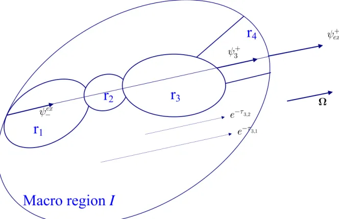
FIGURE 1

Figure 1: Sketch for the transport equation (7). The macro-region “I” contains many micro regions “r”. For a trajectory along direction Ω, many intersections

have to be considered from the entering to the exiting point. In order to express each exiting angular flux along this trajectory, the exponential of the optical length between these regions must be computed. For example, to express thanks to equation (7), a sum over the preceding collision sources (weighted

with and ) and over the entering flux must be done.

3 ψ+ 3,2

e

−τ

e

−τ3,1

ψ

+ ex

ψ

+ ex

ψ

₋

r

1

r

4

r

₃

r

₂

3

ψ

+ 3,2

e

−τ 3,1

e

−τ

Ω

Macro region I

24

FIGURE 2

Figure 2: Computational mesh for the BWR atrium assembly.

TABLE 1

trajectories tracks azimuthal angles polar angles Transversal

Integration step

162 643,617 16 (uniform) 2 (Bickley) 0.025cm

143 162,610 10 (uniform) 2 (Bickley) 0.05 cm

Table 1: Tracking parameters for the calculation of the Atrium assembly with cyclic trajectories. The number of tracks is the total number of intersections of trajectories with regions. The second and the third rows gives, respectively, the data of the reference tracking and of the DPN low-order one.

TABLE 2

building time Total time Nb. External it. Nb. Internal it. DP1 Consistent tracking 22.7 41.4 7 151 IDP1 Consistent tracking 12.8 26.4 5 102 IDP1 Inconsistent tracking 9.44 23.6 5 107 Free Iterations 412 13 3848

Table 2: Results for the Atrium assembly calculation using the standard DP1 operator and the new integral

IDP1 operator. All cases are DPN-initialized eigenvalue calculations. The computational times are expressed

in seconds. The reference k-effective is 1.13811.

TABLE 3

building time Total time Nb. External it. Nb. Internal it.

DP1 19.5 sec 40.3 6 96

IDP1 9.4 sec 22.3 3 48

Free Iterations 412 13 3848

Table 3: Results for the Atrium assembly calculation using the standard DP1 operator and the new integral

IDP1 operator with double tracking. All cases are DPN-initialized eigenvalue calculations and external

iterations are accelerated with the external synthetic algorithm. The computational times are expressed in seconds. The reference k-effective is 1.13811.

Figure Captions

Figure 1: Sketch for the transport equation (7). Macro-region “I” contains many micro regions “r”. For a trajectory along direction Ω many intersections have to be considered from the entering to the exiting point. In order to express each exiting angular flux along this trajectory the exponential of the optical length between these regions must be computed. For example to express thank to equation (7) a sum over the preceding collision sources, weighted with and , and over the entering flux must be done.

3

out

ψ

3,2

e

−τ

e

−τ3,1

Figure 2: Computational mesh for the BWR Atrium assembly.