HAL Id: hal-01617202
https://hal.archives-ouvertes.fr/hal-01617202
Submitted on 16 Oct 2017HAL is a multi-disciplinary open access
archive for the deposit and dissemination of sci-entific research documents, whether they are pub-lished or not. The documents may come from
L’archive ouverte pluridisciplinaire HAL, est destinée au dépôt et à la diffusion de documents scientifiques de niveau recherche, publiés ou non, émanant des établissements d’enseignement et de
A hybrid random walk method for the simulation of
coupled conduction and linearized radiation transfer at
local scale in porous media with opaque solid phases
Gérard L. Vignoles
To cite this version:
Gérard L. Vignoles. A hybrid random walk method for the simulation of coupled conduction and lin-earized radiation transfer at local scale in porous media with opaque solid phases. International Journal of Heat and Mass Transfer, Elsevier, 2016, 93, pp.707-719. �10.1016/j.ijheatmasstransfer.2015.10.056�. �hal-01617202�
“
A hybrid random walk method for the simulation of coupled conduction and
linearized radiation transfer at local scale in porous media with opaque solid
phases
”,
by
G. L. VIGNOLES,
published in
Int. J. of Heat & Mass Transfer (2016), vol. 93, pp. 707–719.
doi:10.1016/j.ijheatmasstransfer.2015.10.056
A hybrid random walk method for the simulation of
coupled conduction and linearized radiation transfer at
local scale in porous media with opaque solid phases
Gerard L. Vignoles1
University of Bordeaux,
Laboratoire des Composites ThermoStructuraux (LCTS) UMR 5801: CNRS-Herakles(Safran)-CEA-UBx
3, All´ee de La Bo´etie, 33600 Pessac, France Tel: (+33) 5 5684 3305
Abstract
Heat transfer properties from ambient up to extremely high temperatures are a key feature of advanced thermal protection and thermal exchange materials – like ce-ramic foams or fiber assemblies. Because of their porous nature, heat transfer rests not only on conduction in opaque solids and on convection in pores, but also on radiation trough pores. The precise knowledge of the thermal behavior of these materials in these conditions is an issue. In a ”virtual material” framework, we present a computational simulation tool for heat transfer in such materials, com-bining solid-phase conduction and linearized radiative transfer in open or closed radiating cavities with opaque interfaces. The software is suited to working in large 3D blocks as produced e. g. by X-ray CMT or by image synthesis. An origi-nal Monte-Carlo Mixed Random Walks scheme accounting for both di↵usion and radiation is presented and validated. The application to a real image of a fibrous medium is described and discussed, principally in terms of the influence of the di↵usion/radiation ratio on the e↵ective (large-scale) di↵usivity tensor.
Keywords: Radiative heat transfer ; Conductive heat transfer ; Numerical
method ; Virtual material Highlights
• New hybrid random-walk scheme for coupled conduction-radiation heat transfer
• Scheme validated with respect to analytical cases
• Works on large 3D domains like discretized X-ray CT blocks
• Fastest heat transfer direction changes between radiative and conductive modes
1. Introduction
Advanced thermostructural materials must be able to resist to mechanical and thermal loads at very high temperatures, while controlling heat transfer, bringing either thermal insulation, as in Thermal Protection Systems in atmospheric reentry of space objects [1, 2] or thermal transfer, as in Concentrated Solar Power plants [3]. Many porous materials have been and are still being developed for these purposes, like carbon and ceramic foams [4] and fibrous media [5].
One of the crucial points in the engineering of such materials is to determine their thermophysical properties. At elevated temperatures, transfers in the bulk of materials may include simultaneous contributions from conduction in the solid phase (fibre, matrix, interphase) and from radiation via the pore space [6]. While modeling of the conductive transfer via these materials is well developed [7, 8] things are not the same for the coupled conductive-radiative transfer. The analy-sis of the coupled transfer requires the use of adapted modeling tools that allow considering these di↵erent contributions. One of the fundamental problems is the disparity in nature of the two types of transport. On the one hand, the conductive
transport is of easy modeling using classical methods of PDE solutions, such as finite elements ; on the other hand, the radiative transfer obeys to quite distinct equations, such as RTE (Radiative Transfer Equation), from which the resolution can be envisaged in di↵erent ways: discrete ordinates [9] with a finite element resolution [10, 11], finite di↵erences with discretization of space directions [12], moments methods [13], Hottel zones method [14], etc . . . Classically, in the com-mercial codes of thermal calculation, the radiation in enclosed cavity is solved by the calculation of radiative exchanges between facets of a matrix (form factors) or by discrete ordinates. One of the most popular methods for the RTE resolution is ray tracing [15–20]; often rays are traced at random directions (Monte Carlo method)[6, 21–24]. The interest is double: first, the Monte Carlo method is well adapted for numerical integration of equations written in the 5-dimensional space of position/orientation; second, there is a natural interpretation of this method, be-cause it simulates more or less directly the propagation of IR rays. This method has been applied to the computerized representation of very complex 3D struc-tures [17–19], as it has very small memory requirements. Up to now, these meth-ods yield e↵ective radiative properties for materials; however, they have to be combined with another appropriate method giving the conductive behavior of the solid phase to build an e↵ective heat di↵usivity or conductivity in the coupled regime. The Monte Carlo Random Walk (MCRW) method is also used to de-scribe the phonon transfer in a material [25], similar to that of rare gas molecules in porous media [26, 27]. In such a case, a direct simulation of species transport (phonons or molecules) is performed. However, another random walk method can be used, which is the simulation of Brownian motion at a larger scale than that of the absorption length [28–30]: it is adapted to solve the energy equation or whatever similar elliptical equation (pressure equation for groundwater flow, mass di↵usion equation, etc), but in it the transported species is not any more the direct
simulation of an ”energy carrier”. An interesting advantage of this method is that it takes quite naturally into account the local media anisotropy. The present study proposes a method coupling the latter Brownian motion scheme in a solid with the above mentioned ray tracing technique in the radiative cavities of the opaque material, in a single mixed algorithm which provides a natural coupling between linearized radiation and conduction.
According to the nature of the studied material, the influence of radiative heat transfer on the value of its e↵ective properties is more or less marked. Hence, many studies have taken radiation into account in the description of foams which are subject to important radiative transfer, because of their high porosity. The contribution of radiation to the thermal properties has been evaluated for polymer [31, 32], carbon [33] and metal [19] foams.
Here, the specific need is to calculate, when radiation can be linearised, an e↵ective di↵usivity ae↵ and a thermal conductivity ke↵ of porous materials with
opaque and transparent phases, as full tensors, from 3D images obtained by X-ray Computerized Micro-Tomography (CMT), taking into account simultaneously conductive and radiative heat transport in the bulk of the material.
We will first describe the principle and implementation of the mixed random-walk method, then present its validation against analytical data; finally, an appli-cation to an actual 3D CMT image of a porous fibrous material will be shown and discussed.
2. Model and method 2.1. Principle
2.1.1. Problem frame
The heat transfer problem treated here concerns a heterogeneous domain con-taining two phases : the solid, subject to conduction, and the void, in which
ra-diation takes place. The solid phase is a grey body characterised by a di↵use reflection law and of emissivity ". All thermophysical properties of this phase (thermal conductivity ks, thermal di↵usivity as, density ⇢s, thermal capacity per
unit mass cp,s and emissivity " are uniform. The size of the domain is supposed
large enough to be representative of the whole material, i. e. it is a Representative Volume Element (RVE). We will assume that an average temperature hTi can be defined on this RVE. Actually, the temperature is not defined in the void phase, so that the average temperature in the usual sense has to be taken as the intrinsic solid-phase average hTsis.
The radiative flux per unit area at a point M (r) of an opaque gray wall with di↵usive emissivity " writes:
qrad = " Z ⇡ 2 0 Z 2⇡ 0 h I (T) Iin(✓, )icos ✓ sin ✓d✓d (1)
where I (T) is the equilibrium intensity at temperature T (r) and Iin(✓, ) the
inci-dent intensity depending on ✓, angle between the inciinci-dent unit vector and the unit normal to the wall, and , the azimuth. In a random walk method the summations over ✓ and are statistically achieved both for the emitted and absorbed fluxes per unit area.
The temperature field at time t at a point M (r) writes:
T (r, t) = Tref+ ˜T (r, t) (2)
where Trefis a reference temperature for the whole medium and ˜T is the
tempera-ture variation in M at time t. It is here assumed that the perturbations are small : ˜T/Tref<<1.
In this approximation, and considering constant thermophysical properties in the solid, the conducto-radiative heat transfer in the porous medium is fully lin-earized. Although this condition is not necessary in principle, it will be useful for an easy implementation into an MCRW scheme, described as follows.
2.1.2. Relation between enthalpy and walkers
The basic idea of the method, as for any Lagrangian scheme, is to translate temperature into walkers. The ithconductive walker located in an elementary dis-cretized volume element V around a point M (r) at time t generates a temperature variation equal to :
ˆTi(r, t) = H
⇢scp,s V (3)
where H (J/walker) is a ”quantum of excess enthalpy”. The temperature per-turbation field is then approximated by summing over all walkers present in the elementary volume V :
˜T (r, t) =X
i2 V
ˆTi(r, t) (4)
2.1.3. It¯o-Taylor Random Walk
For a simulation of heat di↵usion in a homogeneous, isotropic medium, a ran-dom walker may follow an It¯o -Taylor scheme [34], where, for fixed time intervals
tw, every di↵usive space step xdis computed as:
xd = p 2as tw 0 BBBBB BBBBB BBBBB @ 1 2 3 1 CCCCC CCCCC CCCCC A (5)
in which 1,2,3are random numbers obeying a Gaussian distribution with zero
mean and unit variance. This scheme has been extended to the case of hetero-geneous and anisotropic media [35], i.e. for which the di↵usion coefficient is tensorial and a function of space a
s(x): x =✓ div · as(x)◆ tw+ 0 BBBBB BBBBB BBBBB @ p as,11(x) 1 p as,22(x) 2 p as,33(x) 3 1 CCCCC CCCCC CCCCC A p 2 tw (6)
Developed for dispersion of solutes in underground aquifers[34], this scheme has also been validated when applied to the simulation of gas infiltration in porous media [30], a totally analogous problem.
2.1.4. Ray-tracing
As opposed to the random-walk scheme, heat transfer by radiation is simu-lated by Monte-Carlo ray-tracing [6]. Walkers are emitted by a surface with local temperature ˜T with an emission probability proportional to the emitted flux. Since the emission directions ⌦ obey Lambert’s law of di↵use emission (or reflection), their distribution is:
p (⌦) d⌦ = cos ✓d⌦ = cos ✓ sin ✓d✓d (7)
Here, it is not considered that a walker represents a single photon: the parameters of the emission rules are averages over the whole wavelength spectrum. This lim-itation could be easily removed, but the resulting computation of energy-resolved radiation would be much longer. After emission, a walker travels instantly along a straight line (i.e., a ray) until it meets another surface element, upon which it will be reflected with a probability equal to the reflectivity 1 " (since " and the ab-sorptivity ↵ are equal). The time is not advanced between an emission event and an absorption event, regardless of the number of intermediate reflection events. 2.1.5. Coupling conduction and radiation
The most crucial point is a correct specification of the coupling between both transfer modes, and it lies on the probability that a walker having arrived at the interface enter the void. Such a probability is not computed the same way, de-pending on the side of the interface the walker is coming from. If it arrives from the void space, then its computation is easy: it is exactly the material’s reflectivity 1 " = Pv!v. On the other hand, when it comes from the solid phase, a more original, though empirical, reasoning can be carried out.
When a conductive walker hits at point M a solid/void interface, it brings its energy quantum H during a time tw, shorter than the time step t of the method
– the latter being a time step used to quantify transient heat transfer – and has travelled a distance xwfrom the last di↵usion point. The corresponding incoming
flux is evaluated at the surface element S surrounding M as: qin(M, t) = H
tw S (8)
According to the It¯o-Taylor scheme, the average value of the squared displacement D
x2 d
E
is equal to 6as tw. Recalling eq. (3), one has :
qin(M, t) = k sˆT 6 VD x2 d E S (9)
Let us note that the ratio 6 V/ S between the volume and the surface elements associated to the walker is approximately the size of the random walk displace-ment step h| xd|i = q 8 3⇡ qD x2 d E
– i.e. one considers the volume element as a hemisphere with radius h| xd|i. Averaging the flux over all elementary events –
and consequently over all possible incoming directions, one has: D qinE(M, t) = ksˆT qD x2 d E2 p 2 p 3⇡ = ksˆT h| xd|i p 3⇡ 2p2 (10)
Actually, the length that appears in the denominator of eq. (10) may be somewhat shorter, because the trajectories are interrupted by the wall collision. We can therefore assume safely that:
D
qinE(M, t) = ksˆT
h| xw|i (11)
where h| xw|i is an average distance of the last step before reaching the wall, which
we expect to be comparable to the average random walk step size h| xd|i.
In Appendix A, it is found analytically that h| xw|i ⇡ 0.72 h| xd|i; on the
other hand, eq. (10) would give h| xw|i ⇡ 0.92 h| xd|i; numerically, the relation
is h| xw|i ⇡ 0.81
qD x2
d
E
Generally, only a fraction ofD qinEis emitted at M. The maximal emitted flux
per unit area associated to the walker writes, after linearization: d qe max = 4" T3 ref ⇡ ˆTd⌦ ecos ✓e (12)
In eq. (12), ˆT has been neglected as compared to Trefand I (Tref) = T
3 ref
⇡ is the
equilibrium intensity, d⌦eis the emission solid angle and ✓eis the angle between
the emission direction and the normal to the interfacial element. If the photon propagation is instantaneous, eq. (12) shows that the emitted energy during twis
limited. Summing over all directions we obtain : ⌦ qe
max↵=4" Tref3 ˆT (13)
The quantity defined here may be compared to the incoming average flux com-puted in eq. (10). Two cases have to be considered:
• If D qinE ⌦ qe
max↵, the walker is emitted without condition in the void.
The limitation of the flux is the due to conduction. • IfD qinE>⌦ qe
max↵, the emission probability is inferior to unity and is then
the ratio between the emitted flux and the incoming flux. To summarize, the global emission probability writes:
Ps!v(M, t) = 8 >>>>> < >>>>> : ⌦ qe max↵ h qini = 4" T3 refh| xw|i ks if ⌦ q e max↵< D qinE 1 if ⌦ qe max↵ D qinE (14) Note that the limitation due to the conduction appearing in the second case can be avoided by diminishing the time step, which will lower the average space step h| xd|i and the ”last step” size h| xw|i.
We can fairly well see that Ps!v is actually a ”numerical Nusselt number” based on the pseudo-heat transfer coefficient hbb = 4" Tref3 and the average step
2.2. Implementation
2.2.1. Single walk algorithm
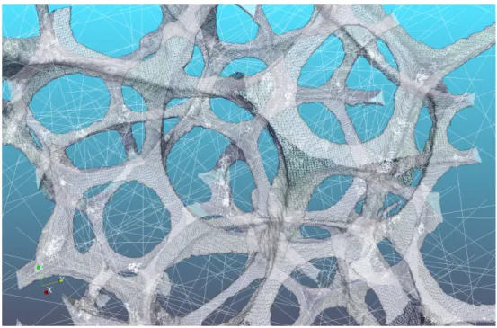
The proposed algorithm couples the classical ray-tracing method with Brown-ian motion in a hybrid random walk. Every excess enthalpy carrier will switch its behavior from one to the other walk routine depending whether it lies in the solid or in void space. Everytime it meets a surface element, it is decided whether it will continue its walk in the void or in the solid, using the probabilities Ps!vand Pv!vdefined above. Figure 1 is an illustration of a typical walk.
Figure 1: Rendering of a typical random walk in an open-cell foam.
2.2.2. Surface discretization
The position of the interface is obtained by the Simplified Marching Cube (SMC) technique [36]. This efficient scheme is a trade-o↵ between the full March-ing Cube (MC) algorithm, accurate but requirMarch-ing large memory storage space, and
a simple cubic voxel discretization, which is unable to approximate the interface surface area per unit volume [27]. However, in that scheme, it is unfortunately possible to obtain portions of solid phase slabs with zero thickness. This issue is solved using a procedure described in Appendix B.
2.2.3. Boundary conditions (BCs)
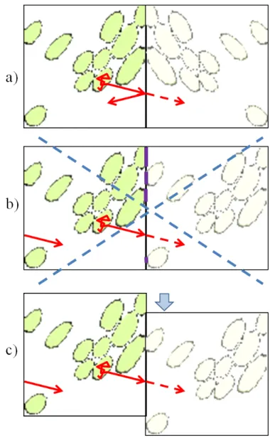
In homogenization or averaging techniques, periodicity or symmetry BCs are commonly employed, both with drawbacks. For instance, some material sam-ple domains, like those obtained by image processing from X-ray Computerized Tomography may not be naturally periodic, or display a texture with o↵-axis di-rections. In these cases, setting periodicity or symmetry BCs can severely a↵ect the results of the heat transfer computations. Using random walk schemes allow straightforwardly to implement less harmful BCs. The representation of a pe-riodicity BC would be the reintroduction of a walker in the opposite face of the resolution domain, i. e. applying a translation of exactly one cell edge vector to its ”local” coordinates, while keeping untouched ”global” coordinates. But it is easy to reintroduce the walker in the opposite face at a random location in the same phase, instead of at exactly the same location. This has the e↵ect of implementing an ”average periodicity” condition, i. e.:
hq (Lx)inx· nx = hq (0)inx· nx (15) hT (Lx)inx = hT (0)inx
where nx is the outward normal to the x = 0 face and inward normal to the
x = Lxface, and h•inxis the face-average of a quantity: h inx = 1 LyLz Z Ly 0 Z Lz 0 dydz (16)
Figure 2: Several boundary condition schemes: a) Symmetry (induces an artificial alignment of the e↵ective tensor eigenvalues on the image principal axes) , b) Translation (does not work on non-periodic images), c) Translation plus a random tangential movement of the replicated image.
If the two opposite faces do not have the same porosity, then the reintroduction of the walkers from the least porous face (with porosity ⇧ ) to the most porous one (⇧+) is biased by the porosity di↵erence, i. e. a random number between 0
and ⇧+ is drawn and if it is larger than ⇧ the walker is reflected back instead of
transferred to the opposite face. Failure to implement this correction would add an artificial global heat flux.
2.2.4. Obtaining an e↵ective di↵usivity by the displacement covariance
A classical method to derive the e↵ective di↵usion tensor from random walks statistics is to apply Einstein’s relationship [28, 37]:
a
comp =n!1t!1lim
h(x(t) x(0)) ⌦ (x(t) x(0))i
2t (17)
In practice, all random walkers are initially located in the image and are allowed to walk freely; when they encounter an image border, the above-mentioned bound-ary rules (either symmetry, periodicity, or average periodicity) are applied. Two coordinate sets are handled: a local one, always inside the image, and a global one, which is used for the computation of eq. (17). In the present case, one has to note that since all random walkers travel instantly through the void space, they are always found inside the solid when performing an evaluation of relation (17). Consequently, the obtained di↵usion tensor is an intrinsic solid average. The ef-fective di↵usion tensor, averaged over the whole material, is deduced by:
a
e↵=acomp(1 ⇧) (18)
where ⇧ is the pore (void) volume fraction. One has to note that Einstein’s rela-tionship only applies in the hypothesis of finite horizon in void space; in the con-verse case, the e↵ective di↵usion coefficient obtained by relations (17-18) slowly diverges with time [38]. Finally, since the heat capacity is always obtained by the
rule of mixtures, a
e↵and ke↵are related by:
k e↵ =ae↵. ⇣ ⇢cp ⌘ e↵ =ae↵. ⇣ ⇢cp ⌘ s(1 ⇧) (19)
2.2.5. Obtaining an e↵ective conductivity by flux/gradient correlation
To circumvent the above-mentioned problem, and to compare this approach with more classical averaging or homogenization techniques, a di↵erent compu-tational routine has been designed, inspired by the M¨uller-Plathe method [39] used in molecular dynamics to obtain the e↵ective thermal conductivity of a given solid or liquid by the flux/gradient correlation method. In this method, no double coordinate system (local/global) is required. While maintaining periodic, sym-metric or ”average-periodic” boundary conditions on two sets of opposite faces, we define a ”semi-permeable” wall boundary condition on the last pair of opposed faces: for instance, all walkers reaching the x = Lx face are allowed to re-enter
the image by the x = 0 side whereas all walkers reaching the x = 0 face are for-bidden to re-enter on the other side and simply undergo specular reflection. This has the e↵ect of creating a flux in the positive direction. As a consequence, the walker concentration acquires a gradient, with fewer walkers per unit volume on the ”permeable” side. The walker fluxes are acquired on the semi-permeable pair of faces, while the concentration gradient is recorded on all pairs of faces, and one line of the e↵ective inverse conductivity tensor is obtained:
⇣ k 1 e↵ ⌘ i j= D ˜T (Li) E ni D ˜T (0)Eni Ljhqinj · nj (20) The accuracy of numerical estimations of the concentration and of the flux may be enhanced by a time averaging technique. A limitation of this approach is that if the image is not symmetric in addition to periodic, then a severe bias is added to the concentration field with respect to what is expected from an averaging prob-lem, resulting in an inaccurate homogenization. Nonetheless, if the image is very
detailed (i. e. its size is much larger than the largest feature size), this bias has a negligible influence.
3. Validation
The method has been tested against cases for which analytical solutions are available: first, parallel plates separated by void space; then, a simple cubic array of void spheres dispersed in a conductive matrix. All walls are grey and di↵use, with a variable emissivity.
3.1. Parallel plates with grey di↵use walls
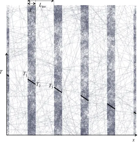
This simple case of a periodic medium is described in Figure 3: parallel solid plates with thickness L1are separated by void slices with thickness Ltot L1. The
void volume fraction is ⇧ = 1 L1/Ltot and the internal surface area per unit
volume is Sv = 2/Ltot. The temperature profile, for a positive horizontal heat
flux qx > 0 is sketched on the same figure. Evidently, the addition of thermal
resistances in series will give the e↵ective thermal resistance, as detailed hereafter. 3.1.1. Analytical model
The heat flux normal to the plates is expressed by Fourier’s law in the solid: qx= Lks
1⇣ ˜T2 ˜T1
⌘
(21) It is also expressed by the radiative exchange laws, under Rosseland’s linear ap-proximation:
qx = hbb
2 "⇣ ˜T3 ˜T2 ⌘
(22) where the 2 " denominator translates multi-reflection e↵ects [6].
The e↵ective conductivity is given by Fourier’s law over the whole unit cell: qx = ke↵
Ltot⇣ ˜T3 ˜T1
⌘
Figure 3: Periodic medium with parallel plates. Solid and void spaces are identified by the distinct nature of the random walk steps. A temperature profile T (x) is superimposed to the figure. Note that T has not to be defined in the void space.
Solving eqs. (21-23) for ke↵yields: 1 ke↵ = L1 Ltot ! 1 ks + 1 Ltot ! 2 " hbb ! (24) This relationship may be reinterpreted as :
1 ke↵ =(1 ⇧) 1 ks 1 + 2 " Nu ! (25) where a radiative Nusselt number has been defined as :
Nu = hbbL1 ks = hbb ks · 2 (1 ⇧) Sv (26)
Combining with eq. (19), the e↵ective di↵usivity will be given by: ae↵= as (1 ⇧)2 1 + 2 " Nu ! 1 (27) We note that there is a very simple relation between the Nusselt number and the solid-to-void transition probability:
Ps!v =Nuh| xw|i
L1 (28)
3.1.2. Numerical results and discussion
Computations have been carried out with several relative slab thicknesses, val-ues of the emissivity, of Ps!v, and of the step size h| xw|i. The M¨uller-Plathe-like
scheme has been applied, the walker concentration profiles recorded along the x coordinate, as well as the jx flux. The total number of random walkers was
N = 24000; the dimensionless time was ast/L2tot=6; every run has taken
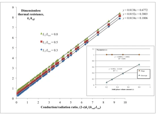
approx-imately 1 minute on a single 2-GHz Core i7 CPU with 1.3 GHz memory access frequency. Figure 4 is a plot of the dimensionless thermal resistance ks/ke↵against
the conduction/radiation ratio, expressed as ⇣2 " Ps!v
Lpix
Ltot ⌘
. Indeed, rewriting eq.(24) we can see straightforwardly that the former is an affine function of the latter :
ks ke↵ = L1 Ltot ! + 2 " Ps!v Lpix Ltot ! · h| xL w|i pix ! (29)
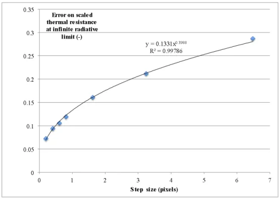
Therefore the slope of the obtained lines should be equal to the step size expressed in pixel units, and the intercept should be the relative solid volume amount. What is actually found is a slope in very close agreement with the dimensionless step size and a somewhat shifted intercept; the error between the actual intercept and the expected intercept decreases with diminishing stepsize as h| xw|i0.4, as
illus-trated by fig. 5.
Figure 4: Scaled thermal resistance for parallel plates for 3 di↵erent L1/Ltotratio, as a function of
the conduction/radiation ratio, for h| xw|i = 0.81 pixels. The inset gives the slopes and intercepts
as a function of the solid phase volume amount.
The same computations have been carried out using another technique based on Einstein’s formula. All walkers are initially located inside the sample image; they are freely moved using the mixed random walk algorithm, and periodicity boundary conditions are applied. The obtained e↵ective di↵usivities are in
agree-Figure 5: Graph of the error on the scaled resistance limit at high radiation/conduction ratio on parallel plates, for ⇧ = 0.7, as a function of the step size h| xw|i.
ment with the previously obtained conductivities according to eq. (19) within 5% error for a ”last step before wall collision” size of 0.81 pixel, corresponding to a time step size t = L2
pix/6as. Note that the e↵ective di↵usivities in the other two
di-rections diverge, because of the non-fulfillment of the finite horizon requirement. The random walk algorithm is therefore validated.
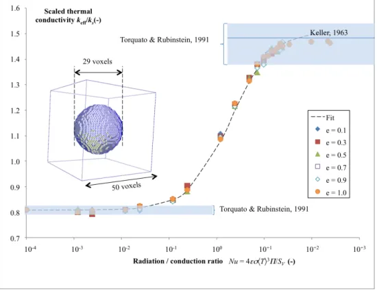
3.2. Cubic array of spherical pores with grey di↵use walls
Another test case for the method, without any infinite horizon nor flat surfaces, is the cubic array of spherical pores. A periodic cubic unit cell with 50 pixels edge size containing a single spherical cavity with a diameter of 29 pixels is used. Computations have been run using the technique based on Einstein’s formula, for various values of the emissivity and radiation/conduction ratio; the results are plotted in Figure 3.2, as scaled e↵ective conductivity ˆke↵vs. Nusselt number Nu
defined here as:
Nu = hbb⇧ ksSv
= Ps!v⇧
h| xw|i Sv (30)
All points follow the same tendency, well fitted by the following equation : ˆke↵= ˆkc,0+ ✓ ˆk 1 c,1+⇣ˆk+Nu ⌘ 1◆ 1 (31) As the importance of radiation increases, the e↵ective conductivity switches pro-gressively from a ”pure conduction value” ˆkc,0to a ”radiation-enhanced” e↵ective
conductivity that remains finite but is larger by an additive factor ˆkc,1. The inter-mediate regime involves an e↵ective conductivity of the radiating cavity ˆk+. This
behavior is straightforward to interpret, assimilating the material to the juxtaposi-tion of three blocks. The first block, with conductivity ˆkc,0, is in parallel with the
other two, themselves disposed in series, with conductivities ˆkc,1and ˆk+Nu.
The computed coefficients are compared to existing literature in Table 3.2. The value of ˆkc,0 falls within the bounds predicted by Torquato and Rubinstein
Figure 6: Scaled e↵ective conductivity of a material containing a cubic array of spherical voids with grey di↵use walls. The geometrical dimensions are given in the inset. The bounds of Torquato & Rubinstein [40] for perfectly insulating (left) and perfectly conducting spheres (right) are picted by the shaded areas; the prediction of Keller [41] for perfectly conducting spheres is de-picted by the straight line on the right.
ˆkc,0+ ˆkc,1is within the bounds given by the same authors for perfectly conducting
spheres in the same matrix, and is very close to the analytical estimate of Keller [41]. Finally, the value of ˆk+ is in reasonable agreement with the analytical result
given by Zarubin et al. [42], who obtained an e↵ective radiative conductivity for the pore only:
krad =4" Tref3 R (32)
where R = 3⇧/Svis the sphere radius. Recalling that the SMC surface
discretiza-tion method contains approximadiscretiza-tions about the sphere surface, we can conclude that the agreement with the expected values is excellent.
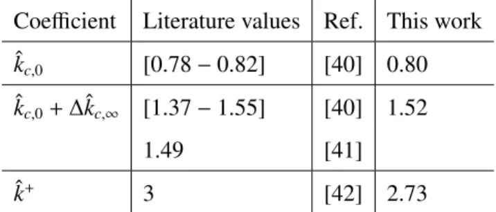
Coefficient Literature values Ref. This work
ˆkc,0 [0.78 0.82] [40] 0.80
ˆkc,0+ ˆkc,1 [1.37 1.55] [40] 1.52
1.49 [41]
ˆk+ 3 [42] 2.73
Table 1: Comparison of obtained results and estimates from literature for the e↵ective conductivity of a material containing a cubic array of spherical void with di↵use grey walls.
4. Application to a real porous medium sample
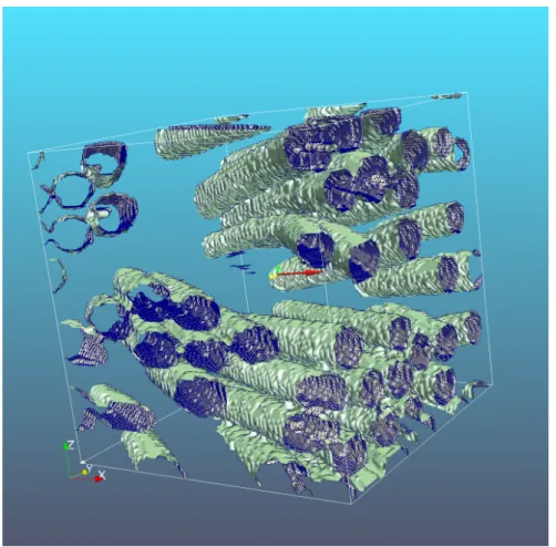
The chosen resolution domain is a 100⇥100⇥100 cubic pixels CT scan at 1.4 µm/voxel extracted from a larger data set [43]. The porosity is 67.4%, the fiber and pore diameters are respectively 10.15 and 21.16 pixels (i. e. 14.21 and 29.62 µm ). As can be seen in figure 7, the fibers are more or less parallel, but their orientation does not follow the main axes of the grid; moreover, they are not all in contact.
Computations were run in the ”average periodicity” mode, using Einstein’s relationship for the determination of the e↵ective di↵usivity. A diagonalization
Figure 7: Image used for the e↵ective conductivity computations : a portion of a CT scan of a fiber bundle.
analysis allowed retrieval of the eigenvalues and eigenvectors. By varying the emissivity and the solid-to-void transition probability, it has been checked that the e↵ective scaled conductivity eigenvalues ˆke↵,i (i = 1, 2, 3) could be cast into the
following form : ˆke↵,i= kke↵,i s = ˆkc,i+ ˆk + i (") Nu0 | {z } ˆkrad,i (33) where ˆkc,iis the conductivity obtained in purely conductive mode and in direction
i – the remaining contribution being ˆkrad,i – and the equivalent Nusselt number is
defined as [44]:
Nu0= 4 hTi3⇧
ksSv
= Ps!v⇧
"h| xw|i Sv (34)
The scaled dimensionless radiative conductivity [44] is obtained as: ˆk+ = 1 ks @ke↵ @⇣Ps!v " ⌘.Svh| xw|i ⇧ (35)
Here, @ke↵/@(Ps!v/") is, up to a constant, the slope of the conductivity vs. Tref3
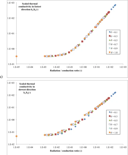
curve. Figure 8 illustrates the verification of eq. (33) for the fastest and slowest directions of heat transfer. As could be expected, the pure conduction value in the fastest direction is slightly lower than (1 ⇧), which is the law-of-mixtures prediction. Somewhat more surprisingly, there is also a non-zero value – though small – in the slowest direction of transfer. This arises from the chosen boundary conditions, which connect together apparently unconnected fibers. Moreover, the law of mixtures is less well respected for high emissivities, as could be expected since the fibers and voids are not in a parallel arrangement.
Figure 9 displays the evolution of the angle between the fastest transfer direc-tion (red arrow on fig. 10) and the z axis (almost vertical on the images), as a function of the radiation /conduction ratio Nu0. A clear change occurs between
Nu0 =10 2and 1, in coincidence with the curvature change of the log-log curves
of figure 8. This Nu0range ofh10 2; 1iclearly defines what can be called a
a)
b)
Figure 8: Scaled e↵ective conductivities of a fibrous image sample in the fastest(a) and slowest (b) directions, as a function of the radiation/di↵usion ratio Nu0, for various values of the emissivity ".
Figure 9: Evolution of the angle between the fastest di↵usion direction (red arrow on fig 10) and the z direction (green axis on fig. 10), as a function of the equivalent Nusselt number.
In figure 10, we can see the orientation of the eigenvectors obtained in purely conductive mode and in radiation-dominated mode (Ps!v=0.5 and " = 0.1, lead-ing to Nu0=130, i.e. after the transition regime). The direction of fastest di↵usion
follows very well the fiber direction in pure conduction mode, as expected. On the other hand, when radiation is not negligible, transfer becomes important in the transverse directions (eigenvalues are approximately 1/3 of the fastest direction), and the eigenvector set is rotated downwards.
The ˆk+ values are plotted as a function of " in fig. 11, showing a weak
de-pendence. The absolute values are small as compared to what Bellet et al. [44] and Taine et al. [45] give for periodic arrays of parallel bundles. This is not a surprising fact, because there is a very important di↵erence between this image and ideal arrays : there is no infinite horizon here. On the other hand, the values determined by Chahlafi et al. [46] in non-ideal images of bundles of damaged rods are in good agreement with ours. Nonetheless, the evolution of ˆk+ with " is
very similar to the ideal case, i.e. a very weak dependency.
It should be noted that these results on e↵ective conductivities are subjected to a validity criterion, as discussed thoroughly by Gomart & Taine [47], namely :
hrTi
Tref << e↵ (36)
where e↵is an e↵ective absorption coefficient, roughly of the order of magnitude
of the internal surface area. 5. Conclusion
This paper has presented the principles and implementation of a mixed random-walk algorithm designed for the resolution of the coupled radiative-conductive heat transfer in a porous medium with an opaque and a transparent phase (void pores). The algorithm has been used for the determination of e↵ective conductiv-ities in porous media whereby conduction in the solid and radiation on the voids
a) b)
c) d)
Figure 10: Heat transfer eigenvectors in a fibrous bundle CT image. a,b): pure conduction, c,d) : with radiation. The eigenvectors colors are red, green, yellow in decreasing order of magnitude, and are displayed in the center of the image (green and yellow are hardly visible on top). A sample radiative/conductive trajectory portion is rendered as white lines in the bottom images.
Figure 11: Evolution of the dimensionless radiative conductivity as a function of the emissivity. The dotted lines refer to the values determined by Chahlafi et al. [46]
are coupled, in the limit of small temperature perturbations, as compared to the average medium temperature. Validation with respect to analytical cases has been obtained; an example of application to actual porous media has shown the poten-tiality of the computational tool, by showing how the e↵ective conduction tensor changes when switching from purely conductive to mixed conductive/radiative transfer. Further work has to be carried out in several directions. First, a very severe limitation in the use of the presented method arises from the linearisation hypothesis : only very small temperature gradients are admissible, following the Gomart-Taine criterion. The determination of e↵ective conductivities could be extended to the case of high gradients, by removing the linearisation hypothesis. In numerical practice, this would require to design an iterative numerical scheme in which the transition probability Ps!vwould be recomputed as a function of the local temperature and the random walks launched again, until convergence. Ap-plication of the model to situations where the boundaries have an influence on the overall conductivity can also be treated with the provided flux/gradient method.
The algorithm could be also used for the determination of e↵ective optical properties, or for direct simulations of a flash experiment. Many enrichments of the modeled physics - considering grey media, for instance - may be attempted too. Moreover, application to other types of porous media than those discussed here would be of great interest.
Acknowledgements
The author wishes to acknowledge Pr. Jean Taine (EM2C, ECP, Paris), Pr. Al-berto Ortona (ICIMSI, Lugano, Switzerland), Dr. Benoˆıt Rousseau (LTN, CNRS, Nantes), and Dr. Cyril Caliot (PROMES, CNRS, Perpignan) for fruitful discus-sions, and two anonymous reviewers for suggesting many improvements.
Symbol Meaning Unit
a Thermal di↵usivity m2.s 1
cp Heat capacity per unit mass J.kg 1.K 1
hbb Radiative heat transfer coefficient W.m 2.K 1
I Radiative intensity W.m 4
Itot Total radiative intensity W.m 4
I Equilibrium black body radiative intensity W.m 4
k Thermal conductivity W.m 1.K 1
ˆk Scaled thermal conductivity
-Lx, y or z Cell dimensions m
Lpix Pixel size m
n Exterior normal to a surface element
-N Number of walkers
-Nu Nusselt number
-Pv!v Probability to be reflected in void
-Ps!v Probability to be transferred from solid to void
-q Heat flux W.m 2
R Sphere radius m
S Surface m2
Sv Surface area per unit volume m 1
T Temperature K
ˆT Temperature perturbation K
t Time s
Symbol Meaning Unit
↵ Wall absorptivity
-Random Gaussian number
-x Position increment m
t Time increment s
H Enthalpy excess per walker J
q Flux element W.m 2
S Surface element m2
V Volume element m3
" Wall emissivity
-✓ Polar angle rad
Volume absorption coefficient m 1
⇧ Porosity
-⇢ Density kg.m 3
Stefan’s constant W.m 2.K 4
Azimuthal angle rad
Symbol Meaning Unit
h•i Average
h•inx Face-average
h•is Solid-phase intrinsic average
˜• Perturbation •in incident •e emitted •e↵ e↵ective •max maximal •ref reference •rad radiative
•s relative to the solid phase
•+ radiation-related
References
[1] S. Heng, A. J. Sherman, Advanced materials for thermal protection system, in: Space technology and applications international forum - 1st conference on commercial development of space; 1st conference on next generation launch systems; 2nd spacecraft thermal control symposium; 13th sympo-sium on space nuclear power and propulsion, Vol. 361 of AIP Conf. Procs, Albuquerque, New Mexico (USA), 1996, pp. 635–638.
[2] E. Venkatapathy, B. Laub, G. Hartman, J. Arnold, M. Wright, G. A. Jr., Thermal protection system development, testing, and qualification for atmo-spheric probes and sample return missions: Examples for Saturn, Titan and Stardust-type sample return, Advances in Space Research 44 (1) (2009) 138 – 150. doi:10.1016/j.asr.2008.12.023.
[3] D. Barlev, R. Vidu, P. Stroeve, Innovation in concentrated solar power, Solar Energy Materials and Solar Cells 95 (10) (2011) 2703–2725.
[4] C. C. Agrafiotis, I. Mavroidis, A. G. Konstandopoulos, B. Ho↵schmidt, P. Stobbe, M. Romero, V. Fernandez-Quero, Evaluation of porous silicon carbide monolithic honeycombs as volumetric receivers/collectors of con-centrated solar radiation, Solar Energy Materials and Solar Cells 91 (6) (2007) 474 – 488. doi:10.1016/j.solmat.2006.10.021.
[5] H. K. Tran, C. E. Johnson, D. J. Rasky, F. C. L. Hui, M.-T. Hsu, T. Chen, Y. K. Chen, D. Paragas, L. Kobayashi, Phenolic impregnated carbon abla-tors (pica) as thermal protection systems for discovry missions, Technical Memorandum 110440, NASA, ARC, Mo↵ett Field, CA (1997).
[6] M. F. Modest, Radiative Heat Transfer, 3rd Edition, Academic Press, New York, S. Francisco, 2013.
[7] R. Singh, H. Kasana, Computational aspects of e↵ective thermal conduc-tivity of highly porous metal foams, Applied Thermal Engineering 24 (13) (2004) 1841 – 1849. .
[8] V. V. Calmidi, R. L. Mahajan, The e↵ective thermal conductivity of high porosity fibrous metal foams, J. Heat Transfer 121 (2) (1999) 466–471. [9] J. Truelove, Three-dimensional radiation in absorbing-emitting-scattering
media using the discrete-ordinate approximation, J. Quant. Spectrosc. & Rad. Transf. 39 (1988) 27–31.
[10] L. Zhang, J.-M. Zhao, L.-H. Liu, Finite element method for modelling radia-tive transfer in semitransparent graded index cylindrical medium, J. Quant. Spectrosc. & Rad. Transf. 110 (2009) 1085–1096.
[11] T. Fiedler, I. Belova, A. Ochsner, G. Murch, Non-linear calculations of tran-sient thermal conduction in composite materials, Computational Materials Science 45 (2009) 434–438.
[12] A. Milandri, F. Asllanaj, G. Jeandel, J. R. Roche, Heat transfer by radiation and conduction in fibrous media without axial symmetry, J. Quant. Spec-trosc. & Rad. Transf. 74 (5) (2002) 585–603.
[13] C. Berthon, P. Charrier, B. Dubroca, An asymptotic preserving relaxation scheme for a moment model of radiative transfer, C. R. Acad. Sci. Math. 344 (7) (2007) 467–472.
[14] H. Hottel, E. Cohen, Radiant heat exchange in a gas-filled enclosure: Al-lowance for nonuniformity of gas temperature, AIChE J. 4 (1958) 3–14. [15] B. Zeghondy, J. Taine, Determination of anisotropic absorption and
extinc-tion coefficients of a tomographed real porous medium, in: Proc. ASME Intl. Mech. Engng Congress, Anaheim, CA, Vol. 3 of ASME Procs Heat Transfer, ASME, ASME, Anaheim, Ca, 2004, pp. 291–296.
[16] B. Zeghondy, E. Iacona, J. Taine, Determination of the anisotropic radiative properties of a porous material by radiative distribution function identifica-tion (rdfi), Internaidentifica-tional Journal of Heat and Mass Transfer 49 (19-20) (2006) 3702–3707.
[17] M. Tancrez, J. Taine, Direct identification of absorption and scattering coef-ficients and phase function of a porous medium by a Monte Carlo technique, International Journal of Heat and Mass Transfer 47 (2) (2004) 373–383. [18] B. Rousseau, D. de Sousa Meneses, P. Echegut, M. D. Michiel, J.-F. Thovert,
Prediction of thermal radiative properties of an X-ray µ-tomographied porous silica glass, Applied Optics 46 (20) (2007) 4266–4276.
[19] M. Loretz, R. Coquard, D. Baillis, E. Maire, Metallic foams : Radiative properties/comparison between di↵erent models, J. Quant. Spectrosc. & Rad. Transf. 109 (2008) 16–27.
[20] M. Loretz, E. Maire, D. Baillis, Analytical modelling of the radiative prop-erties of metallic foams: Contribution of X-ray tomography, Advanced En-gineering Materials 10 (4) (2008) 352–360.
[21] S. Volz, Monte carlo method, in: S. Volz (Ed.), Microscale and Nanoscale Heat Transfer, 1st Edition, Vol. 107 of Topics Appl. Physics, Springer-Verlag, Berlin Heidelberg, 2007, Ch. 7, pp. 133–154.
[22] J. R. Howell, M. Perlmutter, The calculation of nonlinear radiation transport by a Monte Carlo method: Statistical physics, Methods in Computational Physics 1 (1961) 43–65.
[23] J.-F. Luo, H.-L. Yi, B. Zhen, H.-P. Tan, Solution to coupled heat transfer in a rectangular medium with black surfaces with ray tracing method, Kung Cheng Je Wu Li Hsueh Pao/Journal of Engineering Thermophysics 31 (1) (2010) 90–93.
[24] P. Vueghs, H. P. de Koning, O. Pin, P. Beckers, Use of geometry in finite el-ement thermal radiation combined with ray tracing, J. Comput. Appl. Math. 234 (7) (2010) 2319–2326. doi:10.1016/j.cam.2009.08.088.
[25] D. Terris, K. Joulain, D. Lemonnier, D. Lacroix, P. Chantrenne, Prediction of the thermal conductivity anisotropy of si nanofilms. Results of several nu-merical methods, International Journal of Thermal Sciences 48 (2009) 1467– 1476.
random walk algorithms for fiber-scale modeling of chemical vapor in-filtration, Computational Materials Science 50 (3) (2011) 1157 – 1168. doi:10.1016/j.commatsci.2010.11.015.
[27] G. L. Vignoles, Modelling binary, Knudsen and transition regime di↵usion inside complex porous media, J. de Phys. IV 5 (C5) (1995) 159–166. [28] S. Chandrasekhar, Stochastic problems in physics and astronomy, Rev. Mod.
Phys. 15 (1) (1943) 1 – 89.
[29] I.-C. Kim, S. Torquato, E↵ective conductivity of suspensions of hard spheres by Brownian motion simulation, J. Appl. Phys. 69 (4) (1991) 2280–2289. [30] G. L. Vignoles, W. Ros, I. Szelengowicz, C. Germain, A Brownian motion
algorithm for tow scale modeling of chemical vapor infiltration, Comput. Mater. Sci. 50 (6) (2011) 1871–1878. doi:10.1016/j.commatsci.2011.01.031. [31] O. Almanza, M. R. P´erez, J. D. Saja, Prediction of the radiation term in the thermal conductivity of crosslinked closed cell polyolefin foams, Journal of Polymer Science Part B : Polymer Physics 38 (2000) 993–1004.
[32] C. D. Micco, C. Aldao, Radiation contribution to the thermal conductivity of plastic foams, Journal of Polymer Science Part B : Polymer Physics 43 (2005) 190–192.
[33] S. Delettrez, Elaboration par voie gazeuse et caract´erisation de c´eramiques alv´eolaires base pyrocarbone ou carbure de silicium, Ph.D. thesis, University Bordeaux I (2008).
[34] W. Kinzelbach, G. Uffink, The random walk method and extensions in groundwater modelling, in: Transport Processes in Porous Media, Springer, 1991, pp. 761–787.
[35] E. M. LaBolle, G. E. Fogg, A. F. B. Thompson, Random-walk simulation of transport in heterogeneous porous media : Local mass-conservation problem and implementation methods, Water Resources Research 32 (3) (1996) 583– 593.
[36] G. L. Vignoles, M. Donias, C. Mulat, C. Germain, J.-F. Delesse, Simplified marching cubes: An efficient discretization scheme for simulations of depo-sition/ablation in complex media, Computational Materials Science 50 (3) (2011) 893 – 902. doi:10.1016/j.commatsci.2010.10.027.
[37] A. Einstein, Investigations on the theory of the brownian movement (Trans-lated by A. D. Cowper), Dover Edition, Berlin, 1956.
[38] F. Transvalidou, S. V. Sotirchos, E↵ective di↵usion coefficient in square ar-rays of filament bundles, AIChE J. 42 (9) (1996) 2426–2438.
[39] F. M¨uller-Plathe, Cause and e↵ect reversed in non-equilibrium molec-ular dynamics: an easy route to transport coefficients, Computa-tional and Theoretical Polymer Science 9 (3-4) (1999) 203 – 209. doi:http://dx.doi.org/10.1016/S1089-3156(99)00006-9.
[40] S. Torquato, J. Rubinstein, Improved bounds on the e↵ective conductivity of high contrast suspensions, Journal of Applied Physics 69 (10) (1991) 7118– 7125. doi:10.1063/1.347600.
[41] J. B. Keller, Conductivity of a medium containing a dense array of perfectly conducting spheres or cylinders or nonconducting cylinders, Journal of Ap-plied Physics 34 (4) (1963) 991–993. doi:10.1063/1.1729580.
[42] V. Zarubin, G. Kuvyrkin, I. Savelyeva, Radiative-conductive heat trans-fer in a spherical cavity, High Temperature 53 (2) (2015) 234–239. doi:10.1134/S0018151X15020248.
[43] O. Coindreau, G. L. Vignoles, Assessment of geometrical and transport properties of a fibrous C/C composite preform as digitized by X-ray com-puted micro-tomography. Part I : Image acquisition and geometrical proper-ties, J. Mater. Res. 20 (9) (2005) 2328–2339.
[44] F. Bellet, E. Chalopin, F. Fichot, E. Iacona, J. Taine, RDFI determination of anisotropic and scattering dependent radiative conductivity tensors in porous media: Application to rod bundles, International Journal of Heat and Mass Transfer 52 (5-6) (2009) 1544–1551.
[45] J. Taine, F. Bellet, V. Leroy, E. Iacona, Generalized radiative transfer equa-tion for porous medium upscaling: Applicaequa-tion to the radiative Fourier laws, International Journal of Heat and Mass Transfer 53 (19-20) (2010) 4071– 4081.
[46] M. Chahlafi, F. Bellet, F. Fichot, J. Taine, Radiative transfer within non Bee-rian porous media with semitransparent and opaque phases in non equilib-rium: Application to reflooding of a nuclear reactor., International Journal of Heat and Mass Transfer 55 (13-14) (2012) 3666–3676.
[47] H. Gomart, J. Taine, Validity criterion of the radiative fourier law for an absorbing and scattering medium, Physical Review E - Statistical, Nonlinear, and Soft Matter Physics 83 (2) (2011) 021202.
Appendix A. Evaluation of the average last step size before collision at the interface
The average last step size h| xw|i may be computed assuming that the walker
lies at a point M distant from the surface by length h; the step size xdis such that
its variance isD x2 d
E
=6a t and obeys a Maxwellian distribution: p ( xd) d3x = 1 8 (⇡a t)32 exp x2+y2+z2 4a t ! dxdydz (A.1)
The mean step size is h| xd|i =
q
16a t
⇡ . The length of the last step is simply
obtained by setting y = h in the modulus of xd:
| xw| =
p
x2+h2+z2 (A.2)
Let us assume r2=x2+z2. We have to consider all events where the wall is hit or
trespassed, so that the probability density has to be: Ph=P walker hits the wall distant by h =
Z 1 r=0
Z 1
y=hp ( xd) 2⇡rdrdy (A.3)
Numerically, one has:
Ph= 1 2erfc h 2pa t ! (A.4) The probability density is therefore :
p(h)dh = r ⇡ 4a terfc h 2pa t ! dh (A.5)
The average over all possible values of h of the last step size is given by : h| xw|i = Z 1 h=0 "Z 1 r=0| xw| p(r)dr # p(h)dh (A.6)
or, expanding the expression: h| xw|i = p ⇡ 8 (a t)32 Z 1 h=0 "Z 1 r=0 p r2+h2exp r2 4a t ! d(r2)#erfc h 2pa t ! dh (A.7)
Evaluating the integral between brackets gives: h| xw|i = Z 1 h=0 " p⇡ 2pa th + ⇡ 2exp h2 4a t ! erfc h 2pa t !# erfc h 2pa t ! dh (A.8) The two integrals appearing in this expression are evaluated separately. The first one is: I1= Z 1 h=0 h p⇡ 2pa terfc h 2pa t ! dh = p ⇡a t 2 (A.9)
The second one may be evaluated numerically: I2= Z 1 h=0 ⇡ 2erfc h 2pa t !2 exp h2 4a t ! dh ⇡ 0.8687pa t (A.10)
Summing both, we get :
h| xw|i ⇡ 1.75496
p
a t (A.11)
Comparing to the average step size and to the root mean square step size, we finally get: h| xw|i ⇡ 0.777645 h| xd|i (A.12) and: h| xw|i ⇡ 0.716459 qD x2 d E (A.13) Appendix B. Treatment of the zero-thickness slabs
Fig B.12 is an example of a zero-thickness slab that may result from the SMC discretization scheme. For the walk algorithm, one defines a probability of not traversing such a surface as:
Prefl= 1 X n=1 "Ps!v(1 Ps!v)2n = 2 P" s!v (B.1)
Then, depending on whether a random number with uniform density on the unit interval is smaller or larger than this probability, the walker is reflected by or transmitted through the slab, respectively.