HAL Id: hal-01579523
https://hal.inria.fr/hal-01579523
Submitted on 31 Aug 2017
HAL is a multi-disciplinary open access
archive for the deposit and dissemination of
sci-entific research documents, whether they are
pub-lished or not. The documents may come from
teaching and research institutions in France or
abroad, or from public or private research centers.
L’archive ouverte pluridisciplinaire HAL, est
destinée au dépôt et à la diffusion de documents
scientifiques de niveau recherche, publiés ou non,
émanant des établissements d’enseignement et de
recherche français ou étrangers, des laboratoires
publics ou privés.
Morphorider: Acquisition and Reconstruction of 3D
Curves with Mobile Sensors
Tibor Stanko, Nathalie Saguin-Sprynski, Laurent Jouanet, Stefanie Hahmann,
Georges-Pierre Bonneau
To cite this version:
Tibor Stanko, Nathalie Saguin-Sprynski, Laurent Jouanet, Stefanie Hahmann, Georges-Pierre
Bon-neau. Morphorider: Acquisition and Reconstruction of 3D Curves with Mobile Sensors. IEEE Sensors
2017, Oct 2017, Glasgow, United Kingdom. pp.1-3, �10.1109/ICSENS.2017.8234266�. �hal-01579523�
Morphorider:
Acquisition and Reconstruction of 3D Curves with Mobile Sensors
Tibor Stanko
1,2, Nathalie Saguin-Sprynski
1, Laurent Jouanet
1, Stefanie Hahmann
2, and Georges-Pierre Bonneau
2 1CEA, LETI, MINATEC Campus, Universit´e Grenoble Alpes
2
Universit´e Grenoble Alpes, CNRS (Laboratoire Jean Kuntzmann), INRIA
firstname.lastname@
{cea,inria}.fr
Abstract—This paper introduces a new method for real-time shape sensing. Using a single inertial measurement unit (IMU), our method enables to scan physical objects and to reconstruct digital 3D models. By moving the IMU along the surface, a network of local orientation data is acquired together with traveled distances and network topology. We then reconstruct a consistent network of curves and fit these curves by a globally smooth surface. To demonstrate the feasibility of our approach, we have constructed a mobile device called the Morphorider, which is equipped with a 3A3M-sensor node and an odometer for distance tracking.
Index Terms—Shape measurement, sensor systems, reconstruc-tion algorithms.
I. INTRODUCTION& RELATEDWORK
The use of inertial micro sensors is common in many domains. Traditionally, they are at the heart of navigation systems to maneuver aircrafts, satellites or unmanned vehicles. Only recently, the use of inertial sensors for curve and surface reconstruction has emerged. The novelty of this reconstruction problem is to deal purely with orientation and distance data instead of point clouds traditionally acquired using optical 3D scanners. While a few pioneering methods were proposed in the last decade, shape sensing still remains a challenging task due to the inherent issues: inertial sensors only provide local orientations but no spatial locations; moreover, raw data from inertial sensors are inconsistent and noisy.
Previous works on shape from sensors proposed devices with a fixed connectivity and known distances between sensor nodes: the sensors were organized uniformly on a 1D ribbon [1] or on a regular 2D grid [2,3]. Multiple ribbons were employed to acquire networks of curves on a surface, using a comb structure [4] or patches with boundary from geodesic curves [5]. However, these ribbons cannot be placed on the surface arbitrarily as they will inevitably follow geodesic curves. Grids of sensor nodes are limited to specific types of surfaces (e.g. developable surfaces isometric to planar sheets). While most existing methods work in real-time, they adopt various heuristics to glue the acquired curves together in order to have a closed network with proper topology of ribbons or a grid.
This paper considers a different setup: a device with a single IMU is moved along a virtual network of curves on the scanned surface, and the data is acquired interactively. The advantages are multiple. a) The topology of the curve network
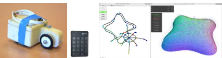
Fig. 1. Left: the Morphorider and the wireless keypad used for marking nodes during acquisition. Right: screenshots of our acquisition and reconstruction applications.
is no longer fixed by the device. Consequently, this allows us to acquire a much broader family of shapes than with previous methods. b) The size of the object is no longer limited by the size of a pre-designed grid. c) A very dense set of orientation data is available, which significantly improves the precision of our method.
Our contribution is twofold. First, we introduce the
Mor-phorider, a prototype of a sensor-instrumented device for dy-namic acquisition of orientations and distances along surface curves. Second, we demonstrate how the inherent noise and inconsistency of the data captured by the sensor device can be handled to produce a network of smooth curves on the scanned surface. Our main insight is to perform the filtering in the space of orientations and only integrate afterwards to get the positions. We apply the framework introduced in [6] in order to integrate the orientation data. Note that the proposed framework is not limited to the dynamic setup, and can also be used in combination with fixed-topology devices without modification. Possible applications are countless and include smart materials [5], shape digitization [6], medical scanning [3] and Structural Health Monitoring (SHM) [2].
II. ACQUISITION DEVICE
In this section we describe the Morphorider, a novel MEMS-based dynamic device, which is used for data acquisition. The key idea is to provide a device which can trace an uncon-strained virtual network of curves on the scanned surface. This enables acquisition and reconstruction of a broader family of shapes than existing fixed-topology devices.
a) Sensors of orientation: To measure the orientation of the device, we use inertial sensors able to provide their rotation with respect to a measured field. Concretely, we use: a 3-axis accelerometer providing the angle with respect to the Earth’s
gravity field when static (the vertical direction); and a 3-axis magnetometer providing the angle with respect to the Earth’s magnetic field, as long as there are no magnetic perturbations. An orthonormal frame that represents the 3D orientation is determined by combining the information from both sensors. The sensors are placed in the device so that one of the axes of the orthonormal frame is aligned with the motion axis. The orientations are estimated from sensor measurements by solving the Wahba’s problem using SVD [7,8].
b) Sensor of displacement: Orientations are by them-selves not sufficient to reconstruct the spatial locations, we also need to know the displacement of the device along the scanned curves. To this end, we use an odometer: the encoder disk sends a tick when 1/500 of a round is traveled. The displacement of the Morphorider has to be controlled to avoid slidings.
c) Data collection: The sensor data are read via a serial bus connected to a microcontroller managed by a software driver allowing to communicate with the device. Values from odometer and inertial sensors are read sequentially. The ac-quisition is wireless: Morphorider is equipped with a battery and the communication with the host computer is done using a Bluetooth connection.
d) Acquisition process: We use a MATLAB interface to acquire data. In addition to measuring the orientations and distances along curves, we also specify the network topology: prior to acquisition, we assign a unique index between0 and n − 1 to each of the n network nodes (intersections). The acquisition is controlled remotely using a wireless numpad (Fig. 1 left). When starting a new curve, we first indicate if the curve is at the boundary or in the interior. Then, every time the device passes through a node, we record its index.
III. RECONSTRUCTION OF CURVE NETWORK The Morphorider provides orientations and distances along a network of smooth curves on a surface. We will now use these data to reconstruct the network: this network is then interpolated with existing surfacing methods.
a) Problem formulation: We consider a collectionΓ of G1
smooth curves embedded on a 2-manifold surfaceS ⊂ R3
. Denote by x : [0, L] → R3
the natural parametrization of γ ∈ Γ where L is the length of γ. For a fixed point x on the curve, the orthonormal Darboux frame D = (T, B, N) consists of the unit tangent vector T= ˙x, the outward surface normal N, and the binormal B = N × T [9]. We represent the Darboux frame D as an orientation matrix A = [T B N] which is a member of the special orthogonal group SO(3).
Knowing the topology of network and a set of orientations Ai = A (x (di)) sampled at known distances di ∈ [0, L] for
each curveγ, the goal is to retrieve the unknown positions x.
b) Pre-filtering: The noisy raw data are first pre-processed to obtain a uniform sampling with respect to arc length. In this step, we use unit quaternions to represent the orientations; see [7] for details and conversion relations. First, we remove the outliers and the duplicate measures; we then fix the sampling distance hfix and compute uniform
distance parameterstk= kh for each curve γ with length L,
whereh = L/N and N = round(L/hfix). The corresponding
unit quaternionq¯k is computed by convoluting the measured
orientations with a Gaussian kernel: ¯
qk = meanqi∈γwk,iqi, wk,i= exp
[ −1 2 ( tk− di σhfix )2] . The parameter σ ∈ [0.2, 0.5] controls the radius of convolu-tion. Means are computed using the q method [7].
c) Filtering by regression on SO(3): The next step is to smooth the orientations and ensure the consistency of surface normals at intersections of curves. To this end we use a variant of smoothing splines on the manifold SO(3). Recall that a
smoothing spline x: [t0, tN] → Rnfor a set of points pi ∈ Rn
minimizes the energy
N ∑ i=0 ∥x(ti) − pi∥ 2 + ∫ tN t0 λ∥ ˙x∥2 + µ∥¨x∥2 dt. (1) The weights λ, µ > 0 control stretching and bending of the spline, respectively. We will write this energy as E = E0+
λE1+µE2. Similarly, smoothing splines have been defined for
data on Riemannian manifolds [10]. To smooth the orientation data Ai on the manifold SO(3), we use the following energies
(see [11] for details): E0(γ) = N ∑ i=0 ∥Xi− Ai∥ 2 F, E1(γ) = 1 h N −1 ∑ i=0 ∥Xi− Xi+1∥ 2 F, E2(γ) = 1 h3 N −1 ∑ i=1
skew(X⊤i (Xi+1+ Xi−1)
)
2
F. (2)
In our setup, the raw data Ai is associated to a network
Γ and the above energy terms are summed over all curves γ ∈ Γ. Simultaneously with regression on SO(3), we solve the consistency constraints as follows. Let Xi, ˜Xj be the
local Darboux frames of two curves at their intersection. Then the two frames are called consistent if Xi is obtained by
rotating ˜Xj around the surface normal. Denote byN the set
of all such pairs (Xi, ˜Xj
)
. To enforce consistency, we add a term penalizing the difference in projection on the normal component EN(Γ) = ∑ (Xi, ˜Xj)∈N Xi|N− ˜Xj|N 2 . (3)
The final energy is minimized using Riemannian trust region algorithm [12].
d) Integration: The positions x are computed by solving Poisson’s equation ∆ x = ∇ · T where T is the tangent field extracted from the filtered orientations X. The differ-ential operators are discretized via finite differences: ∆ xi =
1
h2(xi−1− 2xi+ xi+1) , ∇ Ti= h1(Ti− Ti−1). The above
discretization is valid for all interior vertices. At endpoints of open curves, we directly impose the boundary conditions
1
h(x1− x0) = T0, 1
h(xN − xN −1) = TN. The resulting
linear system LX = T is sparse with at most three non-zero coefficients per row.
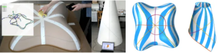
Fig. 2. Left: acquisition of the two fabricated shapes used for evaluation. Right: reconstructed networks surfaced using the method of [13].
h= 6.40% h= 3.20% h= 1.60% h= 0.80% h= 0.40% 0% 2%
0% 4%
Fig. 3. Reconstruction error for decreasing edge length h. For filtering, we used the weights λ = µ = 1. All lengths are relative to the diameter (AABB diagonal) of corresponding ground truth surface.
e) Surfacing: The reconstructed curve network is sur-faced using one of the existing methods that take into account the available surface normals along the curves [6].
IV. EVALUATION& CONCLUSIONS
To enable a thorough evaluation and comparison with respect to known data, we used the Morphorider to acquire curves on two physical objects fabricated from digital models (Fig. 2): the LILIUM (1.00m×1.00m×0.25m) and the CONE (1.00m×1.00m×2.00m). We then computed reconstruction error for the acquired networks: for each point x in the reconstructed network, the error is defined as the distance between x and its closest point xS on the ground truth
surface. The results for decreasing edge length h are shown in Fig. 3 and in Table I. The choice of h for concrete applications depends on the required precision or computation time (Table I).
The presented Morphorider is an innovative device provid-ing a new way to scan physical shapes. By its displacement on the surface, our approach provides a robust curve network ready for surfacing (Fig. 2). Limitations of our method are device-related: size of the device may prevent acquisition of high-curvature regions and small details. The next generation prototype is in development.
REFERENCES
[1] N. Sprynski, D. David, B. Lacolle, and L. Biard. “Curve Reconstruction via a Ribbon of Sensors”. In: Proc. 14th
Int. Conf. Electronics Circuits Systems (ICECS). 2007, pp. 407–410.
[2] N. Saguin-Sprynski, L. Jouanet, B. Lacolle, and L. Biard. “Surfaces Reconstruction Via Inertial Sensors for Monitoring”. In: EWSHM. 2014.
TABLE I
RECONSTRUCTION ERROR FOR DECREASING EDGE LENGTHh. ALL LENGTHS ARE RELATIVE TO THE DIAMETER(AABBDIAGONAL)OF THE
CORRESPONDING GROUND TRUTH SURFACE.
6.4% 3.2% 1.6% 0.8% 0.4% 0% 1% 2% 3% h e rr or max error (%) * LILIUM 3.15 2.68 2.46 2.38 2.35 * CONE 1.59 1.15 1.17 1.13 1.21 mean error (%) • LILIUM 1.36 1.23 1.19 1.17 1.15 • CONE 0.61 0.49 0.46 0.45 0.45 reconstruction time (ms) • CONE 184 339 654 1319 3705 • LILIUM 55 122 247 478 973
[3] A. Hermanis, R. Cacurs, and M. Greitans. “Acceleration and Magnetic Sensor Network for Shape Sensing”. In:
IEEE Sensors J.16.5 (Mar. 2016), pp. 1271–1280. [4] N. Sprynski, B. Lacolle, and L. Biard. “Motion Capture
of an Animated Surface via Sensors’ Ribbons”. In:
Int. Conf. Pervasive and Embedded Computing and Communication Systems (PECCS). 2011, pp. 421–426. [5] M. Huard, N. Sprynski, N. Szafran, and L. Biard. “Re-construction of quasi developable surfaces from ribbon curves”. In: Num. Alg. 63.3 (2013), pp. 483–506. [6] T. Stanko, S. Hahmann, G.-P. Bonneau, and N.
Saguin-Sprynski. “Shape from sensors: Curve networks on sur-faces from 3D orientations”. In: Comput Graph (Proc.
SMI)(2017).
[7] J. L. Crassidis, F. L. Markley, and Y. Cheng. “Survey of nonlinear attitude estimation methods”. In: J. Guid.
Control Dyn.30.1 (2007), pp. 12–28.
[8] S. Bonnet et al. “Calibration methods for inertial and magnetic sensors”. In: Sensors and Actuators A:
Phys-ical156.2 (2009), pp. 302–311.
[9] M. P. do Carmo. Differential Geometry of Curves and
Surfaces. Pearson, 1976.
[10] N. Boumal and P.-A. Absil. “A discrete regression method on manifolds and its application to data on SO(n)”. In: Proc. 18th IFAC WC. 2011, pp. 2284–2289. [11] N. Boumal. “Interpolation and Regression of Rotation
Matrices”. In: Geom.Sci.Inf. 2013, pp. 345–352. [12] W. Huang, P.-A. Absil, K. A. Gallivan, and P. Hand.
ROPTLIB: An object-orient. C++ lib. for optim. on Riemannian manifolds. Tech. rep. FSU16-14.v2. 2016. [13] T. Stanko, S. Hahmann, G.-P. Bonneau, and N.
Saguin-Sprynski. “Surfacing curve networks with normal con-trol”. In: Comput Graph 60 (Nov. 2016), pp. 1–8.