Complexity leads to randomness in chaotic systems

(1)

HAL Id: hal-00627604

https://hal.archives-ouvertes.fr/hal-00627604

Submitted on 29 Sep 2011

HAL is a multi-disciplinary open access

archive for the deposit and dissemination of

sci-entific research documents, whether they are

pub-lished or not. The documents may come from

teaching and research institutions in France or

L’archive ouverte pluridisciplinaire HAL, est

destinée au dépôt et à la diffusion de documents

scientifiques de niveau recherche, publiés ou non,

émanant des établissements d’enseignement et de

recherche français ou étrangers, des laboratoires

René Lozi

To cite this version:

René Lozi. Complexity leads to randomness in chaotic systems. A.H. Siddiqi, R.C. Singh, P.

Man-chanda. Mathematics in Science and Technology: Mathematical Methods, Models and Algorithms in

Science and Technology. Proceedings of the Satellite Conference of ICM, 15-17 August 2010 Delhi,

India, World Scientific, pp.93-125, 2011. �hal-00627604�

(2)

Singapore (2011) pp. 93-125.

COMPLEXITY LEADS TO RANDOMNESS IN CHAOTIC

SYSTEMS

RENÉ LOZI

Laboratory J. A. Dieudonné, UMR CNRS 6621, University of Nice Sophia-Antipolis, Parc Valrose, 06108 Nice Cedex 02, France

and

Institut Universitaire de Formation des Maîtres Célestin Freinet-académie de Nice, University of Nice-Sophia-Antipolis, 89 avenue George V, 06046 Nice Cedex 1, France

Abstract— Complexity of a particular coordinated system is the degree of difficulty in

predicting the properties of the system if the properties of the system's correlated parts are given. The coordinated system manifests properties not carried by individual parts. The subject system can be said to emerge without any “guiding hand”. In systems theory and science, emergence is the way complex systems and patterns arise out of a multiplicity of relatively simple interactions. Emergence is central to the theories of integrative levels and of complex systems. The emergent property of the ultra weak multidimensional coupling of

p 1-dimensional dynamical chaotic systems for which complexity leads from chaos to

randomness has been recently pointed out.

Pseudorandom or chaotic numbers are nowadays used in many areas of contemporary technology such as modern communication systems and engineering applications. Efficient Chaotic Pseudo Random Number Generators (CPRNG) have been recently introduced. They use the ultra weak multidimensional coupling of p 1-dimensional dynamical systems which preserves the chaotic properties of the continuous models in numerical experiments. Together with chaotic sampling and mixing processes, the complexity of ultra weak coupling leads to families of CPRNG which are noteworthy. In this paper we improve again these families using a double threshold chaotic sampling instead of a single one. A window of emergence of randomness for some parameter value is numerically displayed. Moreover we emphasize that a determining property of such improved CPRNG is the high number of parameters used and the high sensitivity to the parameters value which allows choosing it as cipher-keys.

1. Introduction

Characterizing complexity is not easy and there are in science a number of approaches to do it. Many definitions tend to postulate or assume that complexity expresses a condition of numerous elements in a system and numerous forms of relationships among the elements. Some others definitions relate to the algorithmic basis for the expression of a complex phenomenon or model or mathematical

(3)

Singapore (2011) pp. 93-125.

expression. Warren Weaver [1] has posited that the (organized) complexity of a particular system is the degree of difficulty in predicting the properties of the system if the properties of the system's parts are given. In Weaver's view organized complexity, resides in nothing else than the non-random, or correlated, interaction between the parts. These correlated relationships create a differentiated structure which can, as a system, interact with other systems. The coordinated system manifests properties not carried by individual parts. The organized aspect of this form of complexity versus other systems than the subject system can be said to emerge without any “guiding hand”. The number of parts does not have to be very large for a particular system to have emergent properties.

In systems theory and science, emergence is the way complex systems and patterns arise out of a multiplicity of relatively simple interactions. Emergence is central to the theories of integrative levels and of complex systems (M. A. Aziz-Alaoui et al. [2]).

In this paper we use the emergent property of the ultra weak multidimensional coupling of p 1-dimensional dynamical chaotic systems for which complexity leads from chaos to randomness. Efficient Chaotic Pseudo Random Number Generators (CPRNG) have been recently introduced (Lozi [3, 4, 5, 6]) and their properties analyzed (Hénaff et al. [7, 8, 9, 10]). The idea of applying discrete chaotic dynamical systems, intrinsically, exploits the property of extreme sensitivity of trajectories to small changes of initial conditions. The ultra weak multidimensional coupling of p 1-dimensional dynamical systems preserves the chaotic properties of the continuous models in numerical experiments. The process of chaotic sampling and mixing of chaotic sequences, which is pivotal for these families, works perfectly in numerical simulation when floating point (or any multi-precision) numbers are handled by a computer.

It is noteworthy that these families of ultra weakly coupled maps are more powerful than the usual formulas used to generate chaotic sequences mainly because only additions and multiplications are used in the computation process; no division being required. Moreover the computations are done using floating point or double precision numbers, allowing the use of the powerful Floating Point Unit (FPU) of the modern microprocessors (built by both Intel and Advanced Micro Devices (AMD)). In addition, a large part of the computations can be parallelized taking advantage of the multicore microprocessors which appear on the market of laptop computers.

In this paper we improve the properties of these families using a double threshold chaotic sampling instead of a single one. The genuine map f used as one-dimensional dynamical systems to generate them is henceforth perfectly

(4)

Singapore (2011) pp. 93-125.

hidden. A window of emergence of randomness for some parameter value is numerically displayed.

A determining property of such improved CPRNG is the high number of parameters used (

p

× −

(

p

1)

for p coupled equations) which allows to choose it as cipher-keys due to the high sensitivity to the parameters values. We call these families multi-parameter chaotic pseudo-random number generators (M-p CPRNG).

Several applications can be found for these families as for example producing Gaussian noise, computing hash function or in chaotic cryptography.

In Sec. 2 we review some of the most popular chaotic mappings in low dimension in the scope of their use in numerical algorithms and PRNG.

In Sec. 3 we improve the properties of ultra weak multidimensional coupled of p 1-dimensional dynamical chaotic systems using a double threshold chaotic sampling instead of a single one.

In Sec. 4 we describe the emergence of randomness from complexity in a particular window of parameter value. We point out the parameter sensitivity in Sec. 5, with some applications of the M-p CPRNG and we give a conclusion in Sec. 6.

2. Discrete Dynamical Systems in Low Dimension

Chaotic dynamical systems in low dimension are often used since their discovery in the 70’ in order to generate chaotic numbers, because they are very easy to implement in numerical algorithms [11]. However, as we point out in this section the computation of numerical approximation of their periodic orbits leads to very different results from the theoretical ones. Then they are unable to generate Pseudo Random Numbers (PRN). We review some of the most used maps in dimension from 1 to 3 in this scope.

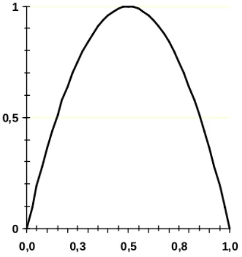
2.1. 1-Dimensional Chaotic Dynamical Systems 2.1.1. Logistic map

The very well known logistic map

g : 0,1

_a

[[[[ ]]]] [[[[ ]]]]

→

0,1

is simply defined as

(((( ))))

((((

))))

a

g

x

=

ax 1

−

x

(1) and generally considered for

a

∈

[[[[ ]]]]

0,4

(see Fig. 1). It is associated to the discrete dynamical system [12]

(((( ))))

n 1 a n

(5)

Singapore (2011) pp. 93-125.

0 0,5 1

0,0 0,3 0,5 0,8 1,0

Figure 1. Graph of the logistic map for

a

====

4

.

This dynamical system which has excellent ergodic properties on the real interval

[[[[ ]]]]

0,1

has been extensively studied especially by R. M. May [13], and J. Feigenbaum [14] who introduced what is now called the Feigenbaum’s constant

δ

====

4.66920160910299067185320382...

explaining by a new theory (period doubling bifurcation) the onset of chaos.

For every value of

a

there exist two fixed points:

x

====

0

which is always unstable and

x

a 1

a

−−−−

====

which is stable for

a

∈

]]]] [[[[

1,3

and unstable for

]]]] [[[[ ]]]] [[[[

a

∈

0,1

∪

1,4

.

When

a

====

4

, the system is chaotic. The set

{{{{

}}}}

5 5 5

5 ,

0.3454915028,0.9045084972

8

8 













₋

₊





====



































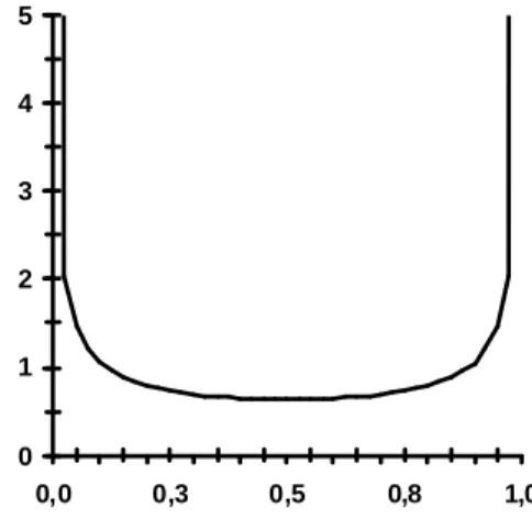
is the period-2

orbit. In fact there exist infinity of periodic orbits and infinity of periods. This dynamical system possesses an invariant measure

P( x )

1 x( 1

x )

π

====

−−−−

(see Fig. 2).

(6)

Singapore (2011) pp. 93-125. 0 1 2 3 4 5 0,0 0,3 0,5 0,8 1,0

Figure 2. Graph of the invariant measure

P( x )

of the logistic map for

a

====

4

. 2.1.2. Numerical approximation of the logistic map

In order to compute longer periodic orbits the use of computer is required, as it is equivalent to find roots of polynomial equation of degree greater than 4 for which Galois theory teaches that no closed formula is available. However, numerical computation uses ordinarily double precision numbers (IEEE-754) so that the working interval contains roughly 1016 representable points. Doing such a computation in Eq. (2) with 1,000 randomly chosen initial guesses, 596, i.e., the majority, converge to the unstable fixed point

x

====

0

, and 404 converge to a cycle of period 15,784,521. (see Table 1) [15].

Table 1. Coexisting periodic orbits found using 1,000 random initial points for double precision numbers

Period Orbit Relative Basin size 1

_x

====

₀

unstable fixed point 596 over 1,000 15,784,521 Scattered over the interval 404 over 1,000

Thus, in this case at least, the very long-term behaviour of numerical orbits is, for a substantial fraction of initial points, in flagrant disagreement with the true behaviour of typical orbits of the original smooth logistic map.

(7)

Singapore (2011) pp. 93-125.

In others numerical experiments we have performed, the computer working with fixed finite precision is able to represent finitely many points in the interval in question. It is probably good, for purposes of orientation, to think of the case where the representable points are uniformly spaced in the interval. The true logistic map is then approximated by a discretized map, sending the finite set of representable points in the interval to itself.

Describing the discretized mapping exactly is usually complicated, but it is roughly the mapping obtained by applying the exact smooth mapping to each of the discrete representable points and "rounding" the result to the nearest representable point. In our experiments [16, 17], uniformly spaced points in the interval with several order of discretization (ranging from 9 to 2,001 points) are involved, the results for 2,000 and 2,001 points are displayed in Table 2. In each experiment the questions addressed are:

• how many periodic cycles are there and what are their periods ?

• how large are their respective basins of attraction, i.e. , for each periodic cycle, how many initial points give orbits with eventually land on the cycle in question ?

Table 2. Coexisting periodic orbits for the discretization with regular meshes of

N

====

2,000 and 2,001

points.

N Period Orbit Relative Basin Size

2,000 1 {0} 2 over 2,000 2,000 2 {1,499} 14 over 2,000 2,000 2 {691;1,808} 138 over 2,000 2,000 3 {276;1,221;1,900} 6 over 2,000 2,000 8 {3;11;43;168;615;1,703.1,008.1,998} 1,840 over 2,000 2,001 1 {0} 5 over 2,001 2,001 1 {1500} 34 over 2,001 2,001 2 {91; 1809} 92 over 2,001 2,001 8 {3;11;43;168;615;1,703;1,011;1,999} 608 over 2,001 2,001 18 {35;137;510;1,519;1,461;1,574;…} 263 over 2,001 2,001 25 {27;106;401;1,282;1,840;588;…} 1,262 over 2,001

The existence of very short periodic orbit (see Table 1), the existence of a non constant invariant measure (see Fig. 2) and the easily recognized shape of the function in the phase space

((((

x , x

_n _{n 1}₊₊₊₊

))))

avoid the use of the logistic map as a PRN generator. However, its very simple implementation in computer program led some authors to use it as a base of cryptosytem [18, 19].

(8)

Singapore (2011) pp. 93-125.

2.1.3. Symmetric tent map

Another often studied dynamical system is defined by the symmetric tent map on the interval

J

= −

[[[[

1,1 ,

]]]]

f : J

_a

→

J

a

f ( x )

= −

1 a x

(3)

(((( ))))

n 1 a n

x

₊₊₊₊

====

f

x

(4)

Despite its simple shape (see Fig. 3), it has several interesting properties. First, when the parameter value

a

====

2

, the system possesses chaotic orbits. Because of its piecewise-linear structure, it is easy to find those orbits explicitly. More, owing to its simple definition, the symmetric tent map’s shape under iteration is very well understood. The invariant measure is the Lebesgue measure. Finally, and perhaps the most important, the tent map is conjugate to the logistic map, which in turn is conjugate to the Hénon map for small values of b [12].

-1 -0,5 0 0,5 1 -1,0 -0,5 0,0 0,5 1,0 Figure 3. Graph of the symmetric tent map on

J

for

a

====

2

.

However the symmetric tent map is dramatically numerically instable: Sharkovskiǐ’s theorem applies for it [20]. When

a

====

2

there exists a period three orbit, which implies that there is infinity of periodic orbits. Nevertheless the orbit of almost every point of the interval

J

of the discretized tent map converges to the (unstable) fixed point

x

= −

1

(this is due to the binary structure of floating points) and there is no numerical attracting periodic orbit [11].

(9)

Singapore (2011) pp. 93-125.

The numerical behaviour of iterates with respect to chaos is worse than the numerical behaviour of iterates of the approximated logistic map. This is why the tent map is never used to generate numerically chaotic numbers. However in Sec. 3 we will show that it is possible to preserve its chaotic properties when several logistic maps are ultra weakly coupled.

2.2. 2-Dimensional System Chaotic Dynamical Systems 2.2.1. Hénon map

In order to study numerically the properties of the Lorenz attractor [11], M. Hénon in 1976 [21] introduced a simplified model of the Poincaré map [12] of this attractor. The Lorenz attractor being in dimension 3, the corresponding Poincaré map is a map from

ℝ

2 to

ℝ

2. The Hénon map is then also defined in dimension 2 as 2

x

y

1 ax

F :

y

bx















_{+ −}



 

→





 

 





(5) It is associated to the dynamical system

2 n 1 n n n 1 n

x

y

1 ax

y

bx

++++ ++++







₌

_{+ −}







====







(6)

For the parameter value

a

====

1.4

,

b

====

0.3

Hénon pointed out numerically that there exists an attractor with fractal structure (see Fig. 4). This was the first example of strange attractor (previously introduced by D. Ruelle and F. Takens [22]) for a mapping defined by an analytic formula.

Nowadays hundreds of research papers have been published on this prototypical map in order to fully understand its innermost structure. However as in dimension 1, there is a discrepancy between the mathematical properties of this map in the plane

ℝ

2 and the numerical computations done using (IEEE-754) double precision numbers.

If we call Megaperiodic orbits [23], those whose length of the period belongs to the interval of natural numbers



_



10 ,10

6 9



_



_

and Gigaperiodic orbits, those whose length of the period belongs to the interval



_



10 ,10

9 12



_



_

, Hénon map possesses Gigaperiodic orbits. On a Dell computer with a Pentium IV microprocessor running at the frequency of 1.5 Gigahertz, using a Borland C compiler and computing with ordinary (IEEE-754) double precision numbers, one can find for

a

====

1.4

and

b

====

0.3

one attracting period of length 3,800,716,788

(10)

Singapore (2011) pp. 93-125.

i.e. two hundred forty times longer than the longest period of the one-dimensional

logistic map (see Table 1).

Figure 4. The strange attractor of the Hénon map for

a

====

1.4

and

b

====

0.3

. This periodic orbit (we call it here Orbit 1) is numerically slowly attracting. Starting with the initial value

(x0 , y0)1 = (-0.35766, 0.14722356) one obtains:

(x11,574,730,767 , y11,574,730,767)1 = (x15,375,447,555 , y15,375,447,555)1

= (1.27297361350955662, – 0.0115735710153616837) The length of the period is obtained subtracting

15,375,447,555 – 11,574,730,767 = 3,800,716,788. However this periodic orbit is not unique: starting with the initial value

(x0 , y0)2 = (0.4725166, 0.25112222222356) the following periodic orbit (which is

a Megaperiodic orbit of period 310,946,608 (Orbit 2)) is computed. (x12,935,492,515, y12,935,492,515)2 = (x13,246,439,123, y13,246,439,123)2

= (1.27297361350865113, – 0.0115734779561870744) This orbit can be reached more rapidly starting form the other initial value

(x0, y0) = (0.881877775591, 0.0000322222356), then

(x4,459,790,707, y4,459,790,707) = (1.27297361350865113, – 0.0115734779561870744). It is possible that some others periodic orbits coexist with both Orbit 1 and Orbit 2.

The comparison between Orbit 1 and Orbit 2 gives a perfect idea of the sensitive dependence on initial conditions of chaotic attractors: Orbit 1 passes

(11)

Singapore (2011) pp. 93-125.

through the point (1.27297361350955662, – 0.0115735710153616837) and Orbit 2 passes through the point (1.27297361350865113, – 0.0115734779561870744). The same digits of these points are bold printed, they are very close.

Nevertheless, as displayed in Fig. 4 the orbit are not uniformly distributed on the phase space, then it is not possible to use this map as a PRN generator.

Beside the problem of PRN generator, logistic and Hénon maps are recently used together with a secret key, by N. Pareek et al. [24], in order to build a chaotic block cipher which is extremely robust, due to the excellent confusion and diffusion properties of these maps. The results of the statistical analysis show that the chaotic cipher possesses all features needed for a secure system and useable for the security of communication system.

L. dos Santos Coelho et al. [25], introduced a chaotic particle swarm optimisation (PSO) which is a population-based swarm intelligence algorithm driven by the stimulation of a social psychological metaphor instead of the survival of the fittest individual. Based on the chaotic systems theory (using Hénon map sequences which increase its convergence rate and resulting precision) the novel PSO combined with an implicit filtering allows solving economic dispatch problems.

2.2.2. Lozi map

The Lozi map [26] is a linearized version of the Hénon map, built in order to simplify the computations, mainly because it is possible to compute explicitly any periodic orbits solving a linear system. It is defined as

n 1 n n n 1 n

x

y

1 a x

y

bx

++++ ++++







₌

_{+ −}







====







(7) or equivalently n 1 n n 1

x

₊₊₊₊

= −

1 a x

+

bx

₋₋₋₋ (8)

For

a

====

1.7

and

b

====

0.5

there exists a strange attractor. The particularity of this strange attractor is that it has been rigorously proved by Misiurewicz in 1980 [27].

In the same conditions of computation as for Hénon map, running the computation during nineteen hours, one can find a Gigaperiodic attracting orbit of period 436,170,188,959 more than one hundred times longer than the period of Orbit 1 found for the Hénon map.

(12)

Singapore (2011) pp. 93-125.

Starting with (x0, y0) = (0.88187777591, 0.0000322222356) one obtains

(x686,295,403,186 , y686,295,403,186) = (x250,125,214,227 , y250,125,214,227)

= (1.34348444450739479, -2.07670041497986548. 10-7).

There is a transient regime before the orbit is reached. It seems that there is no periodic orbit with a smaller length. This could be due to the quasihyperbolic nature of the attractor. However, the orbit-shifted shadowing property of Lozi map (and generalized Lozi map), which is the property which ensures that pseudo-orbits of a homeomorphism

f

can be traceable by actual orbits even if rounding errors in computing are not inevitable has been recently proved [28].

Hence this attractor is very efficient, in order to generate chaotic numbers without repetition for standard simulation using either the first or the second component. However they are not equally distributed on the plane (see Fig. 5). The non constant density forbids its direct use as a PRN generator. Nevertheless there are some U.S. patents for “method of generating pseudo-random numbers in an electronic device, and a method of encrypting and decrypting electronic data” in which the Lozi map is involved [29, 30].

Figure 5. Invariant density of the second component

y

of Eq. (7) computed using 1010 iterations.

Nevertheless Lozi map is now widely used in chaotic optimisation which belongs to a new class of algorithms: the evolutionary algorithms (EA). In a

0 0,2 0,4 0,6 0,8 1 1,2 1,4 1,6 1,8 2 -0,68 -0,49 -0,29 -0,09 0,1 0,3 0,5 0,68

(13)

Singapore (2011) pp. 93-125.

founding paper, R. Caponetto et al. [31] propose an experimental analysis on the convergence of EA. The effect of introducing chaotic sequences instead of random ones during all the phases of the evolution process is investigated. The approach is based on the substitution of the PRNG with chaotic sequences. Several numerical examples are reported in order to compare the performance of the EA using random and chaoticgenerators as regards to both the results and the convergence speed. The results obtained show that chaotic sequences obtained from Lozi map are always able to increase the value of some measured algorithm-performance indexes with respect to random sequences.

Several authors following this idea use Lozi map in chaotic optimization in order to avoid local optima stagnation and embed a superior search strategy [32 – 40].

2.3. 3-Dimensional System Chaotic Dynamical Systems

In order to generalize in higher dimension the tent map, G. Manjunath et al. [41] introduce a three-dimensional map

F : I

3

→

I

3where

I

====

[[[[ ]]]]

0,1

(see Fig. 6) which is continuous in the Euclidian topology and prove its chaotic properties:

y

z

1 2x

1

2 x

z

F( x, y, z )

1 2 y

1

2 x

y

1 2z

1

2 













₊₊₊₊



−

+

−

+

−

+

−

+

−















































₊₊₊₊



















=

−

+

−

=

−

+

−

=

−

+

−

=

−

+

−

































++++















₋

₊

₋



































(9)

The related dynamical system is

((((

x

n 1++++

, y

n 1++++

,z

n 1++++

,

))))

====

F x , y , z ,

((((

n n n

))))

(10)

They emphasize that most of the well known examples of higher dimensional chaotic dynamical systems belong to the class of hyperbolic diffeomorphisms on a

n-torus. These higher dimensional maps on the torus are not continuous on the

standard topology of the Euclidean space since they exhibit jump discontinuities. The realization of such jump discontinuities in an electronic circuit implementation is not reliable. They prove the following theorem:

(14)

Singapore (2011) pp. 93-125.

Theorem (G. Manjunath et al.) The map defined in (9) is topologically transitive and exhibits sensitive dependence on initial conditions with any real number

0,

3

2 δ

∈



_



_



_







_



_



_







_



_





















as sensitivity constant.

Once again the sequence of iterated points

((((

x , y ,z

_n _n _n

))))

obtained from the dynamical system (10) is not equally distributed on the volume

I

3. The invariant density of the first component

x

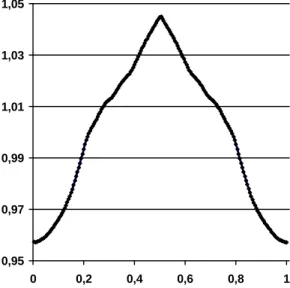
_n is displayed in Fig. 7. The relative discrepancy of this invariant density versus the uniform one lies between 4% and 5%.

Figure 6. Tessellation of

I

3 into 33 regions by parallel set of critical planes

y ,z

T

( z )

====

0 and 1

,

T

x ,z

( y )

====

0 and 1

,

T

x ,z

( z )

====

0 and 1

, pertaining

to the map (9).

To allow the generation of PRN using complexity and emergence theory we consider in the next section how to generate these numbers with uniform repartition on a given interval, or on a given square of the plane or more generally in a given hypercube of

ℝ

n involving the ultra weak multidimensional coupling of p 1-dimensional chaotic dynamical systems.

(15)

Singapore (2011) pp. 93-125. 0,95 0,97 0,99 1,01 1,03 1,05 0 0,2 0,4 0,6 0,8 1

Figure 7. Invariant density of the first component

x

of Eq. (10) computed using 1011 iterations.

3. Multi-parameter Chaotic Pseudo-Random Number Generator (M-p CPRNG)

As previously seen, when a dynamical system is realized on a computer using floating point or double precision numbers, the computation is of a discretization, where finite machine arithmetic replaces continuum state space. For chaotic dynamical systems, the discretization often has collapsing effects to a fixed point or to short cycles [15, 42]. In order to preserve the chaotic properties of the continuous models in numerical experiments we consider an ultra weak multidimensional coupling of p one-dimensional dynamical systems.

3.1. System of p-Coupled Symmetric Tent Map

In order to simplify the presentation of the M-p CPRNG we introduce, we use as an example the symmetric tent map previously defined (3), even though others chaotic map of the interval (as the logistic map, the baker transform, …) can be used for the same purpose (as a matter of course, the invariant measure of the chaotic map chosen is preserved).

(16)

Singapore (2011) pp. 93-125.

(((( ))))

((((

))))

n 1 n n

X

₊₊₊₊

=

F X

= ⋅

A

f ( X )

(11) with 1 1

(

)

,

(

)

(

)

n n n n p p n n

x

f x

X

f X

x

f x

⋮

















=





=





















(12) and 1,1 1, 2 2,2 2, 1, 2 1 , , 1 j p j 1,2 1,p-1 1,p j j p 2,1 j 2,p-1 2,p j j j p p,1 p,p-1 p p p j j

=1-

ε

_=1-

ε

A

ε

_=1-

ε

⋯

⋮

⋱

⋮

⋱

⋮

⋯

= = = = ≠ = − =

























=

_

_

























∑

(13)

F

is a map of

J

p

= −

[ ]

1,1

p

⊂

ℝ

p into itself.

Considering j p i , i i , j j 1, j i

=

1-ε

=

ε

=

∑

≠

, the matrix A is always a stochastic matrix iff the coupling constants verify

ε

_{i , j}

>

0

for every i and j.

If _{i, j}

i j

i,j

ε

₀

≠

∀

=

the maps are totally decoupled, instead they are fully crisscross coupled when for example _{i, j}

i j

1 ε

p

1

≠

=

−

. Generally, researchers do not consider very small values of

ε

_{i j}_, because it seems that the maps are quasi-decoupled with those values and no special effect of the coupling is expected. In fact it is not the case and ultra small coupling constants (as small as 10-7 for floating point numbers or 10-16 for double precision numbers), allows the construction of very long periodic orbits, leading to sterling chaotic generators. This is the way in complexity leads to randomness from chaos.

(17)

Singapore (2011) pp. 93-125.

Moreover each component of these numbers belonging to

ℝ

p is equally distributed over the finite interval

J

⊂

ℝ

, when one chooses a function f with uniform invariant measure. Numerical computations (up to 1013 numbers) show that this distribution is obtained with a very good approximation. They have also the property that the length of the periods of the numerically observed orbits is very large [23].

3.2. Chaotic Sampling and Mixing

However chaotic numbers are not pseudo-random numbers because the plot of the couples of any component

((((

x , x

l_n l_{n 1}₊₊₊₊

))))

of iterated points

(

X

_n

,

X

_n₊₁

)

in the corresponding phase plane reveals the map f used as one-dimensional dynamical systems to generate them via Eq. (11).

Nevertheless we have recently introduced a family of enhanced Chaotic Pseudo Random Number Generators (CPRNG) in order to compute very fast long series of pseudorandom numbers with desktop computer [3, 4, 5]. This family is based on the previous ultra weak coupling which is improved in order to conceal the chaotic genuine function.

In order to hide f in the phase space

(

x , x

_nl _{n 1}l₊

)

two mechanisms are used. The pivotal idea of the first one mechanism is to sample chaotically the sequence

((((

l l l l l

))))

0 1 2 n n 1

x , x , x ,

…

, x , x

₊₊₊₊

,

…

generated by the l-th component

x

l, selecting

l n

x

every time the value

x

_nm of the m-th component

x

m, is strictly greater (or smaller) than a threshold

T

∈

J

, with l ≠ m, for 1 ≤ l, m ≤ p.

That is to say to extract the subsequence

(

( 0 )

,

(1)

,

( 2 )

,

( )q

,

(q1)

,

)

l l l l l

n n n n n

x

…

x

…

+ denoted here

((((

x , x , x ,

0 1 2

⋯

, x , x

q q 1++++

,

⋯

))))

of the original one, in the following way

Given

1 ≤

l m

,

≤

p l

,

≠

m

{

}

( ) ( 1) ( ) ( 1)

1 ,

q l m q n q q r r

n

x

with n

Min r

n

x

T

ℕ − − ∈

= −





=

>



(14)

(18)

Singapore (2011) pp. 93-125.

The sequence

((((

x , x , x ,

₀ ₁ ₂

⋯

, x , x

_q _{q 1}₊₊₊₊

,

⋯

))))

is then the sequence of chaotic pseudo-random numbers.

The mathematical formula (14) can be best understood in algorithmic way. The pseudo-code, for computing iterates of (14) corresponding to N iterates of (11) is:

(

1 2 p 1 p

)

0 0 0 0 0

X

=

x , x ,

…

, x

−

, x

=

seed

n

=

0; q

=

0

do

{

while n < N do

{

while

(

x

_nm

≤

T

)

compute

(

x , x ,

_n1 _n2

…

, x

_np 1−

, x

_np

)

; n + +

}

compute

(

x , x ,

_n1 _n2

…

, x

_np 1−

, x

_np

)

; then ( )q l q n

n( q )

=

n ;

x

=

x

;

n + +; q + +

}

This chaotic sampling is possible due to the independence of each component of the iterated points

X

_n vs. the others [3].

Remark 1: Albeit the number

NSampl

_iter of pseudo-random numbers

q

x

corresponding to the computation of N iterates is not known a priori, considering that the selecting process is again linked to the uniform distribution of the iterates of the tent map on

J

, this number is equivalent to

2

1 N

T

−

.

A second mechanism can improve the unpredictability of the pseudo-random sequence generated as above, using synergistically all the components of the vector

X

_n, instead of two. Given p - 1 thresholds

1 2 p 1

T

<

T

<

⋯

<

T

₋

∈

J

(15) and the corresponding partition of

J

1 0 p k k

J

∪

J

− =

=

(16)

with

J

₀

= −

[

1,T

₁

]

,

J

₁

=

]

T ,T

₁ ₂

[

,

J

_k

=

[

T ,T

_k _k₊₁

[

for

1 < < −

k

p

1

and

1 1

1

p p

J

₋₋₋₋

====



_



_



_

T

₋₋₋₋

,

_



_



, this simple mechanism is based on the chaotic mixing of the

(19)

Singapore (2011) pp. 93-125.

((((

1 1 1 1 1

))))

0 1 2 n n 1

x , x , x ,

…

, x , x

₊₊₊₊

,

…

,

((((

x , x , x ,

₀2 ₁2 2₂

…

, x , x

_n2 _{n 1}2₊₊₊₊

,

…

))))

,…,

((((

x

₀p 1−−−−

, x

₁p 1−−−−

, x

₂p 1−−−−

,

…

, x

_np 1−−−−

, x

_{n 1}p 1₊₊₊₊−−−−

,

…

))))

,…

using the last one

((((

x , x , x ,

₀p ₁p ₂p

…

, x , x

_np _{n 1}p₊₊₊₊

,

…

))))

in order to distribute the iterated points with respect to this given partition defining the subsequence

(

( 0 )

,

(1)

,

( 2 )

,

( )q

,

(q1)

,

)

l l l l l n n n n n

x

…

x

…

+ here denoted

((((

x , x , x ,

0 1 2

⋯

, x , x

q q 1++++

,

⋯

))))

by

{

}

{

}

( q ) k k ( 1 ) k p q n ( q ) k k ( q 1 ) r k 1 k p 1 r

n

1 x

x

, with n

Min s ( q )

Min r

n

x

J

ℕ − − ≤ ≤ − ∈

= −







=

>

∈



(17)

The pseudo-code, for computing the iterates of (17) corresponding to N iterates of (11) is:

(

1 2 p 1 p

)

0 0 0 0 0

X

=

x , x ,

…

, x

−

, x

=

seed

n

=

0; q

=

0

do

{

while n < N do

{

while

(

x

_np

∈

J

₀

)

compute

(

x , x ,

1_n _n2

…

, x

_np 1−

, x

_np

)

; n + +

}

compute

(

x , x ,

1_n _n2

…

, x

_np 1−

, x

_np

)

let k be such that

x

_np

∈

J

_k

then

( )q

k

q n

n( q )

=

n ;

x

=

x

; n + +; q + +

}

Remark 2: In this case also,

NSampl

_iter is not known a priori, however, considering that the selecting process is linked to the uniform distribution of the iterates of the tent map on

J

, one has

1

2

1

iter

N

NSampl

T

≈

−

.

(20)

Singapore (2011) pp. 93-125.

Remark 3: This second mechanism is more or less linked to the whitening process [43, 44].

Remark 4: Actually, one can choose any of the components in order to sample and mix the sequence, not only the last one.

3.3. Double Threshold Chaotic Sampling

On can eventually improve the CPRNG previously introduced with respect to the infinity norm instead of the

L

₁ or

L

₂ norms because the

L

_∞ norm is more sensitive than the others ones to reveal the concealed function f [5]. For this purpose we introduce a second kind of threshold

T

'

∈

ℕ

, together with

1

,

p 1

T

⋯

T

₋

∈

J

such that the subsequence

((((

x , x , x ,

₀ ₁ ₂

⋯

, x , x

_q _{q 1}₊₊₊₊

,

⋯

))))

is defined by

{

}

{

}

( q ) k k ( 1 ) k p q n ( q ) k k ( q 1 ) r k 1 k p 1 r

n

1 x

x

, with n

Min s ( q )

Min r

n

T '

x

J

ℕ − − ≤ ≤ − ∈

= −







=

>

+

∈



(18) In pseudo-code Eq. (18) is then:

(

1 2 p 1 p

)

0 0 0 0 0

X

=

x , x ,

…

, x

−

, x

=

seed

n

=

0, q

=

0

do

{

while n < N do

{

while

(

n

≤

n

_{( q 1 )}₋

+

T '

and

x

_np

∈

J

₀

)

compute

(

x , x ,

1_n _n2

…

, x

_np 1−

, x

_np

)

; n + +

}

compute

(

x , x ,

_n1 _n2

…

, x

_np 1−

, x

_np

)

let k be such that

x

_np

∈

J

_k

then

( )q

k

q n

n( q )

=

n ;

x

=

x

; n + +; q + +

}

Remark 5: In this case also,

NSampl

_iter is not known a priori, it is more complicated to give an equivalent to it. However, considering that the selecting

(21)

Singapore (2011) pp. 93-125.

process is linked to the uniform distribution of the iterates of the tent map on

J

, and to the second threshold T’, it comes that

1

2 ,

1

iter

N

NSampl

Min

T T





≤





′

−





.

Remark 6: the second kind of threshold

T

'

can also be used with only the chaotic sampling, without the chaotic mixing.

4. Emergence of Randomness

Numerical results about chaotic numbers produced by (11) — (17) show that they are equally distributed over the interval

J

with a very good precision [3, 4]. In this section we emphasize that when the parameters

ε

_{i j}_, belong to a special window (called the window of emergence) the M-p CPRNG defined above behaves well.

4.1. Approximated Invariant Measures

In order to perform numerical computation, we have to define some numerical tools: the approximated invariant measures.

First we define an approximation

P

_{M N}_,

( )

x

of the invariant measure also called the probability distribution function linked to the 1-dimensional map f when computed with floating numbers (or numbers in double precision). In this scope we consider a regular partition of M small intervals (boxes) ri of

J

defined by:

i 2i s 1 , i 0, M M = − + = i i i 1 r = s , s ₊  , i = 0, M - 2

[

]

M 1 M 1

r

₋

=

s

₋

, 1

1 0 M i

J

∪

r

−

=

the length of each box is

i 1 i

2 s

s

M

++++

− =

(note that this regular partition of

J

is different from the previous one linked to the threshold values

T

_i (16)).

All iterates f (n)(x) belonging to these boxes are collected (after a transient regime of Q iterations decided a priori, i.e. the first Q iterates are neglected). Once

(22)

Singapore (2011) pp. 93-125.

the computation of N + Q iterates is completed, the relative number of iterates with respect to N/M in each box ri represents the value

P s

N

( )

i . The approximated

( )

N

P x

defined in this article is then a step function, with M steps. As M may vary, we define

( )

,

( )

#

M N i i

1 M

P

s

r

2 N

=

where #ri is the number of iterates belonging to the interval ri and the constant 1/2

allows the normalisation of

P

_{M ,N}

( x )

on the interval

J

.

M ,N M ,N i i

P

( x )

=

P

( s )

∀ ∈

x

r

In the case of p-coupled maps, we are more interested by the distribution of each component

(

x

1

,

x

2

,

x

₂1

,

…

,

x

p

)

of X rather than the distribution of the variable X itself in

J

p . We then consider the approximated probability distribution function

P

_{M N}_,

(

x

j

)

associated to one among several components of

F(X) defined by (11) which are one-dimensional maps. In this paper we use

equally

N

_disc for M and

N

_iter for N when they are more explicit.

The discrepancies

E

₁ (in norm

L

₁),

E

₂ (in norm

L

₂) and

E

_∞ (in norm

L

_∞) between

disc iter

N , N

P

( x )

and the Lebesgue measure which is the invariant measure associated to the symmetric tent map, are defined by

1

1,N_disc,N_iter

( )

N_disc,N_iter

( )

0.5

_L

E

x

=

P

x

−

2

2,Ndisc,Niter

( )

Ndisc,Niter

( )

0.5

_L

E

x

=

P

x

−

,N_disc,N_iter

( )

N_disc,N_iter

( )

0.5

_L

E

x

P

x

∞

=

−

In the same way an approximation of the correlation distribution function

,

( , )

M N

C

x y

is obtained numerically building a regular partition of

M

2 small squares (boxes) of

J

2 imbedded in the phase subspace (xl, xm)

,

i j

2i

2 j

s

1 t

1 i j

0 M

M

= − +

=

i , j i i 1 j j 1

0, M-2

r

=

s , s



_

₊₊₊₊

_{ }



_



_



_



×

t , t

_



_



_



₊₊₊₊

_



_



_

, i, j

=

[

[ [

]

i ,M 1 i i 1 M 1

r

₋

=

s , s

₊

×

t

₋

, 1 , j

=

0, M-2

(23)

Singapore (2011) pp. 93-125.

[

] [

]

M 1,M 1 M 1 M 1

r

₋ ₋

=

s

₋

, 1

×

t

₋

, 1

the measure of the area of each box is

((((

i 1 i

)))) ((((

i 1 i

))))

2

2 s

s

t

M

+ + + + + + + +













−

×

−

=

−

×

−

=

−

×

−

=

















Once N + Q iterated points

((((

x , x

_nl _nm

))))

belonging to these boxes are collected the relative number of iterates with respect to N/M2 in each box ri,j represents the

value CN (si,tj). The approximated probability distribution function CN (x,y)

defined here is then a 2-dimensional step function, with M 2 steps. As M can take several values in the next sections, we define

(((( ))))

2 M ,N i j i , j

1 M

C

( s , t )

# r

4 N

====

(19)

where #ri,j is the number of iterates belonging to the square ri,j and the constant 1/4

allows the normalisation of

C

_{M ,N}

( x, y )

on the square

J

2

M ,N M ,N i j i , j

C

( x, y )

=

C

( s ,t )

∀

( x, y )

∈

r

(20) The discrepancies 1 C

E

(in norm

L

₁), 2 C

E

(in norm

L

₂) and

E

_C

∞ (in norm

L

_∞) between

disc iter

N , N

C

( x, y )

and the uniform distribution on the square, are defined by

1

, _disc, _iter

( , )

_disc, _iter

( , )

0.25

C N N N N _L

E

x y

=

C

x y

−

2

, disc, iter

( , )

disc, iter

( , )

0.25

C N N N N _L

E

x y

=

C

x y

−

, _disc, _iter

( , )

_disc, _iter

( , )

0.25

C N N N N _L

E

_∞

x y

C

x y

∞

=

−

Finally let disc iter N , N

AC

( x, y )

be the autocorrelation distribution function which is the correlation function

disc iter

N , N

C

( x, y )

of (20) defined in the phase space

((((

x , x

_nl _{n 1}l₊₊₊₊

))))

instead of the phase space

(

xl,xm

)

. In order to control that the enhanced chaotic numbers

((((

x , x , x ,

₀ ₁ ₂

⋯

, x , x

_q _{q 1}₊₊₊₊

,

⋯

))))

are uncorrelated, we plot them in the phase subspace

((((

x , x

_q _{q 1}₊₊₊₊

))))

and we check if they are uniformly distributed in the square

J

2 and if f is concealed (i.e.

(24)

Singapore (2011) pp. 93-125.

1, disc, iter

(

,

1

),

2, disc, iter

(

,

1

),

AC N N q q AC N N q q

E

x x

₊

E

x x

₊ _, _,

(

,

₁

)

disc iter AC N N q q

E

_∞

x x

₊ vanish).

4.2. A window of Emergence of Randomness

In order to point out the usefulness of the double threshold chaotic sampling with simply consider the case of only 4 coupled equations, and such that

ε

_{i , j}

=

ε

_i

∀ ≠

i

j

and

ε

_{i , i}

= 1-3

ε

_i. Eq. (11) becomes

1 1 2 3 4 n 1 1 n 1 n 1 n 1 n 2 1 2 3 4 n 1 2 n 2 n 2 n 2 n 3 1 2 3 4 n 1 3 n 3 n 3 n 3 n 4 1 2 3 4 n 1 4 n 4 n 4 n 4 n

x

( 1

3 ε ) f ( x )

ε

_{f ( x )}

ε

_{f ( x )}

ε

_{f ( x )}

x

ε

_{f ( x ) ( 1}

_{3 ε ) f ( x )}

ε

_{f ( x )}

ε

_{f ( x )}

x

ε

_{f ( x )}

ε

_{f ( x ) ( 1}

_{3 ε ) f ( x )}

ε

_{f ( x )}

x

ε

_{f ( x )}

ε

_{f ( x )}

ε

_{f ( x ) ( 1}

_{3 ε ) f ( x )}

++++ ++++ ++++ ++++







₌

₋

₊







=

+ −

+

=

+ −

+

=

+ −

+













=

+

+ −

+

=

+

+ −

+

=

+

+ −

+

=

+

+ −

+











₌

₊

_{+ −}







(21)

Moreover we assume that

ε

_i

====

_{i ε}

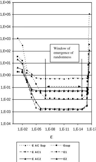
₁

For the shake of simplicity we consider only the chaotic sampling method (i.e. we use only one threshold