HAL Id: halshs-01535161
https://halshs.archives-ouvertes.fr/halshs-01535161
Submitted on 8 Jun 2017
HAL is a multi-disciplinary open access archive for the deposit and dissemination of sci-entific research documents, whether they are pub-lished or not. The documents may come from teaching and research institutions in France or abroad, or from public or private research centers.
L’archive ouverte pluridisciplinaire HAL, est destinée au dépôt et à la diffusion de documents scientifiques de niveau recherche, publiés ou non, émanant des établissements d’enseignement et de recherche français ou étrangers, des laboratoires publics ou privés.
Price elasticities for disaggregated expenditures
François Gardes
To cite this version:
Documents de Travail du
Centre d’Economie de la Sorbonne
Price elasticities for disaggregated expenditures
François GARDES
Price elasticities for disaggregated expenditures
François Gardes, Paris School of Economics, Université Paris I Panthéon-Sorbonne, CES1
Abstract
The relation between price elasticities computed at different levels of aggregation is a prominent question in the evaluation of price effects in the empirical literature on households’ consumption, production or international trade. We propose to model it under a strong separability assumption in order to estimate price elasticities at a disaggregated level when only price aggregates are available in the dataset. The estimation of price elasticities for aggregate consumptions uses an original domestic production model combining monetary expenditures and time uses for aggregate activities in order to calculate full prices of these aggregates. The method is applied for food expenditures on surveys of two different countries, France and Burkina Faso.
JEL classification: C33, D1, D13, J22
Keywords: domestic production, full price, price elasticity, Pigou law.
1. Introduction
Micro-simulation exercises often oblige to calibrate income and price effects at a precise level of the expenditures than what is available in the dataset, for instance for alcoholic beverages when a specific tax is applied to them. Suppose this specific item i is included in the broad consumption activity (named semi-aggregate commodity) I (food). The total expenditure for the semi-aggregate commodity I writes: 𝑃𝐼𝑋𝐼 = ∑𝑖∈𝐼𝑝𝑖𝑥𝑖 with 𝑃𝐼 and 𝑋𝐼 the price and quantity aggregates for I. Income elasticities could be estimated by means of the estimation of demand equations for disaggregate items of a semi-aggregate expenditure (using for all demand functions the price index of the broad category to which this item pertains). For such a demand function, biases may occur in the estimation of the income coefficient only in the unlikely case where the price of the broad category is correlated to income, while the specific price for the disaggregate item is not.
As far as price effects are concerned, own price elasticities for individual items within the semi-aggregate consumption I may be estimated using the price index of the broad activity 𝑃𝐼. But this would suppose that all the variations in the individual price pi of the specific
expenditure i are reflected in the variations of 𝑃𝐼 (which, for instance, is not the case for
1 François Gardes, Maison des Sciences Economiques, 106-112 Boulevard de l’Hôpital, 75647, Paris cedex 13.
Courriél: [email protected]; tél. 01 44 07 82 87.
Acknowledgment to the General Directorate for the Promotion of the Rural Economy (DGPER) and the University of Ouaga II and to INSEE for the disposition of its Family Expenditures and Time-Use surveys, and to Christophe Starzec and Noël Thiombiano for their collaboration in the preparation of these datasets.
changes in special taxations on goods or services such as tobacco or restaurants). Moreover, the substitutability or complementarity between disaggregate consumptions inside the semi-aggregate I can only be estimated by means of individual prices for these dissemi-aggregate items. We propose in this article to examine the relation between the own-price elasticity of the aggregate (which depends on all own and cross-price of the items composing the aggregate) and those of the items within this aggregate. Even when data are available on individual prices, differences between the price elasticity of the aggregate and the average of the price elasticities of these items may arise through the substitution and complementarities between these items, which are difficult to estimate. That problem has been well documented as concerns for instance elasticities of imports and exports. Our method is based on the assumption that the structure of price-elasticities for sub-categories calculated under strong separability indicates the true structure of these elasticities, which is supported by the estimation on French data. The estimation of the own price-elasticities for the aggregate serves as an average values over which these disaggregated elasticities are calibrated.
The own-price elasticities of semi-aggregate consumptions such as Food, Transportation or Leisure activities are estimated over full prices which are calculated with an opportunity cost of time estimated using households’ monetary expenditures and Time Uses. In one country, the Burkina Faso, both informations are known in the survey over rural households. In France, a Family Expenditure survey, containing monetary expenditures, is matched with a Time Use survey in order to recover time use for each household of the Family Expenditure survey. Both dataset furnish significant and negative own-price elasticities of 3 to 8 semi-aggregate consumptions.
Section 1 defines the price index for the semi-aggregate expenditure I. Section 2 analyses the relation between price elasticities for the semi-aggregate and the individual items of expenditures. Section 3 presents a method to estimate price elasticities for broad consumption activities using a domestic production framework and section 4 applies the method to a French dataset and a Burkina Faso survey.
Section 1. Relation between aggregate and disaggregate price elasticities
First, in order to calculate price elasticities for disaggregate items, we define the price index 𝑃𝐼 for the broad consumption activity I as a true cost-of-living index proportional to the cost function C(p,u)2 for consumption I: 𝑃
𝐼 = 𝑘𝐶(𝑝, 𝑢). This cost corresponds to the
expenditure for prices p at the constant utility level u: 𝐶(𝑝, 𝑢) = ∑𝑖∈𝐼𝑝𝑖𝑞𝑖 for the Hicksian
demand functions 𝑥𝑖 = ℎ𝑖(𝑝, 𝑢). Using the Shephard lemma to calculate the hicksian demand we obtain the elasticity of the aggregate price 𝑃𝐼 over the individual price 𝑝𝑖 as:
𝐸𝑃𝐼/𝑝𝑖 = 𝜕𝑙𝑛𝑃𝐼 𝜕𝑙𝑛𝑝𝑖 = 𝑘𝜕𝐶 𝜕𝑝𝑖 𝑝𝑖 𝑘𝐶= 𝑝𝑖𝑥𝑖 𝑃𝐼𝑋𝑖= 𝑤𝑖/𝐼 (1)
2 We make here the assumption of a strong separability between expenditures in different semi-aggregate
commodities, so that the utility level in this cost function depends only on consumptions in the group I. Another way would be to consider that this utility is conditional to all other expenditures in other broad groups.
where 𝑤𝑖/𝐼 is the budget share of item i in its semi-aggregate group I, so that the logarithmic price index can be written as an Aftalion-Stone index: 𝑙𝑛𝑃𝐼= 𝑎𝐼+ ∑𝑖∈𝐼𝑤𝑖/𝐼𝑙𝑛𝑝𝑖.
Second, in order to establish a relationship between the own-price elasticity of the semi-aggregate expenditure and elasticities of individual expenditures, we calculate the derivative of the average aggregate expenditure over its average aggregate price3. As the price index P
I
is a geometric mean of individual prices in group I, the average quantity XI must also be a
geometric mean of individual consumptions xi so that the value of the semi-aggregate
expenditure writes also as a geometric mean of individual expenditures. The average semi-aggregated quantity thus writes 𝑋̅ = ∏𝐼 𝑥𝑖𝑤𝑖/𝐼
𝑖∈𝐼 and the value of the semi-aggregated
expenditure I is: 𝑃𝐼𝑋𝐼 = (𝑃𝐼𝑋̅ )𝐼 𝑁𝐼 = ∏ (𝑝
𝑖𝑥𝑖)𝑁𝐼𝑤𝑖/𝐼
𝑖∈𝐼 with 𝑁𝐼 the number of consumption
items in the semi-aggregate group I and 𝑁𝐼𝑤𝑖/𝐼 the total weight of item i in the semi-aggregate I such as 𝑁𝐼 = ∑ 𝑁𝐼𝑤𝑖
𝐼 ⁄
𝑖∈𝐼 . The price elasticity of this average expenditure is:
𝜕𝑙𝑛𝑃𝐼𝑋̅̅̅𝐼 𝜕𝑙𝑛𝑃𝐼 = 1 𝑁𝐼∑𝑖∈𝐼𝑤𝑖/𝐼 𝜕𝑙𝑛𝑝𝑖𝑥𝑖 𝜕𝑙𝑛𝑃𝐼 = 1 𝑁𝐼∑𝑖,𝑗∈𝐼𝑤𝑖/𝐼 𝜕𝑙𝑛𝑝𝑖𝑥𝑖 𝜕𝑙𝑛𝑝𝑗 𝜕𝑙𝑛𝑝𝑗 𝜕𝑙𝑛𝑃𝐼= 1 𝑁𝐼∑ 𝑤𝑖∈𝐼 𝑤𝑗∈𝐼𝐸𝑖𝑗 𝑖,𝑗∈𝐼 (2)
where 𝐸𝑖𝑗 is the cross-price elasticity of the individual consumption for item i on price 𝑝𝑗 and 𝑤𝑖 and 𝑤𝑗 the budget shares of consumptions i and j over total expenditure.
Third, we assume that individual expenditures are strongly separable within the semi-aggregates and that these semi-semi-aggregates are also separable between them (which amounts to suppose that all individual expenditures are separable). This hypothesis allows computing direct and cross-price elasticities by means of the Frisch formula:
𝐸𝑖𝑗 = Ф𝐸𝑖𝛿𝑖𝑗− 𝐸𝑖𝑤𝑗(1 + Ф𝐸𝑗) (3)
Here Ф is the Frisch income flexibility and 𝐸𝑖 the income-elasticity for good i. Finally, we normalize these disaggregated price elasticities by multiplying them by the ratio of the aggregate elasticity on the left term of equation (2) over the sum of individual elasticities on the right, in order to define price elasticities verifying this additivity constraint.
Re-writing equation (2) for these disaggregated elasticities gives:
E𝑃𝐼𝑋𝐼/𝑃𝐼 = 1 𝑁𝐼∑ 𝑤𝑖,𝐼 𝑤𝑗,𝐼𝐸𝑖𝑗 i,j = Ф 𝑁𝐼∑ 𝐸𝑖 𝑖 − 1 𝑁𝐼∑ ∑ 𝑤𝑖/𝐼 𝑗∈𝐼 𝐸𝑖 𝑗 − Ф 𝑁𝐼∑[∑ 𝑤𝑗/𝐼 𝑗∈𝐼 𝐸𝑗]𝐸𝑖 𝑖 = Ф 𝑁𝐼{1 − 𝑤𝐼𝐸𝐼/𝑌} ∑ 𝐸𝑖 𝑖∈𝐼 − 1 𝑁𝐼𝑤𝐼𝐸𝐼/𝑌 = 𝐴 (4)
3 We restrict the analysis to the case where no substitution or complementarity exist between item pertaining to
with 𝐸𝑖𝑗 = Epixi/pj, 𝑤𝑖/𝐼= 𝑝𝑖𝑥𝑖
∑𝑖∈𝐼𝑝𝑖𝑥𝑖, 𝑤𝐼 =
∑𝑖∈𝐼𝑝𝑖𝑥𝑖
∑ 𝑝𝑖 𝑖𝑥𝑖 and 𝐸𝐼/𝑌 is the income elasticity of the semi-aggregate expenditure I.
After this correction, the disaggregated elasticities write finally: 𝐸p∗ixi/pj = Epixi/pj𝐸𝑃𝐼𝑋𝐼/𝑝𝐼
𝐴 (5)
with 𝐸𝑃𝐼𝑋𝐼/𝑝𝐼 the estimate of the own price elasticity of the semi-aggregate I. Section 2. Full price elasticities
The theoretical foundation of the model used for the empirical estimation of the own price elasticity of the semi-aggregate expenditures is based on Gardes (2014; 2016) model, presenting a household domestic production using a direct utility approach (see Appendix A). The new method consists of computing full prices for individual agents based on Becker’s model of time allocation. A Cobb-Douglas specification being adopted both for the direct utility function depending on the quantities of domestic activities and for the domestic production functions of these activities (which depend on the monetary expenditure and time use for each activity), the opportunity cost of time is the ratio of the marginal utilities of money and time and can be recovered by means of the first order conditions of the optimization of the direct utility (equation (A4) in Appendix A). Then, full prices are calculated supposing either that the two inputs of the domestic productions (money and time) are complements, as in the case examined by Becker (1965), or substitutes, as supposed by Becker and Michael (1973) and Gronau (1977). Both assumptions give rise to similar estimates of the price effects (see Alpman and Gardes, 2016 and Gardes, 2017).
Becker’s full price can be written: pIhtf = p
It+ ωhtτIh with τIh the time use necessary to
produce one unit of activity I. Suppose that a Leontief technology allows the quantities of the two factors to be proportional to the quantity xIht of activity I:
xIht = ξIhzIht and tIht = θIhzIht, so that: tIht = τIhxIht with τIh =θIh
ξIh
This case corresponds to an assumption of complementarity between the two factors in the domestic technology, which allows calculating a proxy for the full price of activity i by the ratio of full expenditure over its monetary component:
ΠIht = (pIt+ωhtτIht)xIht pItxIht = pIt+ωhtτIht pIt = 1 + ωhtτIht pIt = 1 pItpIht f (6)
Note that under the assumption of a common monetary price 𝑝𝐼 for all households in a survey made in period t, this ratio contains all the information on the differences of full prices between households deriving from their opportunity cost of time ωh and the coefficient of production τIh. With these definitions, it is possible to measure the full prices, observing only monetary and full expenditures. If the monetary prices change between households or periods, the full price can be computed as the product of this proxy πIh with
pIht: pIhtf = pIhtπIh.
Another definition of full prices under the hypothesis of a complete substitution between the two factors is discussed in Alpman and Gardes (2017). The logarithm of these two full prices differ only by βIlogmIht
tIh . We choose to estimate the demand system using the
proxies of the full prices under the complementary factors hypothesis because these proxies do not depend on the estimates of parameters βI of the domestic production model presented
in Appendix, and are therefore supposed to be more robust estimates of the full prices.
Finally, using full price elasticities 𝐸𝑋𝐼/𝜋𝐼, the elasticities over the monetary price
𝐸𝑋𝐼/𝑃𝐼 are easily recovered by derivation:
𝐸𝑥𝐼/𝑃𝐼 = 𝐸𝑋𝐼/𝜋𝐼 𝑝𝐼 𝜋𝐼 = 𝐸𝑋𝐼/𝜋𝐼 𝑃𝐼𝑋𝐼 𝜋𝐼𝑋𝐼 = 𝐸𝑋𝐼/𝜋𝐼 𝑃𝐼𝑋𝐼 𝑃𝐼𝑋𝐼+ 𝜔𝑡𝐼 (7)
Note that in the three elements of the last term of this formula (the elasticity and the two terms of the ratio corresponding to average monetary expenditures and time uses in the population) are informed by the estimation and the dataset.
Section 3. Application
As an application, we consider a survey made over rural households in Burkina Faso containing both monetary expenditures and time use for three semi-aggregated consumptions: food, domestic activities (housing, moveable and household durables, leisure and other activities (health, transport, culture, leisure and other). This dataset and the estimation of an Almost Ideal Demand System has been described in Gardes and Thiombiano (2016).
Insert Table 1 here
The income flexibility Ф = 𝜔̌−1 has been calibrated at the value -0.5 proposed by Frisch for the middle income bracket (see a discussion of this calibration in Selvanathan, 1993 and Theil-Meinsner, 1981). Table 1 describes the sensitivity of demand to changes in income and prices. All these variables have a significant effect on demand and they have the expected effects according to economic theory. As expected, the magnitude of the positive effects of income on demand is greater than that of the negative effects of prices and income elasticities are higher for cereals, drinks, compared to condiments that tend to constitute basic diets. Own-price elasticities are much smaller (in absolute values) for food items (average elasticity
equal to -0.35) compared to consumption related to domestic activities or leisure, transport, health and other activities (respectively -0.67 and -0.70). Note also that own-price elasticities amount in average to 31% of income elasticities for food expenditures, while the ratio is much higher (90% and 88%) for the two last semi-aggregates. Thus, what is named the Pigou law (own-price elasticities equal to the half of income elasticities in absolute value) is more exact in this estimation for the estimates concerning food than for other consumptions.
This method is based on the assumption that the structure of price-elasticities for sub-categories calculated under strong separability indicates the true structure of these elasticities. In order to test this assumption, a similar study has been performed for French data. We use a French dataset from INSEE which combines at the individual level the monetary and time expenditures into a common, unique goods and services consumption structure by a statistical match of the information contained in two surveys: the Family Expenditure Survey (FES, INSEE BDF 2001) and the Family Time Budget (FTB, INSEE BDT 1999). We define 8 types of activities or time use types compatible with the available data both from FES and BDT such as Eating and cooking time (FTB) and food consumption (FES). Time uses are defined for each household in the FES by means of the time uses of a similar household in the BDT. The estimations of the full price elasticities are presented in Gardes (2017).
Insert Table 2 here
We compare our estimates for disaggregated food expenditures to the own-price elasticities provided by Darmon (1983) for French time-series of households’ expenditures. Two calibrations of the income flexibility Ф = 𝜔̌−1 are used: the value -0.5 proposed by
Frisch and our estimate -1.18 (s.e.=0.0048) obtained by the estimation of a Rotterdam model on pseudo-panel data based on four French Family Expenditures surveys (see Cardoso and Gardes, 1997). We use in this calculus disaggregated income elasticities estimated in Recours et al. (2006). Our estimate of the own price elasticity of the total food expenditure (-0.27) is close to Darmon’s time-series estimate (-0.24 in the short term, -0.30 for the weighted sum of Darmon’s partial elasticities for the six items, -0.38 in the long term). The cross-section estimates based on separability and on that aggregate price elasticities of the total food expenditure seem plausible, although they differ a lot between the two calibrations of the income flexibility. They indicate that all food items have negative elasticities which are smaller than 0.5 in absolute value, the larger one characterizing Meat and Fish and Vegetables and Fruits, while the smaller applies for Bread, Oil, Egg, Pasts and Potatoes. Notice that Park et al. (1996, Table 8) obtained (by an estimation on quality adjusted unit values using a Linear Expenditures System) the structure of own-price elasticities for the U.S. for semi-aggregates close to ours: -0.45 for Fish and Meat (same estimate as in France), -0.39 for Cheese and Milk (-0.20 in France), -0.49 for Vegetables and Fruits (-0.38 in France), -0.27 for Bread, Fats, Oil and Breakfast cereals (-0.16 in France).
The calibration of the income flexibility is crucial to calculate these price-elasticities as is shown by the comparison between price elasticities under two alternative calibrations in
Table 24. Our preferred set of estimates for France is obtained for the calibration by our
estimate (-1.18) rather than the value of -0.5 proposed by Frisch since price elasticities are closer to those of the literature (see appendix B for the estimation of the income flexibility of a pseudo-panel of four French households expenditures surveys). However, the choice of a unique Ф based on Frisch estimates of the income flexibility may also help for the comparison of price elasticities estimated on different datasets.
In progress: estimation for a Polish panel of matched Time Use and monetary expenditures (1997-2000) and U.S. Consumer Expenditures and Time-use surveys, 2003-2011 (in order to re-calculate on these datasets the income flexibility).
Conclusion
The decomposition of the own-price elasticity of a semi-aggregate consumption allows taking care of all substitutions and complementarities between individual items within this aggregate. There remains the challenge to estimate on the same dataset the income flexibility which proves to influence the estimated elasticities at the disaggregated level. Indeed, our estimation on French data shows that price elasticities based on an estimate of the income flexibility are significantly greater than those obtained using Frisch calibration, and more in line with other estimations in the literature.
Cross-price elasticities can be estimated for a couple of semi-aggregates I, J as far as prices are informed for these consumption. It would be possible to infer by similar methods, perhaps under stronger separability assumptions, the cross-price elasticity between items i, j pertaining each to one of these semi-aggregates.
This method could be applied in the literature on international trade, where price-elasticities of exports and imports depend on the level of disaggregation of commodities. Indeed, the literature shows that this difference modifies the conclusions of models dedicated to trade inside sectors of activity (for instance for different type of cars).
References
Becker G.S. A Theory of the Allocation of Time. The Economic Journal 75 (1965): 493-517. Cardoso N and F. Gardes. “Estimation de Lois de Consommation sur un Pseudo-Panel d’Enquêtes de l’INSEE (1979, 1984, 1989).” Economie et Prévision (1997).
Darmon, D., 1983, La Consommation des Ménages à Moyen-Terme, INSEE Archives et Documents, October.
4 Note however that the relativestructure of price-elasticities for sub-categories remains quite the same under the
Frisch, R. “A Complete Scheme for Computing All Direct and Cross Demand Elasticities in a Model with Many Sectors.” Econometrica 27, 2, (1959): 177-196.
Gardes F. “Full price elasticities and the opportunity cost for time: a Tribute to the Beckerian model of the allocation of time.” w.p. CES n° 2014-14, PSE, University Paris I.
Gardes F. (2017) "The estimation of price elasticities and the value of time in a domestic framework: an application on French micro-data", under revision in The Annals of Economics and Statistics.
Gardes F, G.J. Duncan, P. Gaubert, M. Gurgand and C. Starzec. “A Comparison of Consumption Laws Estimated on American and Polish Panel and Pseudo-Panel Data.” Journal of Business and Economic Statisistics 23 (2005): 242-253.
Gardes, F., Thiombiano, N., 2016, The value of time and expenditures of rural households in Burkina Faso: a domestic production framework, w.p. PSE, University Paris I.
Gronau R. “Leisure, Home Production, and Work – The theory of the Allocation of Time revisited.” Journal of Political Economy 85 (1977): 1099-1123.
Park, J.L., R.B. Holcomb, K.C. Raper and O. Capps Jr. “A Demand Systems Analysis of Food Commodities by U.S. Households segmented by Income.” Amer. J. Agr. Econ. 78 (May 1996):290-300.
Recours, F., P. Hebel and C. Chamaret. “Les Populations Modestes ont-elles une alimentation déséquilibrée? ” , Cahiers de Recherche du Crédoc n°32 (Dec. 2006).
Selvanathan S.”A System-Wide Analysis of International Consumption Patterns.” Kluwer (1993).
Theil H, F.E. Suhm and J.F. Meisner. “International Consumption Comparisons: a System-Wide Approach.” Amsterdam: North-Holland (1981).
Table 1
Own-price elasticities for disaggregated expenditures: Burkina Faso Disaggregated Expenditures Income elasticities Own-price elasticity* Corrected Own-price elasticity** Cereals 1.2887 (0.02993) -0.700 -0.419 (0.0077) Condiments 0.9555 (0.02619) -0.522 -0.312 (0.0073) Drinks 1.1014 (0.026599) -0.595 -0.356 (0.0072) Protein food 1.0816 (0.0227) -0.579 -0.347 (0.0062) Prepared food 1.0271 (0.0381) -0.532 -0.319 (0.01056) Housing 0.9804 (0.01133) -0.633 -0.939 (0.00025)
Movable and household goods(durables) 0.8565 (0.0539) -0.558 -0.828 (0.0011) Energy 0.3032 (0.07516) -0.157 -0.233 (0.0017) Health 1.0714 (0.04543) -0.552 -0.911 (0.0074) Transport 1.0302 (0.0289) -0.558 -0.920 (0.0042) Culture 1.0656 (0.04259) -0.552 -0.911 (0.0073)
Leisure and other 0.8005
(0.02923)
-0.442 -0.729
(0.0052)
Note: * Own-price elasticities are calculated using Frisch’s formula under strong separability assumption
(equation 3). The inverse of the income flexibility Ф=𝜔ˇ−1 is set to the average value proposed by Frisch: -0.5 (see a discussion on Gardes, 2014). Income elasticities used in this formula have been estimated as within estimates on a panel dataset of monetary expenditures for years 2004, 2005 and 2006 in order to correct for usual biases on income elasticities estimated in the cross-section dimension (Gardes et al., 2005).
Table 2
Own-price elasticities for disaggregated food products: France
Inverse of the income flexibility Ф=𝜔ˇ−1 Frisch calibration* -0.5 Estimate** -1.18 Park et al. estimations
Fish and meat -0.322
(0.011)
-0.565 (0.029)
-0.452 Milk and milky
products -0.140 (0.009) -0.292 (0.020) -0.387
Vegetables and fruits -0.270
(0.009) -0.568 (0.019) -0.487 Beverages -0.160 (0.010) -0.325 (0.020) - Bread, oil, eggs, pasts,
potatoes -0.112 (0.011) -0.220 (0.021) -0.270
Other food products -0.146
(0.009)
-0.316 (0.019)
-
Standard errors into parentheses calculated by bootstrap.
The income flexibility Ф = 𝜔ˇ−1 in equations (3) and (5) is calibrated * first the average value -0.5 proposed by
Frisch (1959) and Selvanathan (1993), Theil et al. (1981); ** second at the value estimated on our French dataset by a Rotterdam model (Ф = - 1.18). Park et al. estimates (1996) are calculated by aggregating price-elasticities for disaggregate food items (Table 8 of the article).
Appendix
The model of domestic production (Gardes, 2014, 2017)
The direct utility U depends on the consumption of final goods in quantities 𝑧𝑖 which are produced by the household using the monetary expenditures used to buy the market goods and the time used for the corresponding activity (for instance transportation). Cobb Douglas specifications for the utility and the domestic production functions are chosen in order to allow the calculation of the opportunity cost of time as the ratio of the marginal utilities of monetary expenditures 𝑚𝑖 and time use 𝑡𝑖 for each activity i. Note that all the parameters of these two functions are estimated locally (i.e. for each household in the dataset). The optimization program is (all variables correspond to a household h which index is omitted in the equations): max 𝑚𝑖,𝑡𝑖𝑢(𝑍) = ∏ 𝑎𝑖𝑧𝑖 𝛾𝑖 𝑖 𝑤𝑖𝑡ℎ 𝑧𝑖 = 𝑏𝑖𝑚𝑖 𝛼𝑖𝑡 𝑖 𝛽𝑖 (A1)
With 𝑚𝑖 and 𝑡𝑖 the monetary expenditure and time use for activity i, under the full income
constraint:
∑ (𝑚𝑖 𝑖 + 𝜔𝑡𝑖) = 𝑤𝑡𝑤 + 𝜔(𝑇 − 𝑡𝑤) + 𝑉 (A2)
with 𝜔 the valuation of time in the domestic production 𝑇 − 𝑡𝑤 = ∑ 𝑡𝑖 𝑖 = 𝑇𝑑, 𝑤 the wage
rate, 𝑤𝑡𝑤the household’s wage and 𝑉 other monetary incomes. Note that the opportunity cost of time 𝜔 may differ from the market wage 𝑤 whenever there exist some imperfection on the labor market or if the disutility of labor is smaller for domestic production.
In order to estimate the opportunity cost of time, the utility function is re-written:
𝑢(𝑍𝑖) = ∏ 𝑎𝑖𝑍𝑖 𝛾𝑖 𝑖 = ∏ 𝑎𝑖 𝑖𝑏𝑖[∏ 𝑚𝑖 𝛼𝑖𝛾𝑖 ∑ 𝛼𝑖𝛾𝑖 𝑖 ] ∑ 𝛼𝑖𝛾𝑖 [∏ 𝑡𝑖 𝛽𝑖𝛾𝑖 ∑ 𝛽𝑖𝛾𝑖 𝑖 ] ∑ 𝛽𝑖𝛾𝑖 = 𝑎𝑚′ ∑ 𝛼𝑖𝛾𝑖𝑡′ ∑ 𝛽𝑖𝛾𝑖 (A3)
with 𝑚′ and 𝑡′ the geometric weighted means of the monetary and time inputs with weights
𝛼𝑖𝛾𝑖
∑ 𝛼𝑖𝛾𝑖 and
𝛽𝑖𝛾𝑖
∑ 𝛽𝑖𝛾𝑖. Deriving the utility over income 𝑌 and total leisure and domestic production time 𝑇𝑑 gives the opportunity cost of time :
𝜔 = 𝜕𝑢 𝜕𝑇𝑑 𝜕𝑢 𝜕𝑌 = 𝜕𝑢 𝜕𝑡′ 𝜕𝑡′ 𝜕𝑇𝑑 𝜕𝑢 𝜕𝑚′ 𝜕𝑚′ 𝜕𝑌 = 𝑚′ ∑ 𝛽𝑖𝛾𝑖 𝑡′ ∑ 𝛼𝑖𝛾𝑖 𝜕𝑡′ 𝜕𝑇𝑑 𝜕𝑚′ 𝜕𝑌 = ∑ 𝛽𝑖𝛾𝑖 ∑ 𝛼𝑖𝛾𝑖 𝑇𝑑𝐸𝑙 𝑡′/𝑇𝑑 𝑌𝐸𝑙𝑚′/𝑌 (A4)
The parameters of the utility (𝛾𝑖) and domestic production functions (𝛼𝑖, 𝛽𝑖) are derived by the substitutions, first between time and money resources for the production of some activity, second between money expenditures (or equivalently time expenditures) concerning two different activities. These substitutions imply the system of equations:
𝑚𝑖𝛾𝑗 = 𝑚𝑗𝛾𝑖 + 𝜔𝛾𝑖𝑡𝑗− 𝜔𝛾𝑗𝑡𝑖 (A5)
which is estimated under the homogeneity constraint of the utility function: ∑𝛾𝑖 = 1. In this system, the opportunity cost of time is over-identified, as well as all 𝛾𝑗. The resulting estimates of the opportunity cost of time 𝜔 and the parameters 𝛾𝑗 of the utility function are then used to calculate αi and βi for each household and the opportunity cost of time 𝜔ℎ for
each household in the population by equation (A4). These individual values of 𝜔ℎ are finally
Appendix B
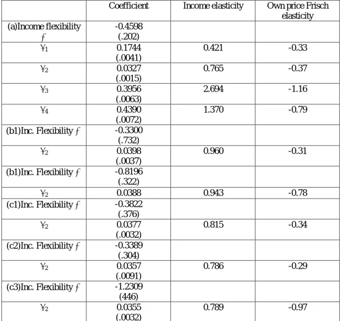
Estimation of the Frisch’s income flexibility Ф =𝝎̌−𝟏 (Polish panels)
Frisch proposed in his 1959 paper to compute directly price elasticities by means of the income elasticity of each good combined with the inverse of the income elasticity of the marginal utility𝜔̌, named by him income flexibility =𝜔̌−1. The method needs only to suppose additive
preferences, either for the direct utility (this is the usual hypothesis we will adopt) or the indirect utility of income and prices. Theil has shown in various studies based on macro time-series (see Theil, 1980, Theil-Clements, 1987, Selvanathan, 1993) that the income flexibility is quite stable across time and countries, and averages at –0.5 (see Selvanathan, p. 308, for the discussion of 322 estimates over 18 countries and 29 years). The direct additivity hypothesis yields the formula for Frisch direct elasticity (under constant marginal utility of income, see for instance Frisch, 1959, Ayanian, 1959 and a direct proof in Deaton, 1974, p. 339-340) :
Eii = -Ei.[wi – (1 – wiEi) 𝜔̌−1]
with wi the budget share for good i and Ei its income elasticity. For goods with a small budget share,
an approximate value gives Eii = Ei/ which corresponds to the Pigou law of proportionality between
income and price elasticities (as the income flexibility is supposed to be constant across the population).
We estimate the income flexibility using a Rotterdam specifiction, as in Theil and Selvanathan studies. The system writes:
wit (Dqit – DQt) = i DQt + (wit+ i)Dp’it (see Selvanathan, pp. 30-31 and Chap. 6)
with Dxt = ln(xt/xt-1), qit real expenditures by unit of consumption for good i in t, DQt = i mwit .Dqit,
wit the average budget share for periods t and (t-1) and Dp’it = Dpit - j (wit +i) Dpjt.
We have estimated this system on the individual data5 of the Polish panel (1987-1990) for four grouped expenditures: 1. food at home and away, 2. alcohol and tobacco, 3. housing and energy, and 4. all other expenditures (financial products excluded).
Table B1. Estimation of a Rotterdam system
Coefficient Income elasticity Own price Frisch
elasticity (a)Income flexibility -0.4598 (.202) 1 0.1744 (.0041) 0.421 -0.33 2 0.0327 (.0015) 0.765 -0.37 3 0.3956 (.0063) 2.694 -1.16 4 0.4390 (.0072) 1.370 -0.79 (b1)Inc. Flexibility -0.3300 (.732) 2 0.0398 (.0037) 0.960 -0.31 (b1)Inc. Flexibility -0.8196 (.322) 2 0.0388 0.943 -0.78 (c1)Inc. Flexibility -0.3822 (.376) 2 0.0377 (.0032) 0.815 -0.34 (c2)Inc. Flexibility -0.3389 (.304) 2 0.0357 (.0091) 0.786 -0.29 (c3)Inc. Flexibility -1.2309 (446) 2 0.0355 (.0032) 0.789 -0.97
Population : Years 1987, 88, 89 of the Polish panel
(a) Whole population with all positive expenditures (1 to 4), N = 2185 (b1) head aged less than 30; (b2) between 35 and 60
(c1) Income per U.C. (Y) less than average income(y) minus half of the standard error () (c2) y-.5 <Y< y+.5
(c3) Y> y+.5
Groups of goods : 1. food at home and away, 2. alcohol and tobacco, 3. housing and energy, and 4. all other expenditures (financial products excluded).
Specification : wit (Dqit – DQt) = i DQt + i (Dpit - Dp’t) with Dp’t = j j Dpjt
i = marginal share = wi + i
The different estimates of the income flexibility are very significant and quite stable for the different populations. The figure for the whole population, - 0.46, is quite similar to the results obtained by Theil-Clements and Selvanathan using macro time-series. This estimate can therefore be used with some confidence to calculate price elasticities under want independency.
An estimation on a French pseudo-panel using the same specification gives an income flexibility equal to -1.18.