HAL Id: hal-00453249
https://hal.archives-ouvertes.fr/hal-00453249
Preprint submitted on 4 Feb 2010
HAL is a multi-disciplinary open access
archive for the deposit and dissemination of
sci-entific research documents, whether they are
pub-lished or not. The documents may come from
L’archive ouverte pluridisciplinaire HAL, est
destinée au dépôt et à la diffusion de documents
scientifiques de niveau recherche, publiés ou non,
émanant des établissements d’enseignement et de
On the distribution of colors in natural images
Antoni Buades, Jose Luis Lisani, Jean-Michel Morel
To cite this version:
Antoni Buades, Jose Luis Lisani, Jean-Michel Morel. On the distribution of colors in natural images.
2010. �hal-00453249�
On the distribution of colors in natural images
A. Buades
∗, J.L Lisani
†and J.M. Morel
‡1
Introduction
When analyzing the RGB distribution of colors in natural images we notice that they are organized into spatial structures. This observation is not new, quoting Omer and Werman in [5]: “... when looking at the RGB histogram of real world images, two important facts can clearly be observed; The histogram is very sparse, and it is structured.[...] This is because the colors of almost any given scene create very specific structures in the histogram”. Omer and Werman observed that colors were distributed along elongated clusters and proposed a linear approximation to model these structures (the color lines).
The use of a linear model for the distribution of colors agrees with the com-mon assumption that the scenes are composed of lambertian objects, for which the emitted surface color depends on the intensity of the illuminant, the re-flectance coefficient and the relative orientation of the surface with respect to the light source (but not with respect to the viewer). In this case the R/G/B ratio at each point of the same object is constant and the colors form a straight line. The non-linearities introduced by the acquisition process (sensor and quan-tization noise, white balance, gamma-correction, etc.) distort these lines and produce the elongated clusters described in [5].
The basic Lambertian model for matte objects can be improved by incorpo-rating the possibility of specular reflections. Klinker, Shafer and Kanade ([3]) introduced the dichromatic reflection model to account for the distribution of colors of matte objects with highlights under controlled illumination conditions. Both the color of the matte object and the highlight are modeled by straight lines that intersect at some point: “The combined spectral cluster of matte and highlight points looks like a skewed T.”. After the acquisition process these lines are distorted but they still conserve their 1D structure.
So far it seems that the linear model is good enough to account for the distribution of colors in natural images. But, is this true in general? As already pointed out in [3]: “A color cluster from an object in an unconstrained scene will generally not be a skewed T composed of linear subclusters because the
∗MAP5, CNRS - Universit´e Paris Descartes, Paris, France. †Dpt Matematiques i Informatica, Universitat Illes Balears, Spain
‡Centre de Math´ematiques et de Leurs Applications, ´Ecole Normale Sup´erieure de Cachan,
illumination color may vary on different parts on the object surface, and the reflection properties of the object may also change, due to illumination changes and to pigment variations in the material body.”. Moreover: “... we need to consider objects with very rough surfaces such that every pixel in the image area has both a significant body and a surface reflection component. The color cluster may then fill out the entire dichromatic plane.” This last sentence suggests that a planar (or 2D) model might be better than the linear model in some cases.
Another hint on the usefulness of a 2D model for the distribution of colors in natural images comes from the work of Chapeau-Blondeau et al. [1], who analized the fractal structure of the three-dimensional color histogram of RGB images. They showed that the fractal dimension of such histograms for several natural images was in the range [1.3, 2.3], which suggests that, in some images, colors are better described by a 2D manifold than by a 1D curve.
Following this line of thought we analyze the distribution of colors of several natural images and discuss the validity of both 1D and 2D models. We propose a dimension reduction algorithm that reveals the underlying 1D or 2D structure of the color clusters and we conclude that, in general, the 2D model fits better the observed distributions.
The paper is organized as follows ...
2
Color representation for dimensionality
anal-ysis
Throughout this paper color is represented in RGB space. We shall call RGB cube the three dimensional representation of colors in RGB space, which is different from the RGB histogram used by other authors (e.g. [5]). Each point will be plotted with the color itself, instead of with a value representing the number of pixels in the image having this color value.
It can be objected that the use of RGB coordinates is arbitrary since many other representations are possible (HSI, La*b*, YUV, etc., to name just a few) some of them presenting interesting properties such as perceptual uniformity. It is however important to remark that the dimensionality of the color clouds (that is, their 1D or 2D character) is independent from this representation. The linear or non-linear conversion formulas between color spaces modify the shape of the color distributions, but not their inherent dimensionality. Since any color space would fit our purposes we chose RGB because it is directly available for most digital images and no color conversion formulas are needed. Moreover, the rest of color spaces introduce strong distortions that increase the image noise.
The same argument can be invoked to justify why JPEG compressed images are used to illustrate the paper, instead of using a non-compressed format or even RAW images (free of white balance and gamma correction). Again, the non-linear processing inside the digital camera modifies the shape of the color distribution but not its dimensionality.
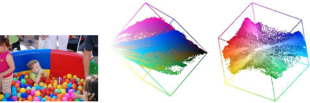
projections of the cube onto the planes defined by the eigenvectors obtained from Principal Components Analysis (PCA) of the color points: the first principal view is given by the first two vectors, the second view by the first and third vectors and the third view by the second and third vectors. Fig. 1 displays an example of a digital image and two views of its RGB cube.
Figure 1: Left, original image and two principal views of its RGB cube.
3
Analysis of the dimensionality of color in
nat-ural images
Fig. 2-center displays a typical distribution of colors in RGB space, correspond-ing to the image patch in Fig. 2-left (patch A). Colors are distributed along an elongated cluster with varying levels of intensity and almost constant hue and saturation. The constancy in hue and saturation is explained by the fact that all the pixels in the patch exhibit a similar color and therefore have similar chromatic components. In fact, if only the intensity component of the colors is modified (as in the shadow region in patch B) the resulting cluster is more elon-gated (it presents a wider range of intensity variation) but hue and saturation remain (almost) unchanged (see Fig. 2-right).
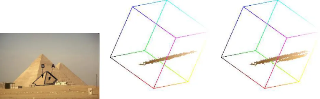
It is interesting to analyze how these 1D clusters combine to form 2D man-ifolds. We display two examples that illustrate how the geometry of the illu-minated objects affects to the distribution of their colors. In the first example (Fig. 3) the RGB distributions of two sides of the same object are compared. When both sides of the object are considered together (patch B) two elongated clusters are visible in RGB space (Fig. 3 right), each one corresponding to a different side of the object. These clusters differ in illumination and saturation, but they exhibit approximately the same hue. As a consequence of the change in orientation the color cluster of the object can be described as a 2D surface (a plane of constant hue) composed by two elongated 1D clusters.
If the change in orientation is smooth, as in the picture of a sphere (patches A and B in Fig. 4) colors are also distributed over a 2D surface of
(approxi-Figure 2: Left, two patches of the same object (grass) under daylight and shadow. Center and right, principal view of the RGB cube of patches A (center) and B (right).
Figure 3: Pyramid example. Left, original image with selected patches. Center and right, principal view of the RGB cube for patches A (center) and B (right). mately) constant hue and high saturation variance, but in this case the colors are uniformly distributed and not organized along 1D subclusters (see Fig. 4).
Figure 4: Ball example. Left, detail of image in Fig. 1-left with selected patches. Center and right, principal views of the RGB cube of patch A (bottom part of the sphere, center) and patch B (full sphere, right).
It is interesting to remark that in this example a highlight was cast on the top of the sphere. In order to avoid the effect of the highlight on the analysis of the color distribution in terms of surface orientation only the bottom of the sphere has been shown in Fig. 4-center. However, when considering the whole sphere (including highlight) we observe how the obtained color distribution (Fig. 4-right) agrees with the dichromatic reflection model proposed by Klinker, Shafer and Kanade in ([3]). According to this model the colors at the highlight can be modelled by a straight line in the direction of the illuminant color. This line is clearly visible in Fig. 4-right. This is an example of a color cluster with non-homogeneus dimensionality where some parts are better modeled by a 2D surface and other parts by a straight line. Anyway, a 2D model can be used for the whole cluster, since 1D ⊂ 2D.
It is important to remark that the changes in geometry that create these 2D structures in RGB space also explain the distribution of colors of “rough” surfaces. As already remarked in [6] most matte objects can not simply be modeled as having a Lambertian surface. A more accurate model [7] describes the surfaces as composed of V-cavities (see Fig. 5), each of them consisting of two planar facets, and each facet assumed to be Lambertian in reflectance. The “roughness” of the surface depends on the distribution of facets slopes. As in the pyramid example, the colors of each facet of the surface are distributed along 1D clusters, but, since there are so many facets at several different orientations the resulting distribution exhibits a 2D structure.
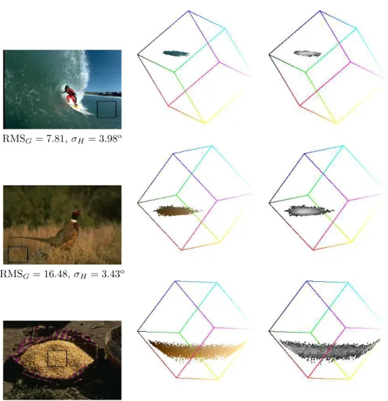
Figure 5: Surface modeled as a collection of V-cavities (source [6]). The following figures (Fig. 6-left) display several patches of different objects with increasing level of “roughness”. The principal view of the RGB cube is dis-played for each one of the patches (Fig. 6-center) together with their densities1 (Fig. 6-right). In can be observed that, as expected, the dimensionality of the color distributions increases with the “roughness” of the patches. Moreover, the
1The density of a color point is defined as the number of neighbors at a fixed distance in
RGB space (we use 5 in all our examples). Color densities are displayed onto the principal views of the RGB cube in such a way that each point in the projection accumulates the density of the RGB points projected onto it. Higher values of cumulated density are displayed as brighter points in this representation.
density of the 2D color clusters is uniform and not composed of distinguishable 1D subclusters.
The “roughness” of the patches is quantified by measuring the root mean square of intensity gradients over the image patch (RMSG)
2
. As an additional information the standard deviation of the hue gradients over the image patch (σH) is also computed to show that all the color clusters lie on a (approximately) constant hue plane.
To end this section we show how the interaction between colors affects the dimensionality of the color distributions. Along edges and blurred regions each pixel combines colors from different objects. This can be observed in the two examples in Fig. 8 and 9.
Fig. 8-top-left displays an image patch containing two objects of different color. The patch is an extract of the image in Fig. 7. In order to show how the colors of both objects interact, we have removed the pixels whose hue has a high gradient value (in practice we use |∇H| > 3, provided that the saturation value is above 10). These pixels correspond to the boundary between both objects (see Fig. 8-top-center). The removed pixels are shown in Fig. 8-top-right. The RGB distributions of these images are displayed in the bottom row of Fig. 8.
We observe that the image of pixels with a low gradient of hue displays the kind of color clusters described in previous examples, corresponding to indi-vidual objects of uniform color. However, the RGB values of the pixels in the boundary between the objects are a mixture of both colors and form a surface that extends between the two original elongated clusters. The same effect is observed when analyzing the interaction between three or more colors (Fig. 9). As the number of colors in the scene increases the structures in RGB space become more and more complex, as can be observed in Fig. 1.
These structures, resulting from the interaction of several colors in the im-ages, can no longer be modeled as simple 1D clusters and the use of a 2D model becomes unavoidable.
4
Quantifying the dimensionality of a color
clus-ter
In the previous section the 1D or 2D character (dimensionality) of a color dis-tribution have been assessed by visual inspection of its representation on RGB space. In this section we propose two methods to quantify this dimensionality.
2The gradient at pixel (i, j) of the intensity image I is defined as ~G = (Gx, Gy), where
Gx= ∂I∂x and Gy= ∂y∂I, which are computed by standard finite differences over four pixels.
The root mean square of the gradient magnitude is RMSG = p|G|2/N , where N is the
RMSG = 7.81, σH= 3.98 o
RMSG= 16.48, σH = 3.43o
RMSG= 61.49, σH = 4.96o
Figure 6: Left: examples of textured image patches. For each patch RMSG assess its “roughness” and σH measures the dispersion of hue values within the color cluster. Center: corresponding principal view of the RGB cube for each image. Observe how the 2D character of the color clusters becomes more obvious as the “roughness” of the patches increases. Right: color densities.
4.1
Fractal dimension
The dimension D of a fractal structure [4] is a statistical quantity that measures how completely the fractal fills the space. The fractal dimension extends the classical concept of dimension in Euclidean space and permits fractal values of
Figure 7: Original image and the selected patches for the study of color inter-action
Figure 8: Top row: left, original patch A (from Fig. 7), low hue gradient pixels (center) and high hue gradient pixels (right). Bottom row: corresponding principal view of the RGB cube for each image.
D. If a set of points in 3D space (e.g. the color points in RGB space) are uniformly distributed along a line or curve then D = 1, if they are distributed over a plane or surface D = 2 and if they are distributed over the whole 3D space D = 3. Fractional values of D account for intermediate distributions.
The fractal dimension may be computed with the method described in [1] by computing the average number of neighbors M (r) within a distance r of a point in RGB space. The slope of the straight line fitting the values of the log-log plot of M (r) versus r gives an approximation of D.
The obtained value of D depends on the size of the image and on the set of r values used for computing M (r). If r is small D tends to 3 since at finer scales all the color distributions are three-dimensional, due to the image noise. If r is bigger than the size of the color cluster M (r) will remain constant as r increases, thus decreasing the value of the estimated D. Moreover, bigger images may produce bigger color clusters, with higher dimension.
Figure 9: Top row: left, original patch B (from Fig. 7), low hue gradient pixels (center) and high hue gradient pixels (right). Bottom row: corresponding principal view of the RGB cube for each image.
In order to avoid the problems related to the size of the image patches and the set of values of r in the computation of the fractal dimension, in our tests we use always the same set of r values r = {6, 12, 18, 24, 30} and all the image patches contain approximately the same number of pixels. Therefore, the obtained values of D give an accurate relative measure of the fractal dimension of the color clusters.
It must be remarked that the fractal dimension gives a global average of the dimension of a cloud of points. Fractional values between 1 and 2 not only account for the presence of a two dimensional aspect but also include a slight thickness or three dimensional effect. We have observed for example when highlights are present (see Fig. 4-right) that both and well differentiated one and two dimensions can arise in the same color cluster.
4.2
Dimension reduction algorithm
We measure how well a color distribution can be modeled by a 1D or 2D manifold by building such a model and then measuring the difference between the original and the modeled RGB values.
The 1D/2D model of a color distribution is built by using a dimensionality reduction algorithm. It is based on the local analysis of the distribution of RGB points by using PCA (Principal Components Analysis). This method of analysis is not new and was already used by Klinker et al. in [3]. The novelty of the approach is that the information provided by the PCA is used to reduce the dimensionality of the cluster, by projecting the points either to a line or a
plane. The algorithm was proposed by Huo and Chen [2] in the context of high dimension data filtering and it is described next.
LLP algorithm
The main idea behind the algorithm is that colors are locally distributed over 1D or 2D dimensional structures contaminated by an additive zero-mean noise that increases the dimensionality of the color distribution. The goal of the algorithm is to extract the local low-dimensional structures.
foreach RGB color yi, i = 1, 2, . . . , N do
Find the K neighbors whose distance to yiis smaller than a given threshold T . The neighboring colors are denoted ˜y1,y˜2, . . . ,y˜K.
Compute the principal components of the set ˜y1,y˜2, . . . ,y˜K.
Let k (k = 1 or k = 2) be the assumed dimension of the embedded manifold, then project yi into the linear subspace spanned by the first k principal components.
end for
The algorithm can be iterated to obtain a better estimation of the low-dimensional structures. When k = 2 the algorithm reveals the surfaces under-lying the distribution of colors. When k = 1 the result of the algorithm are 1D structures.
The algorithm depends on parameter T , which is used to define a neighbor-hood around each color point. The valued is fixed in all the tests to T = 10. If no color points are found in this neighborhood or the number of found points is too small to perform PCA analysis (a minimum number of 10 different points is requested) then the color point cannot be projected and it retains its initial value.
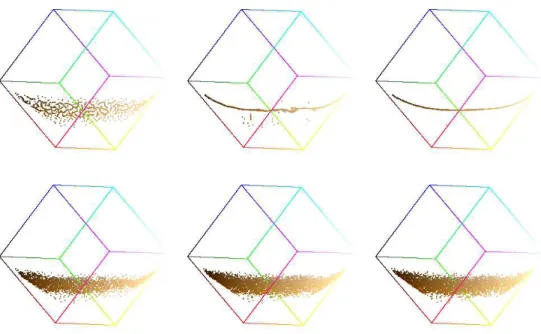
Fig. 10 shows an example of the application of the LLP algorithm to the image patch in Fig. 6 right. The resulting images are visually indistinguishable from the original so only their RGB cubes are shown. The approximation error of each model is measured as the mean square distance in RGB space between the original and the projected color values. ε1D denotes the error of the 1D projection and ε2D of the 2D projection. It can be observed as the 1D model is unable to correctly represent the color distribution, which is mainly 2D. By using larger values of T (see Fig. 11-left) single curves are obtained at the expense of increasing the approximation error. If k = 2 is used for increasing values of T all the results look very similar (see Fig. 11-right), which means that the results are stable with respect to T when using the 2D model. This example illustrates that if the underlying low dimensional structure does not live in the projecting dimension then the projection is unstable and depends extremely on the projection parameter. However this is not the case when we project into the correct dimension. These results reinforce the perception that the 2D model is better suited than the 1D model for representing color distributions.
Figure 10: Two principal views of the RGB cube for image patch in Fig. 6 right. Original (left) and after projection with LLP algorithm with k = 1 (center) and k= 2 (right). The respective projection errors are 9.11 and 2.87.
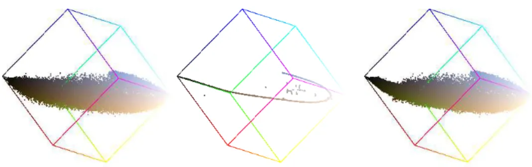
Fig. 12 and 13. In this case the brownish colors of the stones and the greenish tones of the vegetation become gray when projecting to 1D.
Table 14 summarizes the results of computing the fractal dimension and the approximation errors to the 1D and 2D models of the image patches in Fig. 6. We observe a clear correlation between the fractal dimension D, the approx-imation errors ε1D and ε2D and the degree of “roughness” of the image patch. D and ε1D increase with roughness, indicating that the 1D model is unable to account for the color distribution. On the other hand ε2D is always small, since the 2D model is well adapted both for 2D and 1D color distributions. These results agree with the observations of the RGB cube described in the previous section. The 2D error also slightly increases with the fractal dimension since even if the dimension is in between one and two it reflects a slight thickness of the clouds which is removed by the 2D projection. This error also includes the quantization error since distance is computed for 8 bit quantized values.
Finally, let us remark that projection of the colors to a 2D manifold using LLP permits a convenient visualization of color densities: each point in the RGB cube may be represented by a brightness value proportional to the density of the color point. Therefore color densities may be represented in 3D space without the visibility limitations inherent to the representation of 3D point clouds, in which the values of the external points of the cloud hide the values of the internal
Figure 11: Principal views of the RGB cube for image patch in Fig. 6 right. after projection with LLP algorithm with k = 1 and increasing values of T (T = 5, 10, 20 )(top) and k = 2 (bottom). Observe that the result of 2D projection is stable with respect to T .
Figure 12: Left, original image. Result of LLP algorithm (T = 20): center, 1D model; right, 2D model. Observe that in the first case the brownish tones of the stones and the greenish colors of the vegetation become gray. Their corresponding RGB cubes are shown in Fig. 13.
points.
References
[1] Chapeau-Blondeau, F., Chauveau, J., Rousseau, D., and Richard, P. Fractal structure in the color distribution of natural images. Chaos,
Figure 13: Two principals views of the RGB cube for the images in Fig. 12. Original (left) and after applying LLP algorithm with k = 1 (1D model, center) and k = 2 (2D model, right).
Image D RMSG σH ε1D ε2D Sea 1.26 7.81 3.98o 2.78 0.62 Field 1.74 16.48 3.43o 5.50 1.57 Corn 2.19 61.49 4.96o 9.11 2.87
Figure 14: Quantification of the dimensionality of the image patches in Fig. 6 related to their “textureness” and hue constancy.
Solitons and Fractals 42, 1 (2009), 472 – 482.
[2] Huo, X., and Chen, J. Local linear projection (llp). In in Proc. of First Workshop on Genomic Signal Processing and Statistics (GENSIPS (2002). [3] Klinker, G. J., Shafer, S. A., and Kanade, T. A physical approach
to color image understanding. Int. J. Comput. Vision 4, 1 (1990), 7–38. [4] Mandelbrot, B. The fractal geometry of nature. Freeman, 1983.
[5] Omer, I., and Werman, M. Color lines: Image specific color represen-tation. Computer Vision and Pattern Recognition, IEEE Computer Society Conference on 2 (2004), 946–953.
[6] Oren, M., and Nayar, S. K. Generalization of the lambertian model and implications for machine vision. Int. J. Comput. Vision 14, 3 (1995), 227–251.
[7] Torrance, K., and Sparrow, E. Theory for off-specular reflection from rough surfaces. Journal of the Optical Society of America 57 (1967), 1105– 1114.
![Figure 5: Surface modeled as a collection of V-cavities (source [6]).](https://thumb-eu.123doks.com/thumbv2/123doknet/15014431.680441/6.918.368.540.611.761/figure-surface-modeled-collection-v-cavities-source.webp)