Revisiting Horn's problem
20
0
0
Texte intégral
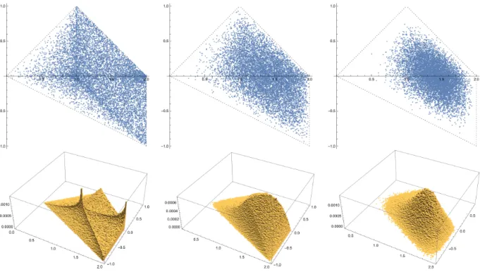
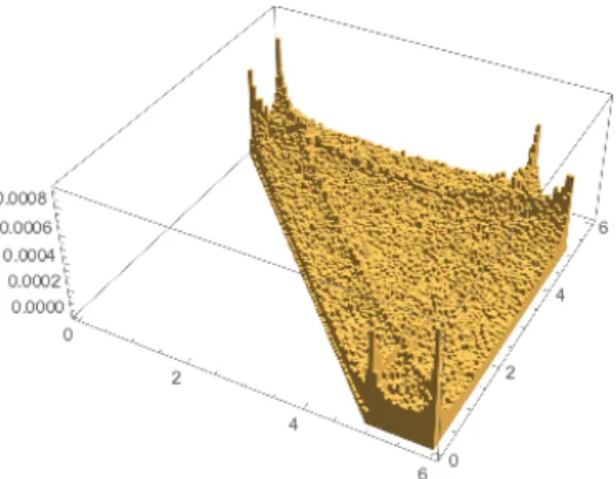
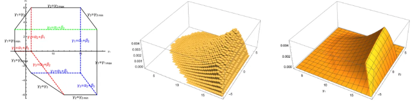
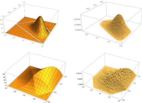
Figure
+5
Documents relatifs