Models and algorithms for metabolic networks: elementary modes and precursor sets

(1)

HAL Id: tel-00850705

https://tel.archives-ouvertes.fr/tel-00850705

Submitted on 8 Aug 2013

HAL is a multi-disciplinary open access archive for the deposit and dissemination of sci-entific research documents, whether they are pub-lished or not. The documents may come from teaching and research institutions in France or abroad, or from public or private research centers.

L’archive ouverte pluridisciplinaire HAL, est destinée au dépôt et à la diffusion de documents scientifiques de niveau recherche, publiés ou non, émanant des établissements d’enseignement et de recherche français ou étrangers, des laboratoires publics ou privés.

Models and algorithms for metabolic networks:

elementary modes and precursor sets

Vicente Acuña

To cite this version:

Vicente Acuña. Models and algorithms for metabolic networks: elementary modes and precursor sets. Algorithme et structure de données [cs.DS]. Université Claude Bernard - Lyon I, 2010. Français. �tel-00850705�

(2)

No _{d’ordre: 218-2008} _{Année 2009}

Thèse

Présentée

devant l’Université Claude Bernard - Lyon 1

pour l’obtention du Diplôme de Doctorat (arrêté du 7 août 2006) et soutenue publiquement le 4 Juin 2010 par

Vicente Acuña

Models and algorithms for metabolic networks:

elementary modes and precursor sets

Directrice de thèse: Marie-France Sagot Co-directeur de thèse: Christian Gautier

Jury: Pierluigi Crescenzi, Rapporteur Khaled Elbassioni, Rapporteur Christian Gautier, Directeur Dominique Perrin, Examinateur Marie-France Sagot, Directrice Alain Viari, Président

(3)

(4)

UNIVERSITÉ CLAUDE BERNARD-LYON 1

Président de l’Université M. le Professeur L. COLLET Vice-Président du Conseil Scientifique M. le Professeur J. F. MORNEX Vice-Président du Conseil d’Administration M. le Professeur G. ANNAT Vice-Président du Conseil des Etudes et M. le Professeur D. SIMON de la Vie Universitaire

Secrétaire Général M. G. GAY

COMPOSANTES SANTÉ

UFR de Médecine Lyon-Est – Claude Bernard Directeur: M. le Professeur J. ETIENNE UFR de Médecine Lyon-Sud – Charles Mérieux Directeur: M. le Professeur F-N. GILLY UFR d’Ontologie Directeur: M. le professeur D. BOURGEOIS Institut des Sciences Pharmaceutiques et

Bi-ologiques

Directeur: M. le Professeur F. LOCHER

Institut des Sciences et Techniques de Réadapta-tion

Directeur: M. le Professeur Y. MATILLON

Département de Formation et Centre de Recherche en Biologie Humaine

Directeur: M. le Professeur P. FARGE

COMPOSANTES SCIENCES ET TECHNOLOGIE

Faculté des Sciences et Technologies Directeur: M. le Professeur F. GIERES UFR Sciences et Techniques des Activités

Physiques et Sportives

Directeur: M. C. Collignon

Observatoire de Lyon Directeur: M. B. Guiderdoni Institut des Sciences et des Techniques de

l’Ingénieur de Lyon

Directeur: M. le Professeur J. LIETO

Institut Universitaire de Technologie A Directeur: M. le Professeur C. COULET Institut Universitaire de Technologie B Directeur: M. le Professeur R. LAMARTINE Institut de Science Financière et d’Assurances Directeur: M. le Professeur J-C. AUGROS

(5)

(6)

Abstract

In this PhD, we present some algorithms and complexity results for two general prob-lems that arise in the analysis of a metabolic network: the search for elementary modes of a network and the search for minimal precursors sets.

Elementary modes is a common tool in the study of the cellular characteristic of a metabolic network. An elementary mode can be seen as a minimal set of reactions that can work in steady state independently of the rest of the network. It has there-fore served as a mathematical model for the possible metabolic pathways of a cell. Their computation is not trivial and poses computational challenges. We show that some problems, like checking consistency of a network, finding one elementary mode or checking that a set of reactions constitutes a cut are easy problems, giving polynomial algorithms based on LP formulations. We also prove the hardness of central problems like finding a minimum size elementary mode, finding an elementary mode containing two given reactions, counting the number of elementary modes or finding a minimum reaction cut. On the enumeration problem, we show that enumerating all reactions containing one given reaction cannot be done in polynomial total time unless P=NP. This result provides some idea about the complexity of enumerating all the elementary modes.

The search for precursor sets is motivated by discovering which external metabolites are sufficient to allow the production of a given set of target metabolites. In contrast with previous proposals, we present a new approach which is the first to formally consider the use of cycles in the way to produce the target. We present a polynomial algorithm to decide whether a set is a precursor set of a given target. We also show that, given a target set, finding a minimal precursor set is easy but finding a precursor set of minimum size is NP-hard. We further show that finding a solution with minimum size internal supply is NP-hard. We give a simple characterisation of precursors sets by the existence of hyperpaths between the solutions and the target. If we consider the enumeration of all the minimal precursor sets of a given target, we find that this problem cannot be solved in polynomial total time unless P=NP. Despite this result, we present two algorithms that have good performance for medium-size networks.

(7)

(8)

Introduction

The principal aim of this work is a computational study of two problems appearing in the research on metabolism. The model used to address these problems considers the set of all biochemical reactions which can occur in a given organism. The links between those reactions and the compounds (or metabolites) that are used/produced by such reactions constitute the metabolic network of the organism. Modelling the whole set of reactions represents a more general approach in comparison to the research that had been done until now on metabolism. Indeed, traditionally biologists and early computational biologists generally concentrated attention on the the study of only a subset of reactions which are able to perform a given task of the cell. This gave rise to the informally defined concept of metabolic pathways. Despite its great interest, this approach may fail to explain some more complex behaviours, that emerge only when the system is analysed as a whole.

In fact, the metabolic network of an organism defined as its set of reactions and compounds correspond to one level of the complex network of interactions that occur in metabolism. Of course, analysing metabolism only at this level without regard to regulation and other types of relations may be insufficient to describe the mechanisms governing the real processes. Indeed, various approaches in what is called systems biology intend to predict the behaviour of metabolism by modelling all kinds of inter-actions occurring in it. There are some reasons however that justify our choice of a simpler model without considering such other interactions:

• Insufficient knowledge of the process and lack of data available for other kinds of interactions make difficult to test the accuracy of more complex models.

• A simple model allows a deeper mathematical theory than considering more het-erogeneous classes of relations.

(13)

12 Introduction

depend on the biological question posed.

• The problems and solutions proposed can be considered as stepping stones in more general and ambitious analysis that integrates other kinds of data.

Considering thus the metabolic network of an organism as a set of reactions and metabolites, we focused our attention on two problems defined on such set:

• the search for elementary modes that correspond to minimal sets of reactions which can work together in steady state independently of the rest of the reactions; and

• the search for precursors sets, which are sets of external source compounds whose presence allows the organism to produce a given target metabolite.

The first concept is commonly used in the analysis of metabolism and has indeed been proposed as a formal definition of metabolic pathway. Several algorithms to enumerate elementary modes could be found in the literature but despite the popularity of the problem, no systematic analysis of its complexity had been done until now. For the second problem, we introduce a new approach which is the first that formally considers cycles in the production of the target compounds by the precursor sets. We then give some useful alternative mathematical characterisations and we analyse the time complexity of finding and enumerating precursor sets.

Analysing the time complexity of these problems gives us a notion about the lim-itations of the algorithms we can aspire to obtain. This serves as a guide on how to continue approaching the problem. For instance, we can know if there is some “hope” of having considerably faster algorithms which find exact solutions or at least a good approximation of them. Or if exact or good solutions were provably hard to find, this would give a good justification to try the use of heuristics.

We show that some of the problems are easy to solve, providing in such cases a polynomial algorithm. Despite the simplicity of the models used, we show that some basic questions are already computationally hard to solve, meaning that finding exact solutions can only be done for small networks under currently believed complexity assumptions. We also show that despite this hardness, in some cases the theoretically slow algorithms run in a reasonable time for real metabolic networks.

We briefly introduce below the two topics covered in this work, including their biological motivation and a summary of our contributions.

(14)

Introduction 13

Finding and enumerating elementary modes

Studying the dynamics of metabolic networks is usually performed using models based on differential equations whereas structural analyses are mainly based on graph-related formalisms or, as far as metabolism is concerned, on a constraint-based modelling. The latter term is commonly employed in the bioinformatics community following two papers by Palsson (Palsson, 2000; Covert et Palsson, 2003). In the constraint-based framework, the network may still be modelled as an edge-labelled hypergraph, but several types of constraints (stoichiometric, thermodynamic and in some cases regulatory) are added to restrict the possible fluxes through the network. The choice of a particular model heavily depends on the type of question one wishes to address (structural or dynamic) but also on the type of data that is available (qualitative or quantitative). Another type of criterion that may be taken into account is the computational cost of a given analysis, and therefore its scalability to large datasets (such as genome-scale metabolic networks).

In a constraint-based approach, only admissible flux distributions are of interest. An admissible flux distribution corresponds to a set of reactions, which, when taken together in given proportions, perform the transformation of available substrates into removable products with the special property that all intermediate compounds are bal-anced (steady-state assumption) and irreversible reactions are taken in the appropriate direction (thermodynamic constraint). Such an admissible flux distribution is called a mode.

Even though each mode is potentially interesting, not all of them are generally considered. Classically, two major sub-problems have been introduced. The first one is known as flux balance analysis. It consists in searching for a mode that optimises a given objective function. Examples of objective functions include biomass (usually rep-resented as a pseudo-reaction of the network, in general determined from experimental data) or ATP production. This optimisation problem has several applications (

Ed-wards et al.,2001;Fong et Palsson, 2004) and can be solved using linear programming

(LP).

The second sub-problem is the one we discuss in this thesis. In the case where no particular function is to be optimised, all modes are equally interesting. A sensible strategy is then to try to find a set that could generate them all. Such a generating set has been proposed and called the set of elementary modes (Schuster et Hilgetag,

1994), EM for short. Intuitively, an elementary mode is a special mode that has the property of not containing any other mode.

(15)

14 Introduction

Elementary modes have been said to represent a formalised definition of a biological pathway. Indeed, a biological interpretation can be given to such flux vectors: a mode is a set of enzymes that operate together at steady state (Schuster et al., 2000) and a mode is elementary when the removal of one enzyme causes it to fail.

Another concept we study here is closely related to the notion of elementary mode. This is the concept of a reaction cut set, recently introduced inKlamt et Gilles (2004). In order to avoid any confusion with other types of cuts in graphs or hypergraphs that may be found in the literature (see e.g. Seymour, 1977), we explicitly choose here to use the term reaction cut. An elementary mode may be seen as a set of reactions that, when used together, perform a given task while a minimal reaction cut set is a set of reactions one needs to inhibit to prevent a given task, also called target reaction, from being performed. As mentioned in Klamt (2006), the task to be silenced can be a combination of reactions. Reaction cut sets have been operationally defined as corresponding to a set of reactions whose deletion from the network stops each elementary mode that contains the target reaction(s).

Previous Work

Surprisingly few results have been established on the complexity of problems concerning detection, counting and enumeration of elementary modes. InKlamt et Stelling(2002), the authors mainly focus on finding an upper bound on the number of elementary modes.

In fact, as mentioned in Fukuda et Prodon (1996), the complexity of the general problem, that is, given a description of a cone (or polytope) in terms of its facets (inequalities), find a description in terms of (enumerate all) its extreme rays (vertices) as a function of the length of the output (number of rays or vertices), is a long-standing open question in computational geometry.

Summary of the main results

The main contribution of this part of our work is in giving a systematic overview of the complexity of optimisation problems related to modes. We first establish results regarding network consistency (Section4.2). Most consistency problems can be solved in polynomial time (are easy). Most, if not all, of these results have been stated before in the literature. It is in fact easy to formulate these problems as LP-problems, which has the side advantage that computer packages are available to solve them.

(16)

Introduction 15

(Sections4.3 and4.4). We show in particular that finding one elementary mode is easy but that this task becomes hard when an elementary mode containing two specified reactions is sought. We also examine a number of EM related problems and establish their complexity. We emphasize that the easy problems can be solved by existing software.

Other complexity results show that it is not possible to generate, in polynomial total time, all elementary modes that pass through a given reaction unless P=NP. This result can have biotechnological relevance. Indeed, by knocking-out enzymes and analysing the effect this has on metabolic behaviour, one can identify whether and where a metabolic network is robust or fragile, and ultimately arrive at a better understanding of cellular phenotypes and of their link with the genotype. Enumerating all elementary modes that pass through a given reaction would thus allow determining all possible steady-state behaviours this reaction enables to block.

We also analyse the computational complexity of problems concerning reaction cuts. We prove that finding a minimum reaction cut set, one that contains a minimum number of reactions, is hard.

Finding and enumerating precursor sets

The metabolic capacities of an organism are directly defined by the set of its possible biochemical reactions. Once the metabolic network of an organism has been defined, the question of how are produced the essential metabolites for the organism arises. In particular, it is important to know which are the metabolites that the organism needs to obtain from its environment to produce those essential metabolites.

One way to answer this question is to manually inspect the metabolic pathways defined as present in the organism. This is determined by comparing the set of reac-tions of a reconstructed metabolic network with the set of reacreac-tions in the reference metabolic pathways contained in metabolic databases such as metacyc from the bio-cyc database collection (Caspi et al.,2006) or kegg (Kanehisa et al.,2006). However, each reference metabolic pathway represents a very small part of the whole network and does not consider what occurs upstream of the pathway, nor whether some alternative organism-specific pathways exist.

With the aim to better understand the relationship between an organism and its environment, we propose a model that allows determining which nutrients an organism requires from its environment in order to produce some metabolic compounds that are

(17)

16 Introduction

essential for its survival.

In particular, the environment could be another living system. This is the case of what is called endosymbiosis where an organism lives within the body or cells of another organism. This concerns mostly bacteria that may inhabit their host intra- or extra-cellularly. Even in the intra-cellular case, a host often accomodates more than one bacterium so that the environment of an endosymbiont is the cell of its host, but also other endosymbionts that may share among them metabolic functions very much like members of a family (should) share chores.

This understanding is in turn important for getting a clearer comprehension of the genotype-phenotype relationship, and ultimately also of the origin of life. Indeed, as is now accepted, one particular endosymbiotic bacterium is the ancestor of an organelle, the mitochondrion, while another evolved into the chloroplast of plants. Understanding how these essential events took place in the course of evolution may be greatly helped by understanding the metabolic dialog between an organism and its living or inanimate environment, what is exchanged between the different partners and how this exchange may evolve through time.

Exploring all the possible ways of producing some metabolic compounds from ex-ternal metabolites may be important also for bioengineering purposes, where the goal is in this case to directly manipulate the environment so that the controlled organism produces what is desired.

Previous work

The capacity to make progress on these questions has been boosted tremendously in the last few years, and this trend will only intensify in the coming decades, by the huge number of sequencing projects, and by our greater ability to now reconstruct whole metabolic networks from such genomic data (seeFrancke et al.,2005, for an overview of such metabolic data reconstruction processes). Surprisingly though, the problem of sys-tematically determining all possible routes from a set of externally acquired metabolites (sources) to the internally produced compounds of interest, henceforth called targets, has not attracted a big literature as is the case for other bioinformatics questions. The issue was first addressed with the purpose to improve the whole network reconstruc-tions by Romero and Karp in the early years of this century (Romero et Karp, 2001), but it is only in 2008 that the first two papers on identifying the sets of metabolites required by an organism to produce some target sets appeared, one by Handorf et al.

(18)

Introduction 17

and our own that was presented at WABI in 2008 (Cottret et al., 2008).

Summary of the main results

An important issue that was not formally treated in the papers of either Romero et al. or Handorf et al. concerned internal cycles in the network. How some of those cycles could be fired off or maintained was not clear, and indeed the problem was addressed in an ad-hoc manner. One of the main contributions of our work is to mathematically address this problem considering cyclic production of some metabolites, which can have also biological sense.

We further address various important complexity questions related to the search for these precursor sets. This concerns in particular the complexity of enumerating all the minimal ones, for which we provide a proof that the problem is indeed hard, in fact it cannot be solved in polynomial total time unless P = N P . We however also show an intriguing relationship with the problem of enumerating the minimal precursor cut sets that can be considered dual of this one and, using a previous elegant result of Gurvich and Khachiyan, prove that the two problems taken together can be solved in quasy-polynomial total time.

Despite its theoretical hardness, two algorithms are proposed for enumerating all minimal set of precursor sets of a given target. Both algorithms are based on the enumeration of paths on the hypergraph or hyperpaths backtracking from the target to the source. This way to travel the hypergraph defines the replacement tree of the network, which was just alluded to in Cottret et al. (2008). The first algorithm for-malises the manipulation that was done to this structure avoiding to maintaining in memory more than a branch of it. Moreover, this algorithm performs some important ideas to prune this structure and thus economise on space and on the number of op-erations without loosing any solution. A second algorithm effects some manipulation and transformation directly on the input network to go much further on the number of redundant operations that is saved. Experimental results show that, in comparison with the previous version (Cottret et al., 2008), the gain in space and in time can be dramatic.

Structure of the manuscript

Chapter 1 gives some of basic mathematical concepts used in the model. It includes a very succinct introduction to graphs and hypergraphs which are used all along the

(19)

18 Introduction

manuscript. It also introduces the concept of hitting set which appears recurrently in the problems studied. Finally monotone boolean functions are presented which are also important in some of the theoretical results on complexity.

Chapter 2 is dedicated to introduce some basic concepts of computational com-plexity. This is restricted only to the time complexity, which is the main interest in our work. In particular, we give some definitions to properly measure time complexity when we want to enumerate all the solutions of certain problems and the number of such solutions can be exponential in the size of the instance.

Chapter 3 presents a brief summary of the biological concepts concerning the metabolism of the cell. We also present some ideas to model metabolic networks from whole set of reactions and metabolites. The models presented in this chapter are used to model the two problems presented in this PhD.

Chapter 4 deals with problems related to the search for elementary modes and reaction cuts. We present algorithms and analyse the complexity of finding and enu-merating these minimal sets of reactions, and present a relation between this problem and a fundamental open question in computational geometry.

Chapter 5 presents our new approach to model precursor sets. It gives different characterisations of such sets and shows the relation with hyperpaths. We also define the related concept of precursor cuts. Finally, in this chapter, we present also our results regarding the time complexity of finding and enumerating precursor sets and precursor cuts of a given target.

Chapter 6 presents two methods to enumerate all the precursor sets of a given target. This includes the algorithmic concept of a replacement tree, which is the main structure used to enumerate the solutions. A brief analysis of the performance of such enumeration is presented as well as some extensions to related problems.

(20)

Chapter 1 Some Basic Mathematical Definitions

This chapter presents a concise introduction to the mathematical concepts used in this work. It does not pretend to be an exhaustive introduction to the topics raised but provides instead the minimum necessary definitions to understand the models presented in the following chapters. For a more detailed description and further theory, see the references given in each section.

1.1 Graphs, digraphs and hypergraphs

In this section, we give a short introduction to graph theory and its extension to hypergraphs. For a more extensive theory, see Diestel (2006), Bang-Jensen et Gutin

(21)

20 Chapter 1. Some Basic Mathematical Definitions

1.1.1 Graph and digraph definitions

A graph G is a pair G = (V, E), where V is a finite set and E is a set whose elements are subsets of V of cardinality two, that is, E ⊆ P2(V). The elements of V are called

vertices or nodes, and the elements of E are called edges.

If G = (V, E) is a graph and e = {v1, v2} ∈ E, then we say that v1 and v2 are the

ends of e. The degree of a vertex v is the number of edges having v as an end.

A directed graph or digraph is a a pair D = (V, A) such that V is a finite set and A is a set of ordered pairs of different elements of V, that is, A ⊆ {(u, v) ∈ V × V | u 6= v}. The elements of V are also called vertices, and the ordered pair of vertices in A are called arcs.

If D = (V, A) is a digraph and a = (v1, v2) ∈ A, then we say that a is an arc from

v1 to v2. The vertices v1 and v2 are called, respectively, the tail and the head of a, and

both are called the ends of e. The indegree of a vertex v is the number of arcs having v as head, and the outdegree of v is the number of arcs having v as tail.

1.1.2 Graphical representation and labels

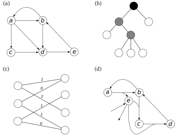
The sets V and E (or A) represent the basic structure that defines G (or D). In general, this topology can be graphically represented by the set of elements in V connected by lines (or arrows for digraphs) between the related pairs (see Figure 1.1 cases (a) and (b)).

Depending on what we are modelling, we can also add some extra information to the vertices or edges (arcs) of G (D). This information is included as functions called labels. For instance, vertices can have colours depending on some classification given to them, and edges/arcs can have weights or costs associated to them.

1.1.3 Walks, paths, cycles and hamiltonian cycles

A walk in a graph G = (V, E) is a sequence of vertices p = (v1, v2, . . . , vk) with k ≥ 1,

such that [vj, vj+1] ∈ E for j = 1, . . . , k − 1. The walk is closed if k > 1 and v1 = vk. A

walk without any repeated nodes in it is called a path. A closed walk with no repeated nodes other than its first and last ones is called a circuit or cycle.

A directed walk in a digraph D = (V, A) is a sequence of vertices p = (v1, v2, . . . , vk)

with k ≥ 1, such that (vj, vj+1) ∈ E for j = 1, . . . , k − 1. A directed walk is closed

(22)

1.1 Graphs, digraphs and hypergraphs 21

directed path. A closed walk with no repeated nodes other than its first and last one is called a directed circuit or directed cycle.

A hamiltonian (directed) cycle is a (directed) cycle that visits each vertex (see Figure 1.1 (a)).

In general, we can also identify paths and cycles by the set of edges (or arcs) connecting the successive vertices they contain.

1.1.4 Adjacency and incidence matrix

For a given order of the elements of V = {v1, . . . , vn} and of E = {e1, . . . , em}, a graph

G = (V, E) can be represented by its adjacency matrix M ∈ Rn×n_{. This matrix is}

such that Mij = 1 if (vi, vj) ∈ E and Mij = 0 otherwise. Hence M is symmetric. We

can define in the same way the adjacency matrix of a digraph, although in this case it is not necessarily symmetric.

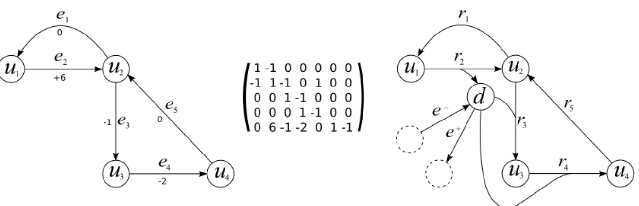
A graph G can also be represented by the incidence matrix I ∈ Rn×m_{. This matrix}

is such that Iij = 1 if vi is an end of ej and Iij = 0 otherwise. In a similar way, we

define the incidence matrix I ∈ Rn×m _{of a digraph D as a matrix such that I}

ij = −1

if vi is the tail of aj, Iij = 1 if vi is the head of aj and Iij = 0 otherwise.

1.1.5 Induced subgraph, bipartite graphs and trees

Given two graphs G = (V, E) and G′ _{= (V}′_{, E}′_{), we say that G}′ _{is a subgraph of G if}

V′ _{⊆ V and E}′ _{⊆ E. We say that G}′ _{is an induced subgraph of G if V}′ _{⊆ V and E}′

contains all the edges of E connecting vertices of V′_.

A graph G = (V, E) is called a bipartite graph if the set of vertices V can be partitioned into two sets U and W , and each edge in E has one end in U and the other end in W (see Figure 1.1 (c)). It is easy to see that a graph is bipartite if and only if it has no cycle of odd length. A matching of a bipartite graph is a subset of edges E ⊆ E such that any pair of edges in E have no ends in common.

Another interesting class of graphs is the class of trees. A graph is connected if for any two nodes in it there is a path between them. A graph T = (V, E) is a tree if it is a connected graph without cycles (see Figure 1.1 (b)). Any vertex of T with degree one is called a leaf. Sometimes we define a vertex of the tree as the root of the tree, indicating that there is a relevant meaning for the paths between this node and the leaves of the tree. In this case, we say that T is rooted. Each vertex other than the root has as parent the next vertex on the path to the root. A child of a vertex u is a

(23)

a

b

c

d

e

1 1 1 0 2 0 (a) (b) (c) (d)

a

b

c

d

e

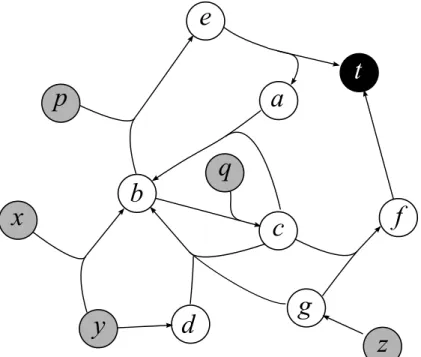
Figure 1.1: Examples of graphs, digraphs and hypergraphs. (a) A digraph con-taining the hamiltonian directed cycle (a, c, d, e, b, a). (b) A tree coloured hav-ing five leaves. If it is rooted at the black vertex, the depth of the tree is three. (c) A bipartite graph where edges are labelled by weights. Edges with weight one forms a matching. (d) A directed hypergraph with hyperarcs (∅, {e}), ({e}, ∅), ({a}, {b, e}), ({b}, {a}), ({b, e}, {c}), ({c, e}, {d}) and ({d}, {b}).

vertex v such that v is the parent of u. Therefore, leaves are the only vertices without children. The depth of the tree is the length of the longest path between a leaf and the root.

1.1.6 Directed hypergraphs

We present a generalisation of the definition of digraphs to the case where arcs, here called hyperarcs, are defined from a set of vertices to another set of vertices.

A directed hypergraph H is a pair H = (C, R), where C is a finite set of vertices and R ⊆ P(C) × P(C) is a set of hyperarcs. Each hyperarc r ∈ R is an ordered pair of disjoint sets r = (T ail(r), Head(r)), both subsets of C (see Figure 1.1 (d) for a graphical representation). For any hyperarc r, one of the sets T ail(r) or Head(r) can be empty but not both. For a given order of the elements of C = {c1, . . . , cn} and of

(24)

1.2 Hitting set 23

R = {r1, . . . , rm}, a hypergraph H = (C, R) can be represented by its incidence matrix

I ∈ Rn×m_{. This matrix is such that I}

ij = −1 if ci ∈ T ail(rj), Iij = 1 if ci ∈ Head(rj)

and Iij = 0 otherwise.

1.2 Hitting set

A concept very often used in this work is that of the hitting set of a collection. Given a finite set U and a collection I = {I1, . . . , In} of subsets of U (that is, Ii ⊆ U for

all i = 1, . . . , n), we say that a set H ⊆ U is a hitting set of I if Ii∩ H 6= ∅ for all

i = 1, . . . , n. In other words if H intersects all the sets in the collection.

The set H is a minimal hitting set of I if H is a hitting set of I and for any H′ _{⊂ H,}

H′ _{is not a hitting set of I (H does not contain other hitting sets of I). There is an}

interesting property of symmetry between the collection I and the collection of all minimal hitting sets of I (see e.g. Berge, 1989).

Property 1.1. Let I = {I1, . . . , In} be a collection of subsets where Ii is not a subset

of Ij for any i 6= j (no set of I is contained in another set of I). Let H be the collection

of all minimal hitting sets of the collection I. Then, I is the collection of all minimal hitting sets of H.

Proof. Let I ∈ I. We show that I is a hitting set of the collection H. Let H be in H. Since H is a hitting set of I, H and I are not disjoint sets. Therefore, I is a hitting set of H.

For the minimality, take I′ _{a subset of I. By hypothesis, for any i ∈ {1, . . . , n} the}

set Ii of the collection is not contained in I′ and therefore Ii\ I′ is not empty. Consider

the set H′ = ∪i∈{1,...,n}Ii \ I′. Clearly H′ is a hitting set of I. Therefore, there exists

H′′ _{⊆ H}′ _{in the collection H. Since I}′ _{does not intersect H}′′_{, we conclude that I}′ _{is not}

a hitting set of H and then I is a minimal hitting set.

Now we show that any minimal hitting set of H belongs to I. Let J be a minimal hitting set of H. Suppose, by contradiction, that J is not in I. In this case J do not contain any Ii (because J and Ii are both minimal hitting sets of H). The set Ii\ J

is not empty for any i ∈ {1, . . . , n}. The set H′ _{= ∪}

i∈{1,...,n}Ii\ J is a hitting set of I.

Therefore, there exists H′′ _{⊆ H}′ _{in the collection H. Since J does not intersect H}′′_{, we}

conclude that J is not a hitting set of H which is a contradiction. We conclude that J is a set of the collection I.

(25)

1.3 Boolean functions

A Boolean function is a function of the form f : {0, 1}k_{→ {0, 1}, where k is a positive}

integer called the arity of f . For example, the function f1 : {0, 1}3 → {0, 1} defined by

f1(x) = x1(1 − x2) + x2x3 is Boolean. Alternatively, the set {0, 1} is also represented

by the set {false, true}.

A propositional formula or Boolean expression in k Boolean variables is a well-formed expression that uses: variables x1, . . . , xk, conjunctions (represented by and or

∧), disjunctions (represented by or or ∨) and negations (represented by not or ¬) and parentheses. For instance, the following are Boolean expressions:

(i) (x1∧ ¬x2) ∨ (x2∧ x3)

(ii) (x1∨ x2) ∧ (x1∨ x3) ∧ (¬x2∨ x3)

(iii) ¬(¬x1∨ x2) ∨ (x2∧ x3)

Every Boolean function of arity k can be expressed as a propositional formula in k variables (for instance, the Boolean function f1 defined above, can be expressed as

the propositional formula (i)). Two Boolean expressions are logically equivalent if and only if they express the same Boolean function (in the example expressions (i), (ii) and (iii) are all equivalent). We say that a propositional formula is satisfiable if there exists an assignment of true and false values to the variables such that the propositional formula evaluates true. For instance, the expressions (i), (ii) and (iii) are satisfiable for x2 = x3 = true.

Given a propositional formula, we define some of its parts. A literal is either a variable or the negation of a variable. A clause is a disjunction of literals and a term is a conjunction of literals. For instance, expression (iii) contains the clause: ¬x1∨ x2

and the term x2∧ x3.

We say that a propositional formula is in conjunctive normal form (CNF) if it is a conjunction of clauses. An important result states that any Boolean function can be expressed as a logically equivalent CNF (for instance, expression (ii) is a CNF of function f1). We say that a propositional formula is in disjunctive normal form (DNF)

if it is a disjunction of terms. Again, any Boolean function can be expressed as a logically equivalent DNF (for instance, expression (i) is a DNF of function f1).

(26)

1.3 Boolean functions 25

1.3.1 Monotone Boolean functions

We say that a Boolean function f : {0, 1}k _{→ {0, 1} is monotone if for any pair}

x, y ∈ {0, 1}k _{such that x}

i ≤ yi for all i ∈ {1, . . . , k} we have that f (x) ≤ f (y).

For example the function f2(x) : {0, 1}3 → {0, 1} defined by

f2(x) =

(

1 if x1(x1+ x2+ x3) > 1

0 otherwise

is a monotone Boolean function.

A propositional formula is called a ∧, ∨-formula if it does not contain any negation. Any monotone Boolean function can be expressed as a ∧, ∨-formula, that is, it can be expressed using variables, conjunctions, disjunctions and parentheses. For instance, f2

can be expressed by

f2(x) = (x1∧ x2) ∨ (x1∧ x3).

Let f be a monotone Boolean function. A prime implicant of f is a minimal set of variables such that if they are all true then f has to be also true. A prime implicate of f is a minimal set of variables such that if they are all false then f has to be also false. In the example, {x1, x2} and {x1, x3} are the prime implicants of f2; and the

sets {x1} and {x2, x3} are the prime implicates of f2.

Any monotone Boolean function f can be expressed as a CNF where the clauses correspond exactly to the set of prime implicants. Any monotone Boolean function f can also be expressed as a DNF where the terms correspond exactly to the set of prime implicates. In the example, f2 can be expressed in CNF and DNF:

f2(x) = (x1∧ x2) ∨ (x1∧ x3) = x1∧ (x2∨ x3).

Finally, it is easy to see that a prime implicate has to contain at least one variable of each prime implicant. In other words, a prime implicate is a minimal hitting set of the collection of prime implicates. Considering Property 1.1, we have the following relation:

Property 1.2. Given a Boolean function f , the collection of its prime implicants corresponds to the minimal hitting sets of its prime implicates, and vice versa.

(27)

(28)

Chapter 2 Basic Concepts of Time Complexity

Analysis

2.1 Defining a problem

We define a problem as a relation P ⊆ IP× SP, where IP is the set of problem instances

and SP is the set of problem solutions. The set of instances represents the particular

cases of the generic problem. If (x, y) ∈ P, we say that y is a solution of x.

For a given instance x ∈ IP of a problem P, we are interested in finding one or

several solutions of x. We can classify a problem depending on the characteristics of the sets IP and SP and depending on which solutions we want to find.

2.1.1 Decision problems

A decision problem is a problem P such that:

1. SP = {no, yes} (or SP = {0, 1})

2. For each x ∈ IP there exists one and only one y ∈ {no, yes} such that (x, y) ∈ P

That is, in a decision problem we want to determine if a given instance x satisfies some condition. In this case, the set of instances can be partitioned into IP = YP∪ NP

such that x ∈ YP if and only if (x, yes) ∈ P. Therefore, we are interested to know

whether x belongs to the set YP.

We present some examples of decision problems. Some of them are classical exam-ples used in this field and some are important for the complexity analyses presented in the next chapters.

• Hitting Set: Given a set of integers I and a collection of subsets I1, . . . , In,

does there exist a hitting set of I1, . . . , In of size at most k?

• Satisfability (Sat): Given a Boolean expression f , does there exist some assignment to the Boolean variables such that f evaluates true?

• st-Path: Given a digraph D and two vertices s and t, does D contain a directed path from s to t?

(30)

2.1 Defining a problem 29

• Directed Hamiltonian Cycle (DHC): Given a digraph D, does D contain a Hamiltonian cycle, i.e. a directed cycle that visit each vertex of D exactly once?

• Perfect Matching: Given a bipartite graph G = (V, E), does E contain a subset E′ _{of edges such that all vertices of the subgraph G}′ _{= (V, E}′_{) have degree}

one?

2.1.2 Optimisation problems

In some cases, although an instance of a problem can have many solutions, there are some that are better than others. In an optimisation problem P, there is a function m : IP × SP → R which measures, for an instance x ∈ IP the cost or benefit of a

solution y of x. We are interested in finding the “best” solution(s) which minimise or maximise m or at least a good approximation to it.

Some examples of optimisation problems are:

• Minimum Hitting Set (minHS): Given a set of integers I and a collection of subsets I1, . . . , In, find a set H ⊆ I of minimum size, such that Ii∩ H 6= ∅ for all

i = 1, . . . , n.

• Linear Programming (LP): Given matrices A ∈ Rm×n_{, b ∈ R}m _{and c ∈ R}n_,

find a vector x ∈ Rn_{such that it satisfies Ax ≤ b and maximises a linear objective}

function cT_x.

• Travelling Salesman (TSP): Given a complete graph G with distances on its edges, find a Hamiltonian cycle of minimum total distance.

• Vertex Cover: Given a graph G = (V, E), find a set C ⊆ V of minimum size, such that each edge of G is incident to at least one vertex in C.

2.1.3 Enumeration and counting problems

For a given P, we are interested in finding not one but all solutions of a given instance x ∈ IP, that is, we want to enumerate all the solutions y ∈ SP such that (x, y) ∈ P.

Some examples of enumeration problems are:

• All Minimal Hitting Sets (AllHS): Given a set of integers I and a collection of subsets I1, . . . , In, find all minimal sets H ⊆ I, such that Ii∩ H 6= ∅ for all

(31)

• All Prime Implicants: Given a Boolean ∧, ∨-formula f , find all prime impli-cants of f .

• All Negative Directed Cycles: Given a digraph D, with integer weights on its arcs, find all negative cycles of D.

In some cases we are interested in counting the number of solutions of a given instance x. In other words, for a given x ∈ IP, we want to obtain k = |{y ∈ SP | (x, y) ∈

P}|. This is the case of the following example:

• Count Perfect Matchings: Given a bipartite graph G, how many perfect matchings does G contain?

2.2 Analysis of algorithms

We give only an intuitive definition of what is an algorithm. For a rigourous definition, we would need to introduce the concept of a Turing machine. This would be out of the scope of this introduction. We thus just say that an algorithm A for a problem P is a sequence of well-defined instructions such that for any instance x ∈ IP given as input,

it executes a list of basic operations in order to return one or more solutions of x. Given a decision problem P, we say that an algorithm A decides P if for any instance x ∈ IP, A(x) returns yes if and only if x ∈ YP. In other words, A computes correctly

if x satisfies the condition defined by P. Turing showed that there exists some decision problems for which there is no algorithm that can give the correct answer for all the instances of the problem (for example see the halting problem). We say that a decision problem P is decidable if there exists an algorithm that decides P.

Of course, most of the “real problems” that we face are decidable, although this does not mean that the problem will be “easy” to be solved. In general, it is not difficult to find, for a given problem P, an algorithm that finds a desirable solution by checking all possible solutions for the given input. For example, we can solve the problem st-Path by checking all the possible directed walks from s in the digraph until a path to t is found or decide that such path does not exist. However, this method is in general impracticable, since it will take an enormous amount of time, specially when the digraph has a considerable size.

In general, for a given problem, we want to have a good algorithm in the sense that it does not take too much time in finding a desirable solution. However, there are many famous problems for which, despite years of work, the best known algorithms to solve

(32)

2.2 Analysis of algorithms 31

them still take an “exponential amount of time”. This concerns algorithms that for some (or all) possible inputs, need to do an exponential number (in terms of the size of the instance) of basic operations to output the solution. Thus, they are methods that can be used only for very small instances of the problem. A natural question that arises in this case is: does there exist an algorithm that solves P in a polynomial number of steps or is P intrinsically “hard”? Can we classify each problem in terms of its intrinsic “complexity”?

With the aim of giving a coherent theory to try to answer this question, we introduce some basic concepts.

2.2.1 Input size

Since problems can be defined over a very dissimilar variety of data, we suppose that the input and the output of an algorithm are encoded as sequences of bits. In other words, if we define the set {0, 1}∗ _{as the set of all finite sequences of 0’s and 1’s, we}

suppose that IP ⊆ {0, 1}∗ and SP ⊆ {0, 1}∗.

For a given instance x ∈ IP, we define the size of x, denoted by |x|, to be the length

of the sequence x.

We suppose that the way of encoding is reasonable in the sense that it does not introduce an artificially redundant information. In general, we can also suppose that for two different reasonable ways of encoding a problem and for any instance x, the size of both codifications of x are not too different (the length of the sequences are polynomially related).

2.2.2 Worst case analysis

Given an algorithm A for a problem P and an instance x ∈ IP of size |x| = n, we

want to measure, in terms of n, the time that A(x) takes to stop. Of course, this time should depend not only on the size of x but on x itself. A way to be conservative, is to consider the worst case, that is, we consider the maximum time that A takes for all the inputs of size n.

2.2.3 Asymptotic analysis

Clearly, the real running time of an algorithm depends on the technology of the ma-chine. Therefore, if we want to have a measure independent of the machine, we should avoid to consider the time used in executing each basic operation. We can do this

(33)

by defining a class of functions that expresses the time asymptotically in terms of the input, independent of the technological characteristics of the machine.

Let A be an algorithm whose running time, in the worst case, is tA(n) (where n is

the size of the input). Let g : N → N be a function. We say that the running time of A is O(g(n)), if there exist constants c and n0 such that, for all n ≥ n0

tA(n) ≤ cg(n).

2.3 Complexity classes of decision problems

2.3.1 The class P

Let P be a decision problem. We say that P belongs to the complexity class P, if P can be decided in polynomial time. In other words, there exists an algorithm A such that P is decided by A and the running time of A is O(nk_{) for some constant k ∈ N.}

Basically to show that a problem is in P, we just need to find a polynomial algorithm which solves it. For example, the problems st-Path and Perfect Matching are known to be in P since there are polynomial algorithms that solve them.

2.3.2 The class Np

There are many important problems for which we do not know whether they belong to P. Can we define a class of decision problems such that we could still have a hope that they belong to P? In effect, most of the problems that we do not know whether they belong to P have at least the property to be easy to check. This means that given an instance x of P such that x ∈ YP and a mathematical object c called certificate of

x, we can verify in polynomial time that x ∈ YP. For instance, consider the problem

Directed Hamiltonian Cycle (DHC). We can easily check that a digraph has a Hamiltonian cycle by showing as certificate c the set of arcs that forms the cycle. Indeed, we can easily verify that c effectively corresponds to a Hamiltonian cycle.

Problems that, given a certificate, are easily checkable form the class Np. Formally, a problem P belongs to the complexity class Np, if there exists a polynomial time algorithm A (the verifier) such that:

• For each instance x ∈ YP, there exists a certificate c(x) (of polynomial size with

(34)

2.3 Complexity classes of decision problems 33

• For each instance x ∈ NP, we have A(x, c) = 0 for any certificate c.

Clearly, any problem in P is also in Np since a verifier is just an algorithm that solves the problem without need to use the certificate. Hence P ⊆ Np.

Apart from DHC and the P problems st-Path and Perfect Matching, other examples of problems in Np are Hitting Set and Sat. All of them are easily checkable by an appropriate certificate.

Note that we said that P ⊆ Np and not P ⊂ Np. Indeed, we cannot discard the possibility that the two sets are equal since there is no proof that there exists a problem in Np which cannot be solved in polynomial time.

2.3.3 Reducibility among problems

A very useful idea when we analyse the complexity of problems, is the reducibility among them. Let P1 and P2 be two decision problems with IP1 and IP2 the respective sets of instances. We say that P1 is reducible to P2 if there is a way to transform

(reduce) any instance x of P1 to an instance R(x) of P2 such that x ∈ YP1 if and only if R(x) ∈ YP2.

This concept is applied to show that, if R is an algorithm that reduces in polynomial time any instance of P1 to an instance of P2, we have that if P2 is in the class P then

P1 is also in the class P. In effect, since there is an algorithm A that solves P2 in

polynomial time, then we can construct an algorithm A′ _{which solves P}

1 in polynomial

time by applying R and A.

2.3.4 Np

-complete problems

Stephen Cook showed (Cook,1971) that the problem Sat has the interesting property that any other problem in Np is polynomial time reducible to it. Hence, if Sat can be solved in polynomial time, then any other Np problem can be solved in polynomial time. This motivates the following definition: A problem P in the class Np is called Np-complete if any other problem in Np is polynomial time reducible to P.

Note that, given a problem P1 in Np and an Np-complete problem P2, if P2 can

be reduced in polynomial time to P1, then P1 is also Np-complete. Using this fact,

many problems have been shown to be Np-complete. Apart from Sat, the problems Hitting Set and DHC are other examples of Np-complete problems.

Np-complete problems are considered the hardest problems in the class Np. Indeed, if we are able to find a polynomial algorithm that solves one Np-complete problem,

(35)

then all the problems in Np can be solved in polynomial time, that is, N P = P . However, despite many years of research, nobody has found an algorithm that solves any single Np-complete problem in polynomial time.

The interest of this concept is that, if we are studying a problem P such that we are not able to find a polynomial time algorithm that solves it, we can alternatively try to find a polynomial time reduction of one Np-complete problem to P. We can then show that P is a new Np-complete problem and therefore, considering all the unsuccessful work spent through the years, that finding a polynomial algorithm to solve it should be very unlikely.

2.4 Complexity classes of optimisation problems

In an optimisation problem, for a given instance x ∈ IP, the set f (x) of feasible solutions

of x is the set of all possible solutions y of x, that is, f (x) = {y ∈ SP | (x, y) ∈ P}.

As we said before, in an optimisation problem P we have an additional function m : IP × SP → R that indicates the cost (or benefit) of a given solution of x. For a

given instance x ∈ IP, we call optimal solution any solution y that minimises the cost

(maximises the benefit), and optimal value the measure of an optimal solution. We are therefore interested in finding a feasible solution y that is an optimal solution or at least that approximates the value of an optimal one.

2.4.1 The classes Po and Npo

Similar to Np for decision problems whose certificates can be checked in polynomial time, for optimisation problems also we can define the class Npo of problems that satisfy some minimal conditions to be considered tractable. Without giving a formal definition, we can say that Npo consists of all the optimisation problems for which there exists a constant k > 0 such that: the instances x can be recognised in polynomial time, the size of any feasible solution y of x is O(|x|k_{), the cost function can be computed in}

polynomial time, and for any instance x and sequence y of size O(|x|k_{) we can decide}

in polynomial time if (x, y) ∈ P.

As for decision problems, we can define the subclass of optimisation problems that are easy to be solved. Given a problem P in the class Npo, we say that P is in the class Po if there exists a polynomial time algorithm A such that, for any instance x ∈ IP,

(36)

2.4 Complexity classes of optimisation problems 35

Examples of problems in Npo are Minimum Hitting Set, Travelling Sales-man and Linear Programming. In particular, we know that Linear Programing can be solved in polynomial time, hence it is in Po.

2.4.2 Np

-hard optimisation problems

As for decision problems, there are many important Npo problems for which we do not know whether there exists a polynomial algorithm. Moreover, many of them are Np-hard in the sense that if they were in Po, then any decision problem in Np could be solved in polynomial time, that is P = Np. Indeed, it has been proved that Po = Npo if and only if P = Np. Therefore, to find a polynomial algorithm that exactly solves an Np-hard optimisation problem should be extremely difficult if not impossible.

One way to prove that an optimisation problem is Np-hard is to consider the de-cision version of the problem. Indeed, we can transform the question of “given x, find a solution with maximum m(x)” into “given x and k, decide if there exists a feasible solution of x with m(x) greater than k". If the latter problem is Np-complete, then the optimisation problem is clearly Np-hard. Problems Vertex Cover, Minimum Hitting Set and Travelling Salesman are examples of Np-hard optimisation problems.

2.4.3 Approximation algorithms

Despite the difficulty in finding exact solutions, many Np-hard optimisation problems have polynomial algorithms that, although they cannot give an optimal solution, guar-antee a feasible solution close to the optimal one.

Let ¯y be any optimal solution of an optimisation problem P. We say that A is an ε(x)-approximation algorithm for some ε(x) > 0 if and only if

|c(x, A(x)) − c(x, ¯y)|

c(x, ¯y) ≤ ε(x)

for any instance x ∈ IP. The value ε(x) is called the approximation ratio.

This definition gives some measure about the accuracy of an algorithm to approach the optimal solution. For instance, we know that Minimum Hitting Set has an O(log n)-approximation where n is the number of sets.

(37)

2.4.4 The classes Apx and Apx-hard

Some classes of problems have been defined depending on the existence and charac-teristics of the approximation algorithms that can solve them. For instance, Apx is the class of optimisation problems for which there exists an ε-approximation algorithm for some fixed (independent of the input) ε > 0. For example, Vertex Cover has a 2-approximation algorithm, and therefore it is in Apx. Unfortunately, Minimum Hitting Set and Travelling Salesman are not in Apx unless P = Np.

The class Apx-hard corresponds to the problems whose approximability is bounded unless P = Np. In other words, a problem is Apx-hard if, under the assumption that P 6= Np, there is b > 0 such that there is no polynomial ε-approximation algorithm for any ε < b. Of course, Minimum Hitting Set and Travelling Salesman are Apx-hard, but also Vertex Cover is Apx-hard. Indeed, it is not approximable within a factor of 1.3606 unless P = Np.

2.5 Complexity of counting solutions

2.5.1 ♯P and ♯P-complete

Suppose that, for a given instance x of a problem P, we want to count the number of solutions y of x. Again, we restrict the problems to those having some minimum conditions. Therefore, we define ♯P to be the set of counting problems such for any instance x ∈ IP and sequence y ∈ {0, 1}∗, we can decide in polynomial time if (x, y) ∈

P.

The complexity class ♯P contains the counting problems associated with decisions problems in Np: for instance, counting the number of Hamiltonian cycles in a digraph is in ♯P. Since if we can count objects, we can decide the existence of at least one of them, a counting problem in ♯P must be at least as hard as the corresponding decision problem. Like the class Np, also ♯P has complete problems, the hardest problems within the class. Solving any of the ♯P-complete problems in polynomial time would prove that any problem in ♯P can be solved in polynomial time, and therefore that P = Np.

There are some ♯P-complete problems that corresponds to some easy decision prob-lems. For instance, although Perfect Matching is in P, the problem Count Per-fect Matchings is ♯P-complete (Valiant, 1979).

(38)

2.6 Complexity of enumerating all the solutions 37

2.6 Complexity of enumerating all the solutions

Given a problem P, we study the time complexity of enumerating all the solutions of any instance x ∈ IP (we suppose that the number of solutions of any x is finite).

However, we must redefine how we measure the time. Indeed, consider, for example, the problem of enumerating all the Hamiltonian cycles of a graph. Note that, in the worst case, the number of solutions can grow exponentially in terms of the size of the graph (consider, for instance, the complete graph that has (n−1)!₂ Hamiltonian cycles). Then, if we measure the running time of some algorithm A for enumerating all the solutions, although A can find each solution in polynomial time, it will be exponential only because it needs exponential time to print all the solutions. For that reason, it is natural to analyse the complexity of enumeration problems with respect to the size of the input and the output.

Moreover, we can consider how an algorithm A that solves P returns the set of solutions. Algorithm A could have the ability of finding one solution and then of repeating the process to find another one, (in which case we can already have some solutions before the end of the complete process) or it may need to compute the total set of solutions at the same time.

Taking into account these considerations, we can classify an enumeration problem P depending on the existence of efficient algorithms that solve it.

2.6.1 Time delay, incremental time and total time

We define three time complexity classes of enumeration problems that have been pro-posed in Johnson et al.(1988).

• An enumeration problem can be solved with polynomial delay if given a set of elements already enumerated, the time needed for generating another element or asserting that no other element exists can be done within a time bounded by a polynomial function of the input size only. We call this class of problems Pd.

• An enumeration problem can be solved in incremental polynomial time if given a set of elements already enumerated, the time needed for generating another element or asserting that no other element exists can be done within a time bounded by a polynomial function of the input size and the number of already enumerated elements. We call this class of problems Pi.

(39)

• An enumeration problem can be solved in polynomial total time if an algorithm exists with running time bounded by a polynomial function of the combined size of the input and the output. We call this class of problems Pt.

It is easy to show that Pd ⊆ Pi ⊆ Pt.

Concerning the enumeration problems introduced, Gurvich et Khachiyan (1999) showed that All Prime Implicants is not in PT unless P=Np. Khachiyan et al.

(2008) showed the same result for the All Negative Directed Cycles enumeration problem. Therefore, these two problems are hard to enumerate.

On the other hand, concerning the All Minimal Hitting Sets enumeration problem,Gurvich et Khachiyan(1999) showed, from a result ofFredman et Khachiyan

(1996), that given a subset of solutions of this problem (that is, minimal hitting sets), we can compute a new solution (or asserting that no other minimal hitting set exists) in time o(k3_{) + k}o(logk) _{with k the combined size of the input and the already enumerated}

solutions. Therefore, All Minimal Hitting Sets can be enumerated in incremental quasi-polynomial time.

(40)

Chapter 3 Metabolic Networks

According to Webster’s Unabridged Dictionary, Metabolism can be defined as “the sum of the physical and chemical processes in an organism by which its material sub-stance is produced, maintained, and destroyed, and by which energy is made available”. In other words, metabolism corresponds to the set of processes and transformations occurring in living organisms in order to maintain life. This comprises, among oth-ers, obtaining energy from the degradation of nutrients (Catabolism) and producing the molecules needed to accomplish specific cellular functions (Anabolism). The set of all biochemical reactions and of all biochemical compounds that are consumed and produced by these reactions forms a network of relations which is called a metabolic network.

Understanding how the metabolic network of an organism performs the needed transformations is not an easy task. Indeed, the set of reactions are also regulated by

(41)

40 Chapter 3. Metabolic Networks

the cell in order to obtain what it needs for each given particular condition. Thus, a metabolic network is just one level of a very complex and heterogeneous network of relations between the set of entities involved in metabolism. We present a brief description of the main entities and levels of interactions, which are defined depending on their general functions and on the nature that each one has.

3.1 Entities involved in metabolism

3.1.1 Biochemical reactions and metabolites

The reactions are the basic transformations of the metabolism. They transform a set of chemical compounds by reordering the atoms that compose them. The set of compounds involved in the reactions are called metabolites. Each reaction transforms a set of metabolites called substrates into another set of metabolites called products of the reaction. For instance, the synthesis of acetolactate transforms the substrate C3H4O3 to produce C5H8O4 and CO2.

Stoichiometry

Sometimes we need to consider not only which compounds are transformed by the re-action but also the amount of each metabolite that is consumed and produced. We call stoichiometry of a reaction the quantitative relations between the metabolites involved. We can add the stoichiometric values to the reaction representation. For instance,

2C3H4O3 → C5H8O4+ CO2

indicates that two molecules of the substrate C3H4O3 are needed to produce a molecule

of C5H8O4 and a molecule of CO2.

Reversibility of reactions

In theory, all reactions can occur in both directions but many of them are considered irreversible when the transformation represented by the reaction happens exclusively or preferentially in only one direction. If a reaction can occur in both directions, we say that it is reversible and a double arrow (↔) is used to represent it. Depending on the kind of analysis, the two directions of a reversible reaction can be considered

Models and algorithms for metabolic networks: elementary modes and precursor sets

HAL Id: tel-00850705

https://tel.archives-ouvertes.fr/tel-00850705

Models and algorithms for metabolic networks:

elementary modes and precursor sets

Vicente Acuña

To cite this version:

Vicente Acuña

Models and algorithms for metabolic networks:

elementary modes and precursor sets

UNIVERSITÉ CLAUDE BERNARD-LYON 1

COMPOSANTES SANTÉ

COMPOSANTES SCIENCES ET TECHNOLOGIE

Abstract

Contents

Introduction

Finding and enumerating elementary modes

Finding and enumerating precursor sets

Structure of the manuscript

Chapter 1

Some Basic Mathematical Definitions

Contents

1.1

Graphs, digraphs and hypergraphs

1.1.1

Graph and digraph definitions

1.1.2

Graphical representation and labels

1.1.3

Walks, paths, cycles and hamiltonian cycles

1.1.4

Adjacency and incidence matrix

1.1.5

Induced subgraph, bipartite graphs and trees

a

b

c

d

e

a

b

c

d

e

1.1.6

Directed hypergraphs

1.2

Hitting set

1.3

Boolean functions

1.3.1

Monotone Boolean functions

Chapter 2

Basic Concepts of Time Complexity

Analysis

Contents

2.1

Defining a problem

2.1.1

Decision problems

2.1.2

Optimisation problems

2.1.3

Enumeration and counting problems

2.2

Analysis of algorithms

2.2.1

Input size

2.2.2

Worst case analysis

2.2.3

Asymptotic analysis

2.3

Complexity classes of decision problems

2.3.1

The class P

2.3.2

The class Np

2.3.3

Reducibility among problems