Detecting Novel Associations in Large Data Sets

(1)

Detecting Novel Associations in Large Data Sets

The MIT Faculty has made this article openly available.

Please share

how this access benefits you. Your story matters.

Citation

Reshef, D. N., Y. A. Reshef, H. K. Finucane, S. R. Grossman, G.

McVean, P. J. Turnbaugh, E. S. Lander, M. Mitzenmacher, and P. C.

Sabeti. “Detecting Novel Associations in Large Data Sets.” Science

334, no. 6062 (December 15, 2011): 1518-1524.

As Published

http://dx.doi.org/10.1126/science.1205438

Publisher

American Association for the Advancement of Science (AAAS)

Version

Author's final manuscript

Citable link

http://hdl.handle.net/1721.1/84636

Terms of Use

Creative Commons Attribution-Noncommercial-Share Alike 3.0

(2)

Detecting Novel Associations in Large Datasets

David N. Reshef1,2,3,*,†, Yakir A. Reshef2,4,*,†, Hilary K. Finucane5, Sharon R. Grossman2,6, Gilean McVean3,7, Peter J. Turnbaugh6, Eric S. Lander2,8,9, Michael Mitzenmacher10,‡, and Pardis C. Sabeti2,6,‡

1_{Department of Computer Science, MIT, Cambridge, MA, USA} 2_{Broad Institute of MIT and Harvard, Cambridge, MA, USA} 3_{Department of Statistics, University of Oxford, Oxford, UK}

4_{Department of Mathematics, Harvard College, Cambridge, MA, USA}

5_{Department of Computer Science and Applied Mathematics, Weizmann Institute of Science,} Rehovot, Israel

6_{Center for Systems Biology, Department of Organismic and Evolutionary Biology, Harvard} University, Cambridge, MA, USA

7_{Wellcome Trust Centre for Human Genetics, University of Oxford, Oxford, UK} 8_{Department of Biology, MIT, Cambridge, MA, USA}

9_{Department of Systems Biology, Harvard Medical School, Boston, MA, USA}

10_{School of Engineering and Applied Sciences, Harvard University, Cambridge, MA, USA}

Abstract

Identifying interesting relationships between pairs of variables in large datasets is increasingly important. Here, we present a measure of dependence for two-variable relationships: the maximal information coefficient (MIC). MIC captures a wide range of associations both functional and not, and for functional relationships provides a score that roughly equals the coefficient of

determination (R2) of the data relative to the regression function. MIC belongs to a larger class of maximal information-based nonparametric exploration (MINE) statistics for identifying and classifying relationships. We apply MIC and MINE to datasets in global health, gene expression, major-league baseball, and the human gut microbiota, and identify known and novel relationships.

Imagine a dataset with hundreds of variables, which may contain important, undiscovered relationships. There are tens of thousands of variable pairs—far too many to examine manually. If you do not already know what kinds of relationships to search for, how do you efficiently identify the important ones? Datasets of this size are increasingly common in fields as varied as genomics, physics, political science, and economics, making this question an important and growing challenge (1, 2).

One way to begin exploring a large dataset is to search for pairs of variables that are closely associated. To do this, we could calculate some measure of dependence for each pair, rank the pairs by their scores, and examine the top-scoring pairs. For this strategy to work, the

†_{To whom correspondence should be addressed. dnreshef@mit.edu (D.N.R.), yreshef@post.harvard.edu (Y.A.R.).}

*These authors contributed equally to this work. ‡These authors contributed equally to this work.

NIH Public Access

Author Manuscript

Science. Author manuscript; available in PMC 2012 June 16.

Published in final edited form as:

Science. 2011 December 16; 334(6062): 1518–1524. doi:10.1126/science.1205438.

NIH-PA Author Manuscript

(3)

statistic we use to measure dependence should have two heuristic properties: generality and equitability.

By generality, we mean that with sufficient sample size the statistic should capture a wide range of interesting associations, not limited to specific function types (such as linear, exponential, or periodic), or even to all functional relationships (3). The latter condition is desirable because not only do relationships take many functional forms, but many important relationships—for example, a superposition of functions—are not well modeled by a function (4-7).

By equitability, we mean that the statistic should give similar scores to equally noisy relationships of different types. For example, we do not want noisy linear relationships to drive strong sinusoidal relationships from the top of the list. Equitability is difficult to formalize for associations in general but has a clear interpretation in the basic case of functional relationships: an equitable statistic should give similar scores to functional relationships with similar R2 values (given sufficient sample size).

In this paper, we describe an exploratory data analysis tool, the maximal information coefficient (MIC), that satisfies these two heuristic properties. We establish MIC's generality through proofs, show its equitability on functional relationships through simulations, and observe that this translates into intuitively equitable behavior on more general associations. Furthermore, we illustrate that MIC gives rise to a larger family of statistics, which we refer to as MINE, or maximal information-based nonparametric exploration. MINE statistics can be used not only to identify interesting associations, but also to characterize them according to properties such as non-linearity and monotonicity. We demonstrate the application of MIC and MINE to datasets in health, baseball, genomics, and the human microbiota.

The Maximal Information Coefficient (MIC)

Intuitively, MIC is based on the idea that if a relationship exists between two variables, then a grid can be drawn on the scatterplot of the two variables that partitions the data to

encapsulate that relationship. Thus, to calculate the MIC of a set of two-variable data we explore all grids up to a maximal grid resolution, dependent on the sample size (Fig. 1A), computing for every pair of integers (x,y) the largest possible mutual information achievable by any x-by-y grid applied to the data. We then normalize these mutual information values to ensure a fair comparison between grids of different dimensions, and to obtain modified values between zero and one. We define the characteristic matrix M = (mx,y), where mx,y is

the highest normalized mutual information achieved by any x-by-y grid, and the statistic MIC to be the maximum value in M. (Fig. 1B,C).

More formally, for a grid G, let IG denote the mutual information of the probability

distribution induced on the boxes of G, where the probability of a box is proportional to the number of data points falling inside the box. The (x,y)-th entry mx,y of the characteristic

matrix equals max{IG}/log min{x,y}, where the maximum is taken over all x-by-y grids G.

MIC is the maximum of mx,y over ordered pairs (x,y) such that xy < B, where B is a function

of sample size; we usually set B = n0.6 (see Section 2.2.1, SOM).

Every entry of M falls between zero and one, and so MIC does as well. MIC is also symmetric (i.e. MIC(X, Y) = MIC(Y, X)) due to the symmetry of mutual information, and because IG depends only on the rank order of the data, MIC is invariant under

order-preserving transformations of the axes. Importantly, although mutual information is used to quantify the performance of each grid, MIC is not an estimate of mutual information (Section 2, SOM).

NIH-PA Author Manuscript

(4)

To calculate M, we would ideally optimize over all possible grids. For computational efficiency, we instead use a dynamic programming algorithm that optimizes over a subset of the possible grids and appears to approximate well the true value of MIC in practice (Section 3, SOM).

Main Properties of MIC

We have proven mathematically that MIC is general in the sense described above. Our proofs show that, with probability approaching 1 as sample size grows, (i) MIC assigns a perfect score of 1 to all never-constant noiseless functional relationships, (ii) MIC assigns scores that tend to 1 for a larger class of noiseless relationships (including superpositions of noiseless functional relationships), and (iii) MIC assigns a score of 0 to statistically independent variables.

Specifically, we have proven that for a pair of random variables X and Y, (i) if Y is a function of X that is not constant on any open interval, then data drawn from (X,Y) will receive an MIC tending to 1 with probability one as sample size grows; (ii) if the support of (X,Y) is described by a finite union of differentiable curves of the form c(t) = (x(t),y(t)) for t in [0,1], then data drawn from (X,Y) will receive an MIC tending to 1 with probability one as sample size grows, provided that dx/dt and dy/dt are each zero on finitely many points; (iii) the MIC of data drawn from (X,Y) converges to zero in probability as sample size grows if and only if

X and Y are statistically independent. We have also proven that the MIC of a noisy

functional relationship is bounded from below by a function of its R2. (For proofs, see SOM.)

We tested MIC's equitability through simulations. These simulations confirm the

mathematical result that noiseless functional relationships (i.e. R2 = 1.0) receive MIC scores of 1.0 (Fig. 2A). They also show that, for a large collection of test functions with varied sample sizes, noise levels, and noise models, MIC roughly equals the coefficient of determination R2 relative to each respective noiseless function. This makes it easy to interpret and compare scores across various function types (Fig. 2B, S4). For instance, at reasonable sample sizes, a sinusoidal relationship with a noise level of R2 = 0.80 and a linear relationship with the same R2 value receive nearly the same MIC score. For a wide range of associations that are not well modeled by a function, we also show that MIC scores degrade in an intuitive manner as noise is added (Fig. 2G, Figs. S5-6).

Comparisons to Other Methods

We compared MIC to a wide range of methods – including methods formulated around the axiomatic framework for measures of dependence developed by Rényi (8), other state-of-the-art measures of dependence, and several nonparametric curve estimation techniques that can be used to score pairs of variables based on how well they fit the estimated curve. Methods such as splines (1) and regression estimators (1, 9, 10) tend to be equitable across functional relationships (11), but are not general: they fail to find many simple and

important types of relationships that are not functional. (Figs. S5 and S6 depict examples of relationships of this type from existing literature, and compare these methods to MIC on such relationships.) Although these methods are not intended to provide generality, the failure to assign high scores in such cases makes them unsuitable for identifying all potentially interesting relationships in a dataset.

Other methods such as mutual information estimators (12-14), maximal correlation (8, 15), principal curve-based methods (16-19)(20), distance correlation (21), and the Spearman rank correlation coefficient all detect broader classes of relationships. However, they are not

NIH-PA Author Manuscript

(5)

equitable even in the basic case of functional relationships: they show a strong preference for some types of functions, even at identical noise levels (Fig. 2A,C-F). For example, at a sample size of 250, the Kraskov et al. mutual information estimator (14) assigns a score of 3.65 to a noiseless line but only 0.59 to a noiseless sinusoid, and it gives equivalent scores to a very noisy line (R2 = 0.35) and to a much cleaner sinusoid (R2 = 0.80) (Fig. 2D). Again, these results are not surprising—they correctly reflect the properties of mutual information. But this behavior makes these methods less practical for data exploration.

An Expanded Toolkit for Exploration

The basic approach of MIC can be extended to define a broader class of MINE statistics based on both MIC and the characteristic matrix M. These statistics can be used to rapidly characterize relationships that may then be studied with more specialized or computationally intensive techniques.

Some statistics are derived, like MIC, from the spectrum of grid resolutions contained in M. Different relationship types correspond to different characteristic matrices (Fig. 3). For example, just as a characteristic matrix with a high maximum indicates a strong relationship, a symmetric characteristic matrix indicates a monotonic relationship. We can thus detect deviation from monotonicity with the Maximum Asymmetry Score (MAS), defined as the maximum over M of |mx,y − my,x|. MAS is useful, for example, for detecting periodic

relationships with unknown frequencies that vary over time, a common occurrence in real data (22). MIC and MAS together detect such relationships more effectively than either Fisher's test (23) or a recent specialized test developed by Ahdesmaki et al. (Figs. S8-9) (24).

Because MIC is general and roughly equal to R2 on functional relationships, we can also define a natural measure of non-linearity by MIC − ρ2_{, where ρ denotes the Pearson}

product-moment correlation coefficient, a measure of linear dependence. The statistic MIC − ρ2_{is near 0 for linear relationships and large for non-linear relationships with high values}

of MIC. As seen in the real-world examples below, it is useful for uncovering novel non-linear relationships.

Similar MINE statistics can be defined to detect properties that we refer to as “complexity” and “closeness to being a function.” We provide formal definitions and a performance summary of these two statistics (Section 2.3, SOM, Table S1). Finally, MINE statistics can also be used in cluster analysis to observe the higher-order structure of datasets (Section 4.9, SOM).

Application of MINE to real datasets

We used MINE to explore four high-dimensional datasets from diverse fields. Three datasets have previously been analyzed and contain many well-understood relationships. These datasets are (i) social, economic, health, and political indicators from the World Health Organization (WHO) and its partners (7, 25); (ii) yeast gene expression profiles from a classic paper reporting genes whose transcript levels vary periodically with the cell cycle (26); and (iii) performance statistics from the 2008 Major League Baseball (MLB) season (27, 28). For our fourth analysis, we applied MINE to a dataset that has not yet been exhaustively analyzed: a set of bacterial abundance levels in the human gut microbiota (29). All relationships discussed in this section are significant at a false discovery rate of 5%; p-values and q-p-values are listed in the SOM.

We explored the WHO dataset (357 variables, 63,546 variable pairs) with MIC, the commonly used Pearson correlation coefficient (ρ), and Kraskov's mutual information

NIH-PA Author Manuscript

(6)

estimator (Fig. 4, Table S9). All three statistics detected many linear relationships. However, mutual information gave low ranks to many non-linear relationships that were highly ranked by MIC (Figs. 4A-B). Two-thirds of the top 150 relationships found by mutual information were strongly linear (|ρ| ≥ 0.97), whereas most of the top 150 relationships found by MIC had |ρ| below this threshold. Further, although equitability is difficult to assess for general associations, the results on some specific relationships suggest that MIC comes closer than mutual information to this goal (Fig. 4I). Using the non-linearity measure MIC − ρ2_{, we}

found several interesting relationships (Figs. 4E-G), many of which are confirmed by existing literature (30-32). For example, we identified a superposition of two functional associations between female obesity and income per person, one from the Pacific Islands, where female obesity is a sign of status, (33) and one from the rest of the world, where weight and status do not appear to be linked in this way (Fig. 4F).

We next explored a yeast gene expression dataset (6,223 genes) that was previously analyzed with a special-purpose statistic developed by Spellman et al. to identify genes whose transcript levels oscillate during the cell cycle (26). Of the genes identified by Spellman et al. and MIC, 70% and 69%, respectively, were also identified in a later study with more time points conducted by Tu et al. (22). However, MIC identified genes at a wider range of frequencies than Spellman et al., and MAS sorted those genes by frequency (Fig. 5). Of the genes identified by MINE as having high frequency (MAS > 75th

percentile), 80% were identified by Spellman et al., while of the low-frequency genes (MAS < 25th percentile) Spellman et al. identified only 20% (Fig. 5B). For example, although both methods found the well-known cell-cycle regulator HTB1 (Fig. 5G) required for chromatin assembly, only MIC detected the heat-shock protein HSP12 (Fig. 5E), which Tu et al. confirmed to be in the top 4% of periodic genes in yeast. HSP12, along with 43% of the genes identified by MINE but not Spellman et al., was also in the top third of statistically significant periodic genes in yeast according to the more sophisticated specialty statistic of Ahdesmaki et al., which was specifically designed for finding periodic relationships without a pre-specified frequency in biological systems (24). Due to MIC's generality and the small size of this dataset (n=24), relatively few of the genes analyzed (5%) had significant MIC scores after multiple testing correction at a false discovery rate of 5%. However, using a less conservative false discovery rate of 15% yielded a larger list of significant genes (16% of all genes analyzed) and this larger list still attained a 68% confirmation rate by Tu et al.. In the MLB dataset (131 variables), MIC and ρ both identified many linear relationships, but interesting differences emerged. On the basis of ρ, the strongest three correlates with player salary are walks, intentional walks, and runs batted in. In contrast, the strongest three associations according to MIC are hits, total bases, and a popular aggregate offensive statistic called Replacement Level Marginal Lineup Value (27)(34) (Fig. S12, Table S12). We leave it to baseball enthusiasts to decide which of these statistics are (or should be!) more strongly tied to salary.

Our analysis of gut microbiota focused on the relationships between prevalence levels of the trillions of bacterial species that colonize the gut of humans and other mammals (35, 36). The dataset consisted of large-scale sequencing of 16S ribosomal RNA from the distal gut microbiota of mice colonized with a human fecal sample (29). After successful colonization, a subset of the mice was shifted from a low-fat/plant-polysaccharide-rich (LF/PP) diet to a high-fat/high-sugar ‘Western’ diet. Our initial analysis identified 9,472 significant relationships (out of 22,414,860) between ‘species’-level groups called operational taxonomic units (OTUs); significantly more of these relationships occurred between OTUs in the same bacterial family than expected by chance (30% vs. 24±0.6%).

NIH-PA Author Manuscript

(7)

Examining the 1,001 top-scoring non-linear relationships (MIC-ρ2>0.2), we observed that a common association type was ‘non-coexistence’: when one species is abundant the other is less abundant than expected by chance, and vice versa (Fig. 6A-B,D). Additionally, we found that 312 of the top 500 non-linear relationships were affected by one or more factors for which data were available (host diet, host sex, identity of human donor, collection method, and location in the gastrointestinal tract; SOM, Section 4.7). Many are non-coexistence relationships that are explained by diet (Fig. 6A, Table S13). These diet-explained non-coexistence relationships occur at a range of taxonomic depths—inter-phylum, inter-family, and intra-family—and form a highly interconnected network of non-linear relationships (Fig. 6E).

The remaining 188 of the 500 highly ranked non-linear relationships were not affected by any of the factors in the dataset, and included many non-coexistence relationships (Table S14, Fig. 6D). These unexplained non-coexistence relationships may suggest interspecies competition and/or additional selective factors that shape gut microbial ecology, and therefore represent promising directions for future study.

Conclusion

Given the ever-growing, technology-driven data stream in today's scientific world, there is an increasing need for tools to make sense of complex datasets in diverse fields. The ability to examine all potentially interesting relationships in a dataset—independent of their functional form—allows tremendous versatility in the search for meaningful insights. On the basis of our tests, MINE is useful for identifying and characterizing structure in data.

Supplementary Material

Refer to Web version on PubMed Central for supplementary material.

Acknowledgments

The authors thank C. Blättler, B. Eidelson, M.D. Finucane, M.M. Finucane, M. Fujihara, T. Gingrich, E. Goldstein, R. Gupta, R. Hahne, T. Jaakkola, N. Laird, M. Lipsitch, S. Manber, G. Nicholls, A. Papageorge, N. Patterson, E. Phelan, J.Rinn, B. Ripley, I. Shylakhter, and R. Tibshirani for their invaluable support and critical discussions throughout; and O. Derby, M. Fitzgerald, S. Hart, M. Huang, E. Karlsson, S. Schaffner, C. Edwards and D. Yamins for assistance. PCS and this work are supported by the Packard Foundation, MM by NSF grant 0915922, HKF by ERC grant no. 239985, SRG by MSTP, and PJT by NIH P50 GM068763. Data and software are available online at http://exploredata.net.

References

1. Hastie, T.; Tibshirani, R.; Friedman, JH. The elements of statistical learning: data mining, inference, and prediction. Springer Verlag; 2009.

2. Science Staff, Challenges and opportunities. Science. 2011; 331:693.

3. By ‘functional relationship’ we mean a distribution (X,Y) in which Y is a function of X, potentially with independent noise added.

4. Caspi A, et al. Influence of life stress on depression: moderation by a polymorphism in the 5-HTT gene. Science. 2003; 301:386. [PubMed: 12869766]

5. Clayton RN, Mayeda TK. Oxygen isotope studies of achondrites. Geochimica et Cosmochimica Acta. 1996; 60:1999.

6. Algeo TJ, Lyons TW. Mo-total organic carbon covariation in modern anoxic marine environments: Implications for analysis of paleoredox and paleohydrographic conditions. Paleoceanography. 2006; 21:1016.

7. World Health Organization Statistical Information Systems. World Health Organization Statistical Information Systems (WHOSIS). 2009. http://www.who.int/whosis/en/

NIH-PA Author Manuscript

(8)

8. Rényi A. On measures of dependence. Acta Mathematica Hungarica. 1959; 10:441. 9. Stone CJ. Consistent nonparametric regression. The annals of statistics. 1977:595.

10. Cleveland WS, Devlin SJ. Locally weighted regression: an approach to regression analysis by local fitting. Journal of the American Statistical Association. 1988; 83:596.

11. For both splines and regression estimators, we used R2 with respect to the estimated spline/ regression function to score relationships.

12. Moon Y, Rajagopalan B, Lall U. Estimation of mutual information using kernel density estimators. Physical Review E. 1995; 52:2318.

13. Darbellay G, Vajda I. Estimation of the information by an adaptive partitioning of the observation space. IEEE Transactions on Information Theory. 1999; 45:1315.

14. Kraskov A, Stögbauer H, Grassberger P. Estimating mutual information. Physical Review E. 2004; 69:66138.

15. Breiman L, Friedman JH. Estimating optimal transformations for multiple regression and correlation. Journal of the American Statistical Association. 1985; 80:580.

16. Hastie T, Stuetzle W. Principal curves. Journal of the American Statistical Association. 1989; 84:502.

17. Tibshirani R. Principal curves revisited. Statistics and Computing. 1992; 2:183.

18. Kégl B, Krzyzak A, Linder T, Zeger K. A polygonal line algorithm for constructing principal curves. Advances in Neural Information Processing Systems. 1999:501.

19. Delicado P, Smrekar M. Measuring non-linear dependence for two random variables distributed along a curve. Statistics and Computing. 2009; 19:255.

20. “Principal curve-based methods” refers to mean-squared error relative to the principal curve, and CorGC, the principal curve-based measure of dependence of Delicado et al

21. Székely G, Rizzo M. Brownian distance covariance. Annals. 2009; 3:1236.

22. Tu B, Kudlicki A, Rowicka M, McKnight S. Logic of the yeast metabolic cycle: temporal compartmentalization of cellular processes. Science. 2005; 310:1152. [PubMed: 16254148] 23. Fisher R. Tests of significance in harmonic analysis. Proceedings of the Royal Society of London.

1929:54.Series A, Containing Papers of a Mathematical and Physical Character

24. Ahdesmäki M, Lähdesmäki H, Pearson R, Huttunen H, Yli-Harja O. Robust detection of periodic time series measured from biological systems. BMC bioinformatics. 2005; 6:117. [PubMed: 15892890]

25. Rosling, H. Gapminder, Indicators in Gapminder World. 2008.

http://www.gapminder.org/gapminder-world/indicators-in-gapminder-world/

26. Spellman P, et al. Comprehensive identification of cell cycle-regulated genes of the yeast Saccharomyces cerevisiae by microarray hybridization. Molecular biology of the cell. 1998; 9:3273. [PubMed: 9843569]

27. Baseball Prospectus Statistics Reports. 2009. http://www.baseballprospectus.com/statistics/ 28. Lahman, S. The Baseball Archive. The Baseball Archive. 2009. http://www.baseball1.com/ 29. Turnbaugh PJ, et al. The effect of diet on the human gut microbiome: a metagenomic analysis in

humanized gnotobiotic mice. Science translational medicine. 2009; 1:6ra14.

30. Chen L, et al. Human resources for health: overcoming the crisis. The Lancet. 2004; 364:1984. 31. Desai S, Alva S. Maternal education and child health: Is there a strong causal relationship?

Demography. 1998; 35:71. [PubMed: 9512911]

32. Gupta S, Verhoeven M. The efficiency of government expenditure: experiences from Africa. Journal of Policy Modeling. 2001; 23:433.

33. Gill, T., et al. Obesity in the Pacific: Too big to ignore. Noumea, New Caledonia: World Health Organization Regional Office for the Western Pacific, Secretariat of the Pacific Community; 2002. 34. RPMLV estimates how many more runs per game a player contributes over a replacement-level

player in an average lineup

35. Turnbaugh PJ, et al. The human microbiome project. Nature. 2007; 449:804. [PubMed: 17943116] 36. Ley RE, et al. Evolution of mammals and their gut microbes. Science. 2008; 320:1647. [PubMed:

18497261]

NIH-PA Author Manuscript

(9)

37. The World Factbook, 2009. Central Intelligence Agency; Washington, DC: 2009.

38. Cover, T.; Thomas, J. Elements of information theory. John Wiley & Sons, Inc.; New York: 2006. 39. Steuer R, Kurths J, Daub C, Weise J, Selbig J. The mutual information: detecting and evaluating

dependencies between variables. Bioinformatics. 2002; 18:231.

40. Theiler J, Galdrikian B, Longtin A, Eubank S, Farmer J. Testing for nonlinearity in time series: the method of surrogate data. Physica D. 1991; 58:77.

41. Benjamini Y, Hochberg Y. Controlling the false discovery rate: a practical and powerful approach to multiple testing. Journal of the Royal Statistical Society. 1995; 57:289.Series B

(Methodological)

42. Devlin B, Roeder K, Wasserman L. False discovery or missed discovery? HEREDITY-LONDON. 2003; 91:537.

43. Noble WS. How does multiple testing correction work? Nature biotechnology. 2009; 27:1135. 44. Benjamini Y, Yekutieli D. The control of the false discovery rate in multiple testing under

dependency. Annals of statistics. 2001:1165. 45. Weingessel MA. Package ‘princurve’. 2009

46. Delicado P, Huerta M. Principal curves of oriented points: theoretical and computational improvements. Computational Statistics. 2003; 18:293.

47. Fruchterman TMJ, Reingold EM. Graph drawing by force-directed placement. Software- Practice and Experience. 1991; 21:1129.

48. Bernstein JT. Traer Physics 3.0. 2009

49. Mitzenmacher, M.; Upfal, E. Probability and computing: Randomized algorithms and probabilistic analysis. Cambridge University Press; New York: 2005.

50. Roulston M. Estimating the errors on measured entropy and mutual information. Physica D: Nonlinear Phenomena. 1999; 125:285.

51. Durrett, R. Probability: theory and examples. Cambridge Univ Pr;

52. Dubhashi, D.; Panconesi, A. Concentration of Measure for the Analysis of Randomized Algorithms. Cambridge University Press; New York: 2009. p. 216

53. Xiang D, Wahba G. A generalized approximate cross validation for smoothing splines with non-Gaussian data. Statistica Sinica. 1996; 6:675.

54. Cleveland WS. Robust locally weighted regression and smoothing scatterplots. Journal of the American Statistical Association. 1979; 74:829.

NIH-PA Author Manuscript

(10)

Figure 1. Computing MIC

(A) For each pair (x,y), the MIC algorithm finds the x-by-y grid with the highest induced mutual information. (B) The algorithm normalizes the mutual information scores and compiles a matrix that stores, for each resolution, the best grid at that resolution and its normalized score. (C) The normalized scores form the characteristic matrix, which can be visualized as a surface; MIC corresponds to the highest point on this surface. In this

example, there are many grids that achieve the highest score. The star in (B) marks a sample grid achieving this score, and the star in (C) marks that grid's corresponding location on the surface.

NIH-PA Author Manuscript

(11)

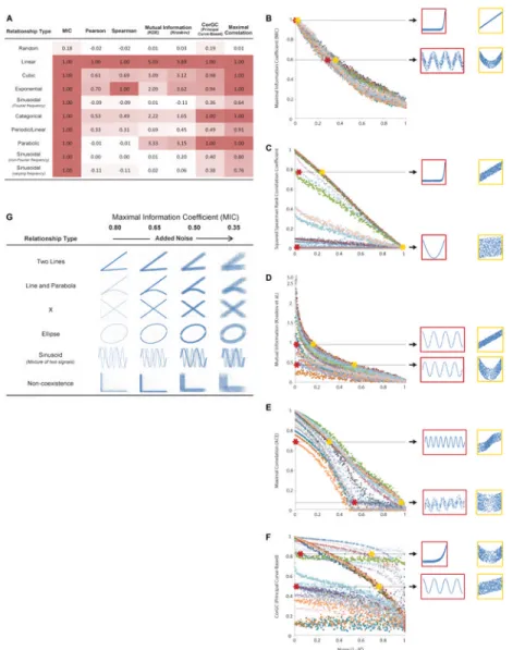
Figure 2. Comparison of MIC to Existing Methods

(A) Scores given to various noiseless functional relationships by several different statistics (8, 12, 14, 19). Maximal scores in each column are accentuated. (B-F) The MIC, Spearman correlation coefficient, mutual information (Kraskov et al. estimator), maximal correlation (via ACE), and the principal curve-based CorGC dependence measure, respectively, of 27 different functional relationships with independent uniform vertical noise added, as the R2 value of the data relative to the noiseless function varies. Each shape/color corresponds to a different combination of function type and sample size. In each plot, pairs of thumbnails show relationships that received identical scores; for data exploration, we would like these pairs to have similar noise levels. For a list of the functions and sample sizes in these graphs as well as versions with other statistics, sample sizes, and noise models, see Figs. S3 and S4. (G) Performance of MIC on associations not well modeled by a function, as noise level varies. For the performance of other statistics, see Figs. S5 and S6.

NIH-PA Author Manuscript

(12)

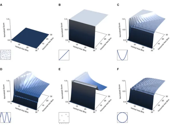
Figure 3. Visualizations of the Characteristic Matrices of Common Relationships

(A-F) Surfaces representing the characteristic matrices of several common relationship types. For each surface, the x-axis represents number of vertical axis bins (rows), the y-axis represents number of horizontal axis bins (columns), and the z-axis represents the

normalized score of the best-performing grid with those dimensions. The inset plots show the relationships used to generate each surface. For surfaces of additional relationships see Fig. S7.

NIH-PA Author Manuscript

(13)

Figure 4. Application of MINE to Global Indicators from the World Health Organization (A) MIC versus ρ for all pairwise relationships in the WHO dataset. (B) Mutual information (Kraskov et al. estimator) versus ρ for the same relationships. High mutual information scores tend to be assigned only to relationships with high ρ, while MIC gives high scores also to relationships that are non-linear. (C-H) Example relationships from (A). (C) Both ρ and MIC yield low scores for uncorrelated variables. (D) Ordinary linear relationships score high under both tests. (E-G) Relationships detected by MIC but not by ρ, because the relationships are non-linear (E,G) or because more than one relationship is present (F). In (F), the linear trendline comprises a set of Pacific island nations in which obesity is culturally valued (33); most other countries follow a parabolic trend (Table S10). (H) A superposition of two relationships that scores high under all three tests, presumably because the majority of points obey one relationship. The less steep minority trend consists of thirteen countries whose economies rely largely on oil (37) (Table S11). The lines of best fit in (D-H) were generated using polynomial regression on each trend. (I) Of these four relationships, the left two appear less noisy than the right two. MIC accordingly assigns higher scores to the two relationships on the left. In contrast, mutual information assigns similar scores to the top two relationships and similar scores to the bottom two relationships.

NIH-PA Author Manuscript

(14)

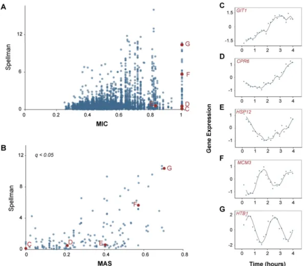
Figure 5. Application of MINE to S cerivisiae Gene Expression Data

(A) MIC versus scores obtained by Spellman et al. for all genes considered (26). Genes with high Spellman scores tend to receive high MIC scores, but some genes undetected by Spellman's analysis also received high MICs. (B) MAS versus Spellman's statistic for genes with significant MICs. Genes with a high Spellman score also tend to have a high MAS score. (C-G) Examples of genes with high MIC and varying MAS (trend-lines are moving averages). MAS sorts the MIC-identified genes by frequency. A higher MAS signifies a shorter wavelength for periodic data, indicating that the genes found by Spellman et al. are those with shorter wavelengths. None of the examples except for (F) and (G) were detected by Spellman's analysis. However, subsequent studies have shown that (C-E) are periodic genes with longer wavelengths (22, 24). More plots of genes detected using MIC and MAS are given in Fig. S11.

NIH-PA Author Manuscript

(15)

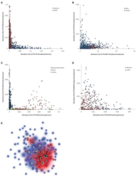
Figure 6. Associations Between Bacterial Species in the Gut Microbiota of ‘Humanized’ Mice (A) A non-coexistence relationship explained by diet: under the LF/PP diet a

Bacteroidaceae species-level OTU dominates while under a Western diet an

Erysipelotrichaceae species dominates. (B) A non-coexistence relationship occurring only

in males. (C) A non-linear relationship partially explained by donor. (D) A non-coexistence relationship not explained by diet. (E) A spring graph (see SOM, Section 4.9) in which nodes correspond to OTUs and edges correspond to the top 300 non-linear relationships. Node size is proportional to the number of these relationships involving the OTU, black edges represent relationships explained by diet, and node glow color is proportional to the fraction of adjacent edges that are black (100% is red, 0% is blue).