HAL Id: hal-02484591
https://hal.archives-ouvertes.fr/hal-02484591
Submitted on 26 Feb 2020
HAL is a multi-disciplinary open access
archive for the deposit and dissemination of
sci-entific research documents, whether they are
pub-lished or not. The documents may come from
teaching and research institutions in France or
abroad, or from public or private research centers.
L’archive ouverte pluridisciplinaire HAL, est
destinée au dépôt et à la diffusion de documents
scientifiques de niveau recherche, publiés ou non,
émanant des établissements d’enseignement et de
recherche français ou étrangers, des laboratoires
publics ou privés.
GRANULAR MATERIAL WITH ARBITRARY
GRAIN SHAPE
J. Duriez, C Galusinski
To cite this version:
J. Duriez, C Galusinski. LEVEL SET REPRESENTATION ON OCTREE FOR GRANULAR
MA-TERIAL WITH ARBITRARY GRAIN SHAPE. Proceedings Topical Problems of Fluid Mechanics
2020, Feb 2020, Prague, Czech Republic. �10.14311/TPFM.2020.009�. �hal-02484591�
WITH ARBITRARY GRAIN SHAPE
J. Duriez
1, C. Galusinski
21INRAE, Aix Marseille Univ, RECOVER, Aix-en-Provence, France
2IMATH, Universit´e de Toulon, CS 60584, 83041 Toulon Cedex 9, France
Abstract
The Discrete Element Method (DEM) is an efficient tool for modelling granular materials, usually approaching them by spherical particles. Aiming for a better description of grain shapes, the present work first illustrates the Level Set (LS) description of arbitrary surfaces in a DEM extension coined as LS-DEM. LS-DEM logically results in a massive increase in the simulation storage requirements and evaluation time, which is here illustrated with reference to DEM for the ideal case of spherical particles. Then, Level Set Quadtree/Octree data structures are proposed as algorithm improvements to alleviate the computational costs of LS-DEM.
Keywords: Granular material, Level Set, Octree.
1
Introduction
Flow of granular matter constitutes a peculiar fluid mechanics problem, that is of interest for many industrial processes such as hopper discharge. The macroscopic flow of granular materials actually stems from individual displacements of distinct particles existing at the micro-scale. Therefore, the mechanical behavior of granular materials is best simulated by the Discrete Element Method (DEM) [1] which describes the time evolution of a finite set of so-called Discrete Elements (DEs), under the constraint of interaction forces and dynamics laws. In DEM, the interaction forces and torques are expressed via appropriate constitutive relations based on relative displacements between individual particles, before being used to integrate dynamics laws. With contact interaction in mind, DEs are often taken as spherical in shape, e.g. [2], which leads to a straightforward contact detection based on comparing the interparticle distance with particles’ radii. Since such shapes rarely correspond to the physical situation at hand, DEM extensions to non-spherical shapes are required, e.g. [3, 4, 5], which generally come with higher computational costs. In the case of Level Set-Discrete Element Method (LS-DEM) [4, 5], the grains and their potential contacts are described with respect to a uniform grid, which is the cause for increased computational costs. The main contribution of the present work is to alleviate these additional computational costs by replacing the uniform grid with more appropriate data structures, namely Quadtree/Octree which have shown computational advantages with respect to uniform grids for similar problems in computer vision [11]. This data structure is also used as a mesh refinement tool for solving partial differential equations (PDEs). Furthermore, Quadtree/Octree is also applicable in interface problems [12] and for prescribing boundary value conditions [13].
Therefore, the present manuscript is a first step towards alleviating the computational costs of LS-DEM by applying Quadtree/Octree tools. Section 2 presents the principles of LS-DEM following [4, 5] with an uniform grid. Next Section 3 illustrates the corresponding increase in computational requirements, comparing LS-DEM with DEM on ideal cases of spherical packings. Both LS-DEM and DEM methods are deployed using the YADE code [6]. Section 4 finally proposes a Quadtree/Octree data structure as an alternative to the uniform grid in order to reduce storage requirements. Yet another tree-like data structure is additionally proposed to also reduce the evaluation time of the contact detection algorithm in LS-DEM.
2
LS-DEM for a general shape description
The Level Set - Discrete Element Method (LS-DEM) [4, 5] intends to simulate particles of any shape, using the signed distance function ϕ(~x) as a shape descriptor for each DE. For a given DE’s surface S, the signed distance function ϕ(~x) returns positive (resp. negative) values for ~x points
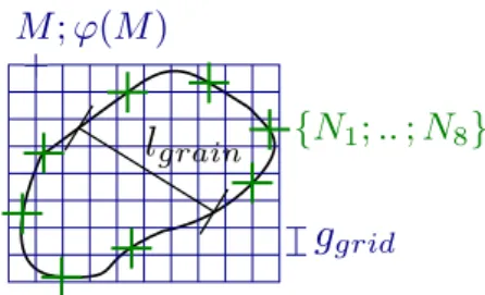
Figure 1: Ingredients of LS-DEM: a cartesian (regular, here) grid with ϕ stored at each grid vertex M , and the boundary nodes Nialong a DE’s surface, satisfying ϕ(~x) = 0. Grid spacing is denoted
ggrid, that is to compare with a characteristic grain size denoted lgrain
being exterior (resp. inner) to the surface. Particle’s surface then corresponds to the zero level set of ϕ. This indirect surface description appears promising in terms of generality. For instance, and contrary to the other DEM extensions based on polyhedra [3], there is no convexity requirement on the grain shape.
No analytical expression for ϕ is even required. Instead, discrete ϕ-values are stored on a DE-centered cartesian grid (Fig. 1), giving ϕ(~x) for all points ~x within the grid using a trilinear interpolation from surrounding grid vertices. From this distance field carried onto the regular grid, a particle’s volume can be obtained in a voxellised fashion, summing grid voxels that are considered inside the particle according to ϕ-values at the eight voxel vertices. Inertial quantities of DE directly come, summing the inertial contributions of these voxels.
Contact detection between such DEs additionally require boundary nodes Ni that are located
along particle’s surface, satisfying ϕ(~x) = 0 (Fig. 1). These are obtained through ray tracing [7]: the intersection of a ray, i.e. a half-line originating from a particle’s center (of mass), with the surface S can be obtained solving for the roots of a cubic polynom corresponding to the distance expression in any grid voxel, after trilinear interpolation. For contact investigation between two DEs labelled 1 and 2, all boundary nodes Niof DE 1 are considered, focusing on the distance value
to DE 2 for each of them.
In more details, a contact between 1 and 2 is detected for a positive node-to-surface distance un:
un= − min(ϕ2(Ni), Ni∈ S1) = −ϕ2(Nc) ≥ 0 (1)
We recall that artificial overlapping regions are permitted in DEM, through a small particle’s interpretation un> 0. In reality, an overlap would correspond to the two particle’s centers getting
closer to each other, while negligible changes in shape would accomodate this normal relative displacement. Once the greatest penetration, at the node Nc, is known, contact laws relate the
normal (resp. tangential) contact force Fn (resp. Ft) to the normal (resp. tangential) relative
displacement un (resp. ut). At this contact scale, LS-DEM considers DEM classical constitutive
relations, being linear elastic in nature with a zero tensile strength threshold along the normal direction, and a additional plastic Coulombian friction threshold along the tangential direction:
Fn = knun; un≥0 (2)
Ft= min(ktut; µ Fn) (3)
with kn (resp. kt) the normal (resp. tangential) stiffness, and µ the friction coefficient. For the
purpose of defining the required normal and tangential directions entering these interaction laws, the contact normal direction is defined as the outwards normal to 1:
~n = ~∇ϕ1(Nc) (4)
To conclude, it is to mention that the regular grid with its distance field, together with the boundary nodes that enter contact treatment, are defined only once at the beginning of a sim-ulation, for reference configurations of the DEs. Those being considered as rigid, the LS-DEM ingredients remain valid for the whole simulation, accounting for rigid bodies transformations.
Figure 2: The spherical packing under triaxial loading, for DEM vs LS-DEM comparison 0 5 10 15 20 0 5 10 15 20 25 30 35 40 45 0 5 10 15 20 0 5 10 15 20 25 30 35 40 45
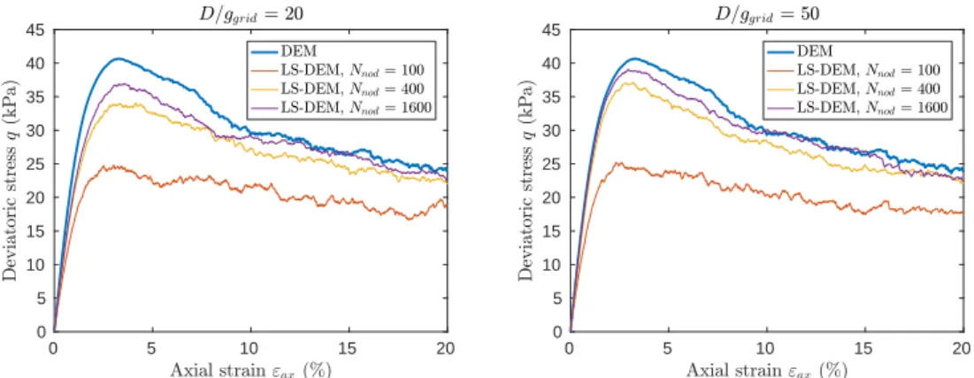
Figure 3: DEM vs LS-DEM comparison in terms of q(εax), for a grid precision equal to 20 (left)
or 50 (right)
3
Computational costs of LS-DEM with regular grids
After being implemented into the YADE code, LS-DEM is herein compared with DEM for a reference case of spherical particles, with the objective of validating the implementation and inves-tigating the associated increase in computational cost. We consider the quasi-static axisymmet-ric compression of a dense packing of 8000 spheres (Fig. 2), under constant lateral confinement: ˙εzz= cst, σxx= σyy= σlat= 20 kPa and starting from an isotropic state σxx= σyy= σzz= σlat.
Boundary conditions are applied through rigid frictionless walls, such that (~x, ~y, ~z) are the principal axes. The mechanical response is described using the axial strain εax= εzz, the volumetric strain
εV = εxx+ εyy+ εzz= εax+ 2 εlatand the deviatoric stress q = σax−σlat. This so-called triaxial
loading is classical in geotechnical engineering, to study the bearing capacity of granular soils. The simulation is carried using both DEM and LS-DEM, with the same contact properties kn, ktand
µ. From the initial isotropic state of the DEM model, positions and radii of the spherical particles are used to define the initial state of an equivalent LS-DEM sample. Distance fields are defined for each spherical particle of diameter D, using a regular grid with a given spacing ggrid i.e. a
given precision lgrain/ggrid= D/ggrid. A given number of boundary nodes, Nnod, is also defined,
using an optimal repartition of those nodes over the spherical surface, following a spiral path as described in [8].
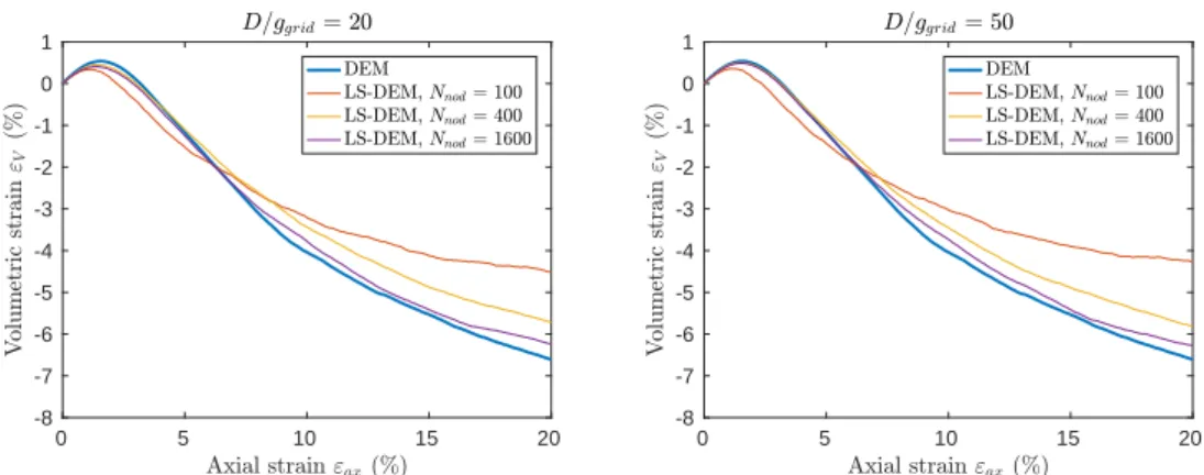
DEM and LS-DEM results are compared in the Figs. 3 and 4. The comparison first vali-dates the approach since LS-DEM results indeed tend to the reference DEM results for sufficient grid fineness and nodes number. As a matter of fact, one can say that obtained precisions for the LS-DEM here vary between 61.0% and 96.1%, quantifying such a LS-DEM precision through max(q)/ max(q)DEM, where max(q)DEM is a reference bearing capacity as obtained in DEM and
where a 100% precision would correspond to an exact match between DEM and LS-DEM. As-sociated computational costs are considerable, be it in terms of time (Fig. 5) or memory (RAM, Fig. 6). Time costs are quantified in wall clock time per numerical timestep. Reference DEM time
0 5 10 15 20 -8 -7 -6 -5 -4 -3 -2 -1 0 1 0 5 10 15 20 -8 -7 -6 -5 -4 -3 -2 -1 0 1
Figure 4: DEM vs LS-DEM comparison in terms of εV(εax), for a grid precision equal to 20 (left)
or 50 (right) 0.6 0.7 0.8 0.9 1 0 20 40 60 80 100 120 140
Figure 5: Increase in time cost for LS-DEM with respect to DEM.
0.6 0.7 0.8 0.9 1 0 200 400 600 800 1000 1200
Figure 6: Increase in RAM cost for packing definition in LS-DEM with respect to DEM.
cost is 22 ms per iteration, for a total time cost of the simulation in the order of 45 min, using one thread on a i7-7700 3.6 GHz processor. Reference DEM RAM cost is 10.7 MB. Both increase by 2 or 3 orders of magnitude for a reasonable precision to be achieved in LS-DEM, turning a simple simulation with evaluation costs in order of hours and megabytes RAM requirements, into a massive one needing several days and gigabytes.
4
Quadtree/Octree data structure
The strong increase in RAM and time computational costs connected to passing from DEM to LS-DEM is arguably related with the uniform Cartesian grid serving as a data structure needed for the φ field definition. Discarding the Cartesian grid is the main point to investigate in order to reduce these costs.
A way to mitigate the need of a Cartesian grid is to use a Quadtree structure for 2D and Octree for 3D representations of DEs. The Quadtree representation for 2D Cartesian object is widely used for images [9] as well as Octree for 3D objects [10]. It allows to define a Cartesian representation for a given level in the tree. At each point of the tree is associated a Cartesian cell and the LS function evaluated in the center of the cell is stored for this point of the tree. The root of the tree represents a cell containing the grain. The size of this cell is stored outside the tree. Each cell is divided in two parts for each space direction leading to 4 children in 2D and 8 children in 3D. Each child has the same tree structure and defines the divided cell. The size of such a cell is known according to the level in the tree (number of parents to attain the root) and the size of the root cell. When a cell does not contain the interface of the grain, no subtree is constructed and this cell is a leave of the tree. Such a cell can have a big size compare to the finest cell. It allows a wide storage reduction compare to the uniform Cartesian grid whose size is the same as the one
Furthermore, Quadtree/Octree data structures allow for efficient leaves searching algorithms. In the following, effects of replacing the Cartesian grid by Quadtree/Octree data structures on the memory and walltime requirements of LS-DEM simulations will be evaluated.
4.1
Memory cost reduction with Quadtree/Octree
The Level Set information defined on the uniform grid is a rich information which can be conserved on a reduced tree structure. Each cell which does not contain the grain interface has no reason to contain subcell (child) and the information of the signed distance function ϕ at the center of the cell is sufficient. This value is even sufficient to determine if this cell can or can not contain the interface. Without loss of information for the LS-DEM, the Quadtree/Octree of the Level Set function can replace the tabular of the Level Set function on the uniform grid. Note that the Quadtree/Octree structure allows to know the coordinates of a point of the tree according to the position in the tree, the root position and the root cell size. Then, only the Level Set function ϕ is stored and the storage of the Level Set function looks like the following tree:
ϕ b ϕ b ϕ b ϕ b ϕ b ϕ b ϕ b ϕ∗ b ϕ b ϕ b ϕ b ϕ b ϕ b ϕ b ϕ b ϕ b ϕ∗∗ b ϕ b ϕ b ϕ b ϕ b
At the finest level of grid, at least one of the leaves of a same father contains the interface and can be considered as a point of the interface up to the projection along ∇ϕ. This consideration can replace the ray tracing method to define the Ninodes
of the interface (Fig. 1).
Imagine that ϕ∗, ϕ∗∗ are the only leaves
to satisfy −d < ϕ∗, ϕ∗∗ < 0 where d
is the finest grid size (or half finest grid size). Then, these leaves can be consid-ered as the leaves of interest (LI) defining the nodes of the interface.
On the left side of Figure 7, the centers of all the cells of a Quadtree (depth 9) are plotted. On the right side, we show only the leaves of interest corresponding to the interface nodes.
−1.00 −0.75 −0.50 −0.25 0.00 0.25 0.50 0.75 1.00 −1.00 −0.75 −0.50 −0.25 0.00 0.25 0.50 0.75 1.00 −1.00 −0.75 −0.50 −0.25 0.00 0.25 0.50 0.75 1.00 −1.00 −0.75 −0.50 −0.25 0.00 0.25 0.50 0.75 1.00
Figure 7: Cell centers of the Quadtree of the Level Set for a 2D particule on the left. Nodes of the interface as LI of the Quadtree on the right
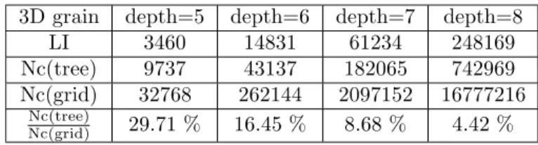
The reduction in simulation storage requirements can be qualitatively evaluated by comparing the data shown in Figure 7 to the corresponding uniform Cartesian grid. A quantitative evaluation of memory cost reduction for the particle shown in Figure 7 is given in Table 1. The notation Nc(tree) means the number of cells in the Quadtree/Octree and Nc(grid) is the number of cells on the associated uniform grid.
2D grain depth=5 depth=6 depth=7 depth=8 depth=9 depth=10 LI 112 249 515 1051 2031 4143 Nc(tree) 413 1041 2265 4857 9953 20265 Nc(grid) 1024 4096 16384 65536 262144 1048576 Nc(tree) Nc(grid) 40.33 % 25.42 % 13.82 % 7.41 % 3.8% 1.93 %
Table 1: Comparison of data storage for a 2D grain.
The tree depth 7 is sufficient according to section 3 and leads to important RAM cost reduction. With a 3D grain, the gains are even more important and crucial for the problem as shown in Table 2.
3D grain depth=5 depth=6 depth=7 depth=8
LI 3460 14831 61234 248169
Nc(tree) 9737 43137 182065 742969
Nc(grid) 32768 262144 2097152 16777216
Nc(tree)
Nc(grid) 29.71 % 16.45 % 8.68 % 4.42 %
Table 2: Comparison of data storage for a 3D grain.
4.2
Level Set intersection
The data of the Level Set function stored in the Quadtree/Octree suffice to evaluate the distance to the boundary for a given point. This result is precise close to the interface and sufficiently accurate far from the interface. This tree structure is then used instead of a regular grid. The decrease in RAM consumption achieved by replacing the uniform grid by Quadtree/Octree was shown in the previous section. The simulation time may be reduced leveraging the same principles of tree structures. We are interested in computing the overlaps of two Quadtrees/Octrees to identify which leaves of interest meet a cell of the other tree with negative ϕ. The recursive algorithm works first on coarse cells and then on finer cells only if an intersection is possible. We construct such an algorithm with the proposed Quadtree/Octree including LI. We also optimize this algorithm to extract a tree structure to attain only LI. Such a tree is detailed below.
Quadtree structure b b b b b b b b b LI b b b b b b b LI b LI b b b b b b LI b LI b
Reduced unstructured tree (RUT) This tree allows to focus on leaves of interest (LI). The position of each child has to be stored as well as the child number of the Quadtree. The coordinate of LI can then be
recon-structed. b 1 b 3 b b 1 3 b 1 b b 0 b 1 3 b b 1 b 2
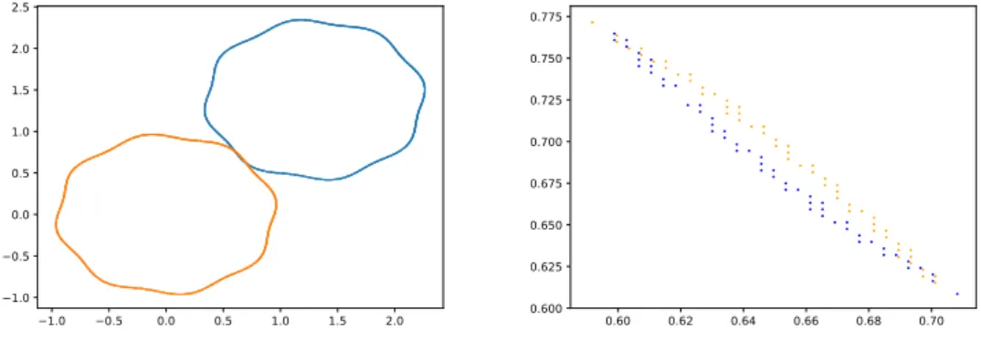
The nodes of the interface LI of a grain A which penetrates a grain B can then be computed with Quadtree/Octree A and Quadtree/Octree B or with RUT A and Quadtree/Octree B. The computational cost to identify overlapping nodes with these two structures are then compared with the direct approach consisting of testing each interface node. The graphical result of the overlapping algorithm is presented in Figure 8 for the tree depth of 9. On the right, the LI are the
−1.0 −0.5 0.0 0.5 1.0 1.5 2.0 −1.0 −0.5 0.0 0.5 1.0 1.5 2.0 2.5 0.60 0.62 0.64 0.66 0.68 0.70 0.600 0.625 0.650 0.675 0.700 0.725 0.750 0.775
Figure 8: All LI for two particules are plotted on the left. Only overlapping LI, resulting from the overlap algorithms, are plotted on the right
The computational cost is introduced as a percentage of the computational cost of the direct method. The direct method used in LS-DEM tests all the interface nodes of A, which are not too far apart, to evaluate the Level Set function of the grain B.
Tests were done for 2D and 3D non-spherical grains with slight overlaps similar to the ones occurring in LS-DEM. The number of LI overlapping the other grain is denoted ”LI overlapping” in Table 3. The ”relative time 1” means the relative time with Quadtree/Octree structure to represent LI, The ”relative time 2” means the relative time with the algorithm based on RUT structureLI.
The tests are done with Python3 and show some variations with respect to time computation. These results are reproductible with relative variations of order of 10%. Nevertheless, it clearly shows that with 2D grains, the Quadtree approach is not sufficient to represent LI to achieve a speed-up of the computation. Benefits of the algorithm would be obtained for too fine grids. But the improved algorithm, where the data structure to store LI is an unstructured tree, shows an interesting time cost reduction. A much more important gain is obtained with 3D grains even for coarse grids. Benefits are obtained with the two data structures and unstructured trees also have to be preferred.
2D grain depth=5 depth=6 depth=7 depth=8 depth=9 depth=10
LI overlapping 0 0 6 21 55 128
Relative time 1 260 % 276 % 165 % 177% 130 % 106%
Relative time 2 104 % 65% 44 % 39 % 30 % 22%
3D grain depth=5 depth=6 depth=7 depth=8
LI overlapping 0 8 38 670
Relative time 1 66 % 38 % 22 % 13%
Relative time 2 18 % 8 % 5.8 % 3.8%
Table 3: Relative times of he overlap algorithms with Quadtree/Octree structure and RUT struc-ture compared to the direct method.
5
Conclusion
Leveraging the Level Set representation of a grain surface, the Level Set-Discrete Element Method (LS-DEM) is an already proven technique for simulations of granular media without limitations on the grain shape [4, 5]. However, LS-DEM is computationally significantly more expensive than standard DEM codes. In the present paper, we first validated our implementation of LS-DEM in the YADE code and confirmed the steep increase of simulation costs connected to replacing DEM by LS-DEM. Next, an attempt was made to reduce the computational costs of LS-DEM by
replacing the uniform Cartesian grid needed for the LS grain representation by Quadtree/Octree data structures. The results suggest up to 91% of RAM and 94% of simulation time could be saved in 3D using tree-like data structures, for a Cartesian grid of 1283points. In the following work, the
new algorithms will be implemented into the YADE code, enabling lighter LS-DEM simulations. Acknowledgment
Financial support from French Sud Region to the LS-ENROC project is gratefully acknowledged, together with fruitful discussions with S. Bonelli (INRAE) and F. Golay (Univ. Toulon).
References
[1] Cundall, P. & Strack, O.: A discrete numerical model for granular assemblies. G´eotechnique, vol. 29: (1979) pp. 47–65. doi:10.1680/geot.1979.29.1.47.
[2] Duriez, J. & Wan, R.: Stress in wet granular media with interfaces via homogenization and discrete element approaches. Journal of Engineering Mechanics, vol. 142, no. 12: (2016) doi:10.1061/(ASCE)EM.1943-7889.0001163.
[3] Cundall, P.: Formulation of a three-dimensional distinct element model–Part I. A scheme to detect and represent contacts in a system composed of many polyhedral blocks. International Journal of Rock Mechanics and Mining Sciences & Geomechanics Abstracts, vol. 25, no. 3: (1988) pp. 107 – 116. doi:10.1016/0148-9062(88)92293-0.
[4] Jerves, A. X., Kawamoto, R. Y. & Andrade, J. E.: Effects of grain morphology on criti-cal state: a computational analysis. Acta Geotechnica, vol. 11, no. 3: (2016) pp. 493–503. doi:10.1007/s11440-015-0422-8.
[5] Kawamoto, R. Y., And`o, E., Viggiani, G. & Andrade, J. E.: Level set discrete element method for three-dimensional computations with triaxial case study. Journal of the Mechanics and Physics of Solids, vol. 91: (2016) pp. 1–13. doi:10.1016/j.jmps.2016.02.021.
[6] ˇSmilauer, V. et al.: Yade Documentation 2nd ed. The Yade Project: (2015). http://yade-dem.org/doc/ doi:10.5281/zenodo.34073.
[7] Lin, C.-C. & Ching, Y.-T.: An efficient volume-rendering algorithm with an analytic approach. The Visual Computer, vol. 12, no. 10: (1996) pp. 515–526. doi:10.1007/s003710050083. [8] Rakhmanov, E. A., Saff, E. B. & Zhou, Y. M.: Minimal discrete energy on the sphere,
Mathe-matical Research Letters, vol. 1: (1994) pp. 647–662. doi:10.4310/MRL.1994.v1.n6.a3.
[9] Sullivan, G. J. & Baker, R. L.: Efficient quadtree coding of images and video. IEEE Transac-tions on Image Processing, vol. 3, no. 3: (1994) pp. 327–331. doi:10.1109/83.287030
[10] Potmesil, M.: Generating octree models of 3D objects from their silhouettes in a sequence of images. Computer Vision, Graphics, and Image Processing, vol. 40, no. 1: (1987) pp. 1–29. doi:10.1016/0734-189X(87)90053-3
[11] Jung, D. & Gupta, K. K.: Octree-based hierarchical distance maps for collision detection. Proceedings of IEEE International Conference on Robotics and Automation, Minneapolis, MN, USA, vol. 1: (1996) pp. 454–459. doi: 10.1109/ROBOT.1996.503818
[12] Losasso, F., Gibou, F. & Fedkiw, R.: Simulating Water and Smoke with an Octree Data Structure. ACM Trans. Graph., vol. 23: (2004) pp. 457–462. doi:10.1145/1015706.1015745 [13] Guittet, A., Theillard, M. & Gibou, F.: A stable projection method for the incompressible
NavierStokes equations on arbitrary geometries and adaptive Quad/Octrees. Journal of Com-putational Physics, vol. 292: (2015) pp. 215–238. doi:10.1016/j.jcp.2015.03.024