Discrete Generalized Multigroup Theory and Applications
By Lei Zhu
B5.Eng. Engineering Pnysics, I singnua university, 2005 M.S. Nuclear Engineering, Texas A&M University, 2008 Submitted to the Department of Nuclear Science and Engineering in-
Partial Fulfillment of the Requirement for the Degree of Doctor of Philosophy in Nuclear Science and Engineering
at the
MASSACHUSETTS INSTITUTE OF TECHNOLOGY
February 2012
@ Massachusetts Institute of Technology. All rights reserved
I .
Signature of Author:
Certified by:
Certified by:
Accepted by:.
Department of Nuclear Science and Engineering
November 8, 2011
/7
__
enoit Forget
-
Thesis Supervisor
Assint Professor of Nuclear Science and Engineering
Kord S. Smith - Thesis Reader
KEPCO Professor of the Practice of Nuclear Science and Engineering
Mujid S. Kazimi
TEPCO Prof, oe Nuclear Engineering Chair, Department Committee on Graduate StudentsDiscrete Generalized Multigroup Theory and Applications
By
Lei Zhu
Submitted to the Department of Nuclear Science and Engineering on November 8, 2011, in Partial Fulfillment of the
Requirements for the degree of Doctor of Philosophy in Nuclear Science and Engineering
ABSTRACT
This study develops a fundamentally new discrete generalized multigroup energy expansion theory for the linear Boltzmann transport equation. Discrete orthogonal polynomials are used, in conjunction with the traditional multigroup representation, to expand the energy dependence of the angular flux into a set of flux moments. The leading (zeroth) order equation is identical to a standard coarse group solution, while the higher order equations are decoupled from each other and only depend on the leading order
solution due to the orthogonality property of the discrete Legendre polynomials selected. This decoupling leads to computational times comparable to the coarse group calculation but provides an accurate fine group energy spectrum. A source update process is also
introduced which provides improvement of integral quantities such as eigenvalue and reaction rates over the coarse group solution.
An online energy recondensation methodology is proposed to improve traditional
multilevel approach in reactor core simulations. Since the discrete generalized multigroup (DGM) method produces an unfolded flux with a fine group structure, this flux can then be used to recondense the coarse group cross-sections using the obtained core level fine group DGM solution, which can be done iteratively. Computational tests on light water reactors and high temperature reactors are performed. Results indicate that flux can fully converge to the fine group solution with a computational time less than that of standard fine group calculation as long as a flat angular flux approximation is used spatially. The recondensation concept is extended to a nonlinear energy acceleration form. The method can effectively accelerate the fine group calculation by providing a more accurate initial guess provided from a few iterations of DGM recondensation calculation.
Computational results show that the computational time and number of transport sweeps of the accelerated algorithm are much less than those of corresponding standard fine group calculations.
Thesis Supervisor: Benoit Forget
Title: Assistant Professor of Nuclear Science and Engineering Thesis Reader: Kord S. Smith
Acknowledgements
I would like to express my deepest gratitude to my advisor, Prof. Benoit Forget for his continuous support and constructive advices throughout my PhD study at MIT. His encouragements and help have made me really enjoy this research project over the past a few years.
I am deeply grateful to my thesis reader, Prof. Kord Smith for his incredibly helpful discussions and advices. His wide knowledge in computational reactor physics has been of great value to me.
Many thanks to Dr. Thomas Newton for his advice and funding support during my first year of study on the MIT Reactor fuel conversion project. Many thanks to the funding support from the Consortium for Advanced Simulation of Light Water Reactors (CASL) project.
I would like to thank all the professors, staffs, colleagues and friends in the Department of Nuclear Science and Engineering. Additionally, I would like to thank the department for giving me the opportunity to study here.
I would like to thank my parents for their continuous support and love throughout my life. Thanks for their encouragement for my graduate study in the US.
Lastly, I would like to give a special thank to my wife, Shanshan, for her support and love.
Table of Contents
Abstract... ... . 3 Acknowledgements... 4 Table of Contents... 5 List of Figures... 7 List of Tables ... 10 Acronyms... 12 Chapter 1. Introduction... 14 1.1 M otivation... 14 1.2 Objectives ... 15 1.3 Thesis organization... 16Chapter 2. Background and Review ... 18
2.1 Energy related discretization methods in deterministic transport... 18
2.1.1 M ultigroup methodology ... 18
2.1.2 CENTRM and submoment expansion ... 19
2.1.3 RAZOR continuous energy lattice code ... 22
2.1.4 Linear multigroup method ... 22
2.1.5 W avelet energy expansion... 23
2.1.6 Opacity distribution function concept... 25
2.1.7 Energy expansion using continuous orthogonal polynomials ... 26
2.2 Current multilevel approaches in reactor simulations ... 28
2.2.1 General multilevel approaches... 28
2.2.2 Lattice-core online iteration methods ... 30
Chapter 3. Discrete Generalized Multigroup Energy Expansion Theory... 33
3.1 DGM method derivation... 33
3.2 Comparison of discrete and continuous energy expansions ... 41
3.3 Computational results ... 45
3.3.1 One dimensional BWR assembly tests ... 47
3.3.2 One dimensional BW R core tests ... 49
3.3.3 Eigenvalue and fluxes updates... 52
3.4 Summary... 61
4.1 M ethod description ... 64
4.2 Com putational results ... 70
4.2.1 One dim ensional BW R core tests ... 70
4.2.2 One dim ensional HTR core tests ... 81
4.2.3 Two dim ensional PW R core tests... 96
4.2.4 Two dim ensional HTR core tests... 106
4.3 M ore discussions on recondensation ... 115
4.3.1 Spatial dependence of the DGM method... 115
4.3.2 Perturbation technique in collision term ... 123
4.3.3 M em ory requirem ent of recondensation... 127
4.4 Summ ary... 128
Chapter 5. Nonlinear Energy Acceleration using DGM method... 130
5.1 M ethod description ... 130
5.2 Com putational results ... 130
5.3 Summ ary... 134
Chapter 6. Summ ary and Future W ork ... 135
6.1 Summ ary... 135
6.2 Future work... 139
Appendix A. Derivation of Standard Multigroup Method... 140
Appendix B. Orthogonal Polynomials... 148
B.1 Continuous orthogonal polynomials... 148
B.2 Discrete orthogonal polynomials ... 150
B.3 Discussion on discrete expansions... 154
Appendix C. Derivation of DGM Method on Diffusion Equation ... 164
Appendix D . Definition of Errors ... 171
Appendix E. Algorithm s of Fixed Point Iterations ... 173
E.1 Algorithm s of power iteration... 173
E.2 Algorithm s of external source problem s... 178
List of Figures
FIGURE Page
2.1 Typical multilevel approach in Light Water Reactor calculations ... 29
2.2 Lattice-core online iteration... 31
3.1 Expansion of a step function using continuous Legendre polynomials... 43
3.2 Expansion of a step function using discrete Legendre polynomials... 44
3.3 47 group cross section condensation... 45
3.4 1-D BWR core and assembly configurations... 46
3.5 Core 1 scalar flux comparison (fast groups)... 57
3.6 Core 1 scalar flux relative error (fast groups)... 57
3.7 Core 1 scalar flux comparison (thermal groups)... 58
3.8 Core 1 scalar flux relative error (thermal groups) ... 58
3.9 Core 3 scalar flux comparison (fast groups)... 59
3.10 Core 3 scalar flux relative error (fast groups)... 59
3.11 Core 3 scalar flux comparison (thermal groups)... 60
3.12 Core 3 scalar flux relative error (thermal groups) ... 60
4.1 Flow chart of the traditional multilevel procedure ... 66
4.2 Flow chart of the recondensation procedure... 67
4.3 Scalar flux rms relative errors of 1-D BWR core 1 ... 76
4.4 Eigenvalue relative errors of 1-D BWR core 1... 76
4.5 Scalar flux nns relative errors of 1-D BWR core 3 ... 77
4.7 Scalar flux comparison for core 3 water region... 78
4.8 Scalar flux relative error for core 3 water region... 79
4.9 Scalar flux comparison for core 3 Fuel (high enrichment) region... 79
4.10 Scalar flux relative error for core 3 Fuel (high enrichment) region... 80
4.11 Scalar flux comparison for core 3 Fuel+Gd region ... 80
4.12 Scalar flux relative error for core 3 Fuel+Gd region ... 81
4.13 1-D HTR core configuration... 82
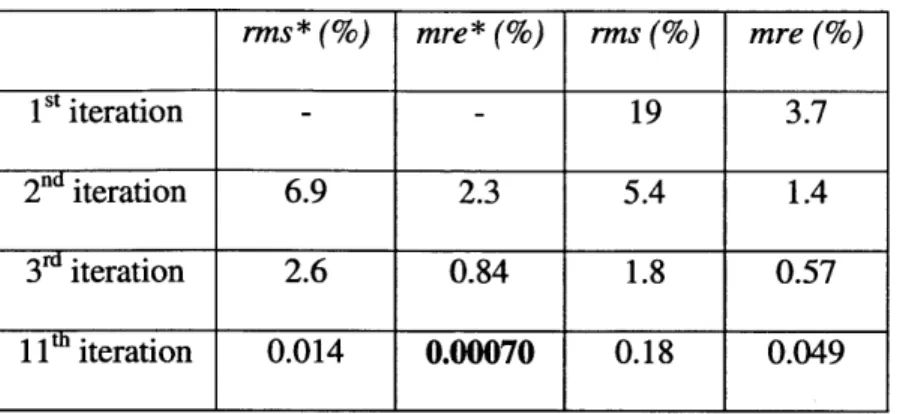
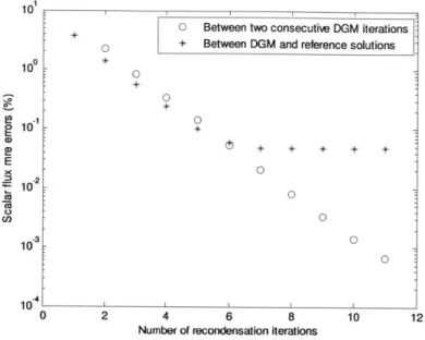
4.14 Scalar flux mre errors... 85
4.15 Eigenvalue relative errors ... 85
4.16 Average flux on the Graphite/Fuel 1 interface ... 86
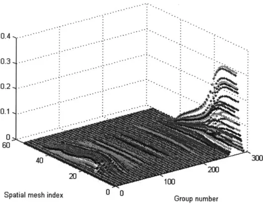
4.17 Scalar flux 295 group solution on full space and energy mesh ... 87
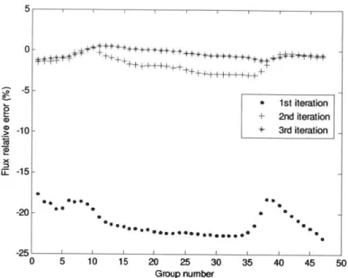
4.18 Fission rate relative error in the first 3 DGM iterations ... 88
4.19 Absorption rate relative error in the first 3 DGM iterations ... 89
4.20 Group 1 flux spatial distribution... 90
4.21 Group 2 flux spatial distribution... 90
4.22 Group 50 flux spatial distribution... 91
4.23 Group 150 flux spatial distribution... 91
4.24 Group 275 flux spatial distribution... 92
4.25 Group 295 flux spatial distribution... 92
4.26 Scalar flux mre errors... 95
4.27 Eigenvalue relative errors ... 95
4.28 Overview of 2-D PWR core configuration... 96
4.30 Fuel pin approximation in Cartesian geometry... 97
4.31 Scalar flux nns relative errors of 70 group 2-D PWR core ... 102
4.32 Eigenvalue relative errors of 70 group 2-D PWR core... 102
4.33 Fission density relative error (%) for 1t DGM iteration... 103
4.34 Fission density relative error (%) for 2nd DGM iteration... 104
4.35 Fission density relative error (%) for 3rd DGM iteration ... 105
4.36 Fission density relative error (%) for 4th DGM iteration ... 105
4.37 Fission density relative error (%) for 13'h DGM iteration ... 105
4.38 2-D HTR core configuration... 106
4.39 Scalar flux mre relative errors of 26 group 2-D HTR core... 109
4.40 Eigenvalue relative errors of 26 group 2-D HTR core ... 110
4.41 Fission density distribution of 26 group 2-D HTR core ... 111
4.42 Fission density relative error (%) for 1" DGM iteration... 112
4.43 Fission density relative error (%) for 2nd DGM iteration... 112
4.44 Fission density relative error (%) for 3rd DGM iteration... 113
4.45 Fission density relative error (%) for 4t DGM iteration ... 113
4.46 Fission density relative error (%) for 5b DGM iteration ... 114
4.47 Fission density relative error (%) for 38t DGM iteration ... 114
4.48 Scalar flux nns relative error of 1-D BWR core l (SC vs. SD)... 122
4.49 Eigenvalue relative error of 1-D BWR core 1 (SC vs. SD)... 123
List of Tables
TABLE Page
3.1 Assemblies 1 and 4 eigenvalue and computational time ... 48
3.2 Assembly 1 DGM result errors ... 48
3.3 Assembly 4 DGM result errors... 48
3.4 Cores 1 and 3 eigenvalue and computational time ... 50
3.5 Core 1 DGM result... 50
3.6 Core 3 DGM result... 51
3.7 Cores 1 and 3 eigenvalue and time after the updates... 54
3.8 Core 1 DGM result after the updates ... 54
3.9 Core 3 DGM result after the updates... 55
4.1 l-D BWR Core 1 errors in fluxes ... 72
4.2 1-D BWR Core 1 computational results ... 73
4.3 1-D BWR Core 3 errors in fluxes... 73
4.4 1-D BWR Core 3 computational results ... 74
4.5 1-D HTR core configuration... 82
4.6 1D HTR errors in fluxes ... 84
4.7 ID HTR eigenvalue and computational time... 84
4.8 ID HTR (anisotropic) errors in fluxes... 94
4.9 ID HTR (anisotropic) eigenvalue and computational time ... 94
4.10 70 group 2-D PWR core errors in fluxes ... 98
4.12 70 group 2-D PWR core computational results ... 101
4.13 26 group 2-D HTR core errors in fluxes... 108
4.14 26 group 2-D HTR core computational results... 109
4.15 1-D BWR Core 1 errors in fluxes (step characteristics)... 120
4.16 1-D BWR Core 1 computational results (step characteristics)... 121
5.1 3 coarse group with expansions acceleration results ... 132
5.2 2 coarse group with expansions acceleration results ... 133
6.1 Recondensation result summary ... 137
B.1 Double precision DLOP values of N=4 ... 156
B.2 Exact and reconstructed step functions (1)... 157
B.3 Exact and reconstructed step functions (2)... 158
B.4 Discrete polynomial expansion of step function (N=50)... 160
Acronyms
BWR Boiling Water Reactor
CENTRM Continuous ENergy TRansport Module CMFD Coarse Mesh Finite Difference
DGM Discrete Generalized Multigroup Method DLOP Discrete Legendre Orthogonal Polynomials
DRAGON A collision probability transport code for cell and supercell calculations DSA Diffusion Synthetic Acceleration
DT Discrete Tchebichef Polynomials ENDF Evaluated Nuclear Data File
Gd Gadolinium
GS Gauss-Seidel
HELIOS A lattice physics code HTR High Temperature Reactors
IEEE Institute of Electrical and Electronics Engineers IGDM Iterative Transport-Diffusion Methodology
LWR Light Water Reactors
MCNP Monte Carlo N-Particle MOC Method of Characteristics
MOX Mixed Oxide Fuel
MRE Mean Relative Error
ODF Opacity Distribution Function
PI Power Iteration
PWR Pressurized Water Reactor RMS Root Mean Square Relative Error
SCALE Standardized Computer Analyses for Licensing Evaluation
SC Step Characteristics
SD Step Difference
Sn Discrete Ordinates
Chapter 1. Introduction
1.1 Motivation
Current core-level deterministic methods rely entirely on the multigroup energy treatment of the nuclear cross-sections [Bell 1970] [Henry 1975] [Duderstadt 1976] [Lamarsh 1983] [Hebert 2009]. In the energy condensation process, continuous energy data is condensed in a more manageable multigroup format through multiple levels of approximation to eventually produce a reduced-complexity dataset with which the core calculation can be performed efficiently. Reaction rates are conserved based on the knowledge of the exact energy spectrum. Since this quantity is unknown a priori, a multilevel approach is used to refine the flux spectrum approximation which is then used to condense the cross-sections into a smaller number of groups.
As the number of energy groups is reduced, spatial detail is added often going from a 1-D pin cell to a 2-D fuel assembly to an eventual full 3-D core. This multilevel approach generally assumes that strong spectral effects are local and can be approximated coarsely as the spatial size increases to reduce computational costs. As the level of heterogeneity increases in nuclear reactor core designs, this assumption breaks down and requires
adjustments.
used in Fast Reactors. While such an approach has proven sufficient for current reactors for which many experiments were performed, it is envisioned that high-fidelity core modeling will require thousands of energy groups if one desires to improve the predictive capability of the simulation. Increasing the number of energy groups allows for a better representation of the resonance region and a more accurate spectral description but comes with a substantial computational cost which is proportional to the number of energy
groups.
In particle transport problems, the neutron flux is a function of space, angle, energy and time. The nuclear community has put much effort on development of different spatial and angular discretization methods and associated acceleration algorithms, while less effort has been put on the energy discretization methods. The dominant treatment of the energy dependence is the multigroup method, especially at the core level.
The goal of this dissertation is to develop an energy treatment for the neutron transport equation that reduces the computational cost needed for high-fidelity modeling of nuclear reactors.
1.2 Objectives
The main objective of this work is to develop a new energy discretization approach that reduces reliance on the multilevel approach (i.e. ID pin cell, 2D lattice, 3D core). The
and eliminate the need for pin cell or lattice level calculations. Additionally this new approach must remain computationally competitive with current few group strategy and fit in the framework of common deterministic transport methods.
1.3 Thesis organization
This thesis is organized as follows. Chapter 2 reviews existing methods and includes four subsections. Section 2.1 briefly reviews the existing energy variable discretization methodologies in deterministic transport theory. Section 2.2 reviews existing lattice-core level iterations methods.
Chapter 3 is dedicated to the Discrete Generalized Multigroup (DGM) method. Section 3.1 derives the DGM form of the transport equation. Section 3.2 compares discrete and continuous energy expansions and illustrates the advantages of discrete expansions. Section 3.3 shows computational results for 1-D BWR assemblies and cores tests. Section 3.4 summarizes important findings.
Chapter 4 develops the online recondensation methodology with computational results. Section 4.1 describes the method while Section 4.2 presents the computational results of this extension. Section 4.3 discusses limitations of DGM recondensation from the perspective of spatial discretization and accuracy of the perturbation technique used in the collision term, and briefly analyzes memory requirement of recondensation. Section 4.4 provides a brief summary of the chapter.
Chapter 5 develops an energy acceleration method based on the recondensation result as an initial guess for fine group calculation.
Chapter 6 summarizes the theories and methodologies developed in this work, followed by a discussion of possible future work and directions.
Chapter 2. Background and Review
This chapter first reviews existing energy discretization methods in deterministic radiation transport theory, followed by the multilevel approach using the multigroup energy discretization simulations and lattice-core level iteration methods. The third section reviews energy related acceleration methods, followed by a review of orthogonal polynomials.
2.1 Energy related discretization methods in deterministic transport
2.1.1 Multigroup methodology
Current core-level deterministic methods rely exclusively on the multigroup energy treatment of the nuclear cross-sections [Bell 1970] [Henry 1975] [Duderstadt 1976] [Lamarsh 1983] [Hebert 2009]. The multigroup discretization divides the energy domain into G energy intervals. Group flux is defined as an integral quantity within each group, and group cross sections are defined as an average value over each group using an approximate flux spectrum as the weighting function.
Since the discrete generalized multigroup method is closely related to the standard multigroup method, a brief derivation from continuous energy to the standard multigroup form of the transport equation is given in Appendix A. The key aspect is the definition of
the group cross sections which are averaged cross sections within a group weighted by the exact flux spectrum:
Eg-_
f a(E)f(E)dE
a
E (2.1)ff (E)dE
E,
For a problem with defined geometry and composition, the only way to obtain accurate multigroup cross sections is to know the exact flux spectrum f(E) within each group which should also depend on space and angle in heterogeneous problems. Unfortunately this spectrum is not known and approximation is needed. Errors in this approximation are the major cause of uncertainty associated with the multigroup method. The flux spectrum is very sensitive to the isotope concentration and spatial dependence, especially when resonances are present. A phenomenon known as self-shielding occurs, which refers to a change in resonance absorption due to spatial and spectral variations of the neutron flux. Self-shielding effects should be considered in the processing of nuclear cross section data. The following sub-sections briefly review alternative energy discretization methods in the literature.
2.1.2 CENTRM and submoment expansion
An alternate approach to the multigroup method is the use of pointwise cross section data [Ching 1976] [Liu 1981]. Williams et al developed the 1 -D discrete ordinates code
CENTRM for nuclear data processing that treats part of the nuclear data as pointwise cross-sections [Williams 1995] [Williams 2009]. The method uses a combination of multigroup and pointwise treatments to obtain a very accurate pointwise neutron
spectrum. The "submoment" expansion technique is used to accurately evaluate the scattering transfer function. CENTRM is currently used in the SCALE [Bowman 2007] package to generate resonance shielded multigroup data. The code solves a fixed source transport equation in infinite media or 1-D pin-type geometries.
The full energy range (0-20MeV) is divided into 3 intervals, i.e., Upper Multigroup Range (UMR), Pointwise Range (PW) and Lower Multigroup Range (LMR). Flux calculations in the 3 intervals are coupled through the scattering sources. The PW region is chosen to be above the thermal energy range and to include all the resolved resonances of important isotopes, i.e., 4eV-10keV. In particular, the PW region should be below the inelastic scatter threshold of all significant materials. UMR and LMR are regions where cross sections have much smoother variation where multigroup calculations are
performed.
Results from CENTRM provide a pointwise energy flux spectrum on a fine energy structure (-30,000-70,000 discrete points) and thus greatly improves the energy resolution. The discrete pointwise flux is then used as weighting function for PMC
[Williams 2009, 2], a module in Scale to process results from CENTRM, to generate self-shielded group cross sections used for higher spatial dimensional calculations.
spectrum for the treatment of resolved resonances than NITAWL [Greene 2009], the prior module used for self-shielding in SCALE which uses the Nordheim Integral method [Hollenback 1998].
A special consideration in CENTRM is that in the expression of spherical harmonic moments of elastic and inelastic (if included) scattering sources, the integrand contains coupling of the initial and final energy of the scattered neutrons which make the overall algorithm very inefficient. Thus a submoment expansion method was proposed to evaluate the anisotropic scattering source efficiently under this pointwise transport framework [Williams 2000].
In order to decouple the initial and final energy dependence in the integrand of scattering source moments, this spherical harmonic scattering source moment is further expanded in a series of factored submoments. This double expansion facilitates the treatment of the scattering sources but introduces numerical instability for heavy nuclides that require high angular expansion. The total number of submoments increases rapidly with increasing order of scatter, which limits the order of anisotropic scattering.
CENTRM solves one dimensional simple geometry problems, e.g., ID pin cell geometry with a white boundary condition. This representation is an important limitation of this approach. Moreover, due to the fine energy nature of CENTRM, it is difficult to extend to core level calculations where much more spatial details are needed. An extension was proposed for 2D pin cell geometries which showed promise [Zhong 2005] [Zhong 2006].
2.1.3 RAZOR continuous energy lattice code
The RAZOR lattice code proposes a "near-continuous" energy pointwise solution method on the lattice level calculation to generate few-group diffusion constants that account for self-shielding effect [Zerkle 1997]. This method was developed to improve the resonance energy treatment within the multigroup methodology and uses pointwise data to generate the multigroup data. RAZOR solves one and two dimensional fixed source neutron transport problems.
Continuous energy transport is used in both fast and thermal energy ranges. In the slowing down algorithm a "dual energy resolution" was developed to obtain detailed energy resolution while at the same time reducing memory requirements by a combination of fine and coarse group slowing down buffers.
Similar to CENTRM, RAZOR and these lattice level codes with detailed energy
treatments are difficult to extend to core level calculations due to the high computational resource requirements.
2.1.4 Wavelet energy expansion
A wavelet function expansion method was developed for the treatment of self-shielding effect [Wu 2010]. Similar to CENTRM, the non-resonance energy ranges use standard multigroup method. In the resonance range, the energy is divided into many group
intervals. The energy dependence of angular flux is then expanded using Daubechies' wavelet scaling function [Daubechies 1992] to separate energy dependence spectrum with spatial and angular dependence coefficients of the angular flux. A set of equations can be solved for the spatial and angular dependent coefficients using the orthogonality properties of Daubechies' wavelets scaling function. Finally the flux spectrum can be unfolded after obtaining these coefficients.
A program WAVRESON was developed using this methodology with the method of characteristics (MOC). Benchmark problems with infinite homogeneous medium, single pin and cylindrical cluster geometries were tested and results showed that this method can give errors on the order of less than one percent on k-infinity by comparing with MCNP reference solutions.
A disadvantage of the method is the computational burden because the angular flux needs to be expanded to high orders. Within each of the resonance energy intervals, many coefficient equations need be solved. The detailed energy treatment makes it difficult to be applied to complex geometry problems.
2.1.5 Linear multigroup method
A linear multigroup method was developed [Attieh 2002] [Attieh 2004]. The standard multigroup method is assumed to have a piecewise constant spectrum within each group, i.e.,
fg(E)=1, EE[E,E_] (2.2)
=0, else.
Under this assumption, the authors proposed a generalized member function; in particular,
the linear multigroup method assumes a hat basis function to give the spectrum a linear
dependence within each group:
fg(E)=
E- Eg**
EE [Eg+,,,Eg]g g+(3
, E e[Eg,Eg,]. E,_, - E,
This shape function is similar to the linear basis function used in continuous finite
element method, thus the name Linear Multigroup (LMG) method. With this linear shape
function, the LMG cross sections were generated by modifying NJOY modules and the
resulting cross sections were used to solve for gamma ray fluxes and absorption rates in
different energy groups.
The proposed LMG method was tested on two gamma ray spectrum calculations in
infinite homogeneous oxygen medium, with continuous spectrum and monoenergetic
sources, respectively. The results from multigroup and LMG with the same number of
energy groups were compared. Results showed that errors with the LMG or a
method, given the same multigroup energy structure. With the increase of number of energy groups, the new approaches converge faster than the multigroup method.
There are a few issues with this method. Firstly, due to the overlapping of basis functions in a particular group, the total cross section has "group-to-group" dependence which is non-physical, i.e., instead of a, in a group, .,g_, qg and ,) exist in a group. The generation of these pseudo cross sections requires extra computational effort. Moreover,
solving the linear system with these extra pseudo entries also require more computational effort. The scattering matrix similarly has non-physical entries for scattering from each
group to the next higher group (named "fictitious upscattering") for each group, which makes the scattering matrix denser than the standard multigroup method and thus requires more computational effort to solve.
Secondly, this method is tested in the infinite homogeneous medium, and it can be applied in shielding problems, as well as the early stage of cross section processing with ultra-fine energy groups when the standard multigroup method is assumed to have a constant shape function within each energy group. The extension of the method to core level simulation would be difficult.
2.1.6 Opacity distribution function concept
Up to this point all the discussions are related to different energy treatment in particle transport and reactor simulations. This section briefly discusses an opacity distribution
function (ODF) concept in the astrophysics field [Carbon 1973] [Carbon 1974] [Querci
1974]. The calculations of opacities within a frequency interval is conceptually similar to
the discrete generalized multigroup method developed in this study because both methods
allow spectrum variation within each discretized interval of either frequency or energy.
The ODF concept was initially introduced by Chandrasekar in 1935 to represent a range
of opacities within a frequency interval which he used to study stellar radiation, and was
subsequently used in model-atmosphere calculations by Strom and Kurucz in 1966
[Carbon 1974]. The ODF method separates the frequency domain into intervals
somewhat equivalent to the multigroup concept in reactor physics. The opacity in each
interval is then distributed as a probability distribution function (pdf) over the opacity
range covered. The pdf is most often represented by a histogram. This methodology
allows for frequency variations within the interval when performing the calculations, but
all the frequency dependence within an interval is lost. The approach is similar to the
probability table concept adapted in nuclear reactor analysis [Hebert 2009]. The approach
is also conceptually very similar to the proposed discrete generalized multigroup method;
however the DGM method has the added advantage of conserving the energy dependence
within each group.
2.1.7 Energy expansion using continuous orthogonal polynomials
In previous studies, a generalized multigroup method was developed [Forget 2007]
assuming that the energy dependence of the neutron flux (spectrum) could be expanded in a set of orthogonal basis functions, and folding this dependence into the cross-section condensation process. It was shown that the standard condensation procedure is contained within this generalized method as a zeroth-order approximation and by implementing this method, computational time is reduced to that of standard coarse-group computations, but preserving some details usually associated with much finer-group solutions.
The validity of the method was demonstrated with a l-D Sn transport code with a Legendre polynomial expansion of the energy variable on 1-D problems of varying heterogeneity. The results showed that a few-group solution could provide a continuous energy flux spectrum that closely matched a much finer group solution.
The main problem that arises is that the multigroup method is discrete in energy. Expansions using continuous orthogonal polynomials will introduce numerical instabilities, i.e., Gibbs effects [Gibbs 1898] near multigroup boundaries where flux discontinuity occurs. This naturally introduces negative fluxes at near-zero flux regions and cannot be eliminated regardless of expansion order.
Also due to nonphysical negative fluxes, iterative core level recondensation which uses unfolded fluxes to regenerate cross sections can be difficult. Nonphysical flux oscillations near group boundaries induce numerical issues when the flux is used as a weighting spectrum to regenerate cross section moments. Furthermore, without recondensation, integral quantities cannot be further improved.
The proposed DGM method in this study is very similar in nature but has proven more
appropriate for discrete energy treatment in deterministic codes. Instead of using a
continuous orthogonal expansion, this study proposes the use of a discrete orthogonal
expansion. The discrete expansion is a more appropriate fit in the multigroup framework
and provides enormous advantages over the previous formulation as will be shown in this
thesis. A detailed comparison of the discrete and continuous expansions will be discussed
in the next chapter.
2.2
Current multilevel approaches in reactor simulations
2.2.1 General multilevel approach
In nuclear reactor simulations, generally it is difficult to solve core level fine energy
structure flux due to the computational burden and memory requirements. A multilevel
approach is used to refine the flux spectrum approximation, as is shown in Fig. 2.1.
Starting from basic nuclear database such as the Evaluated Nuclear Data File (ENDF)
[Herman 2010], cross section processing codes such as NJOY [MarFarlane 2000] are
generally used to generate fine group (a few hundred groups) cross sections, assuming an
infinite homogeneous medium, by including resonance self-shielding and Doppler
broadening information. The GROUPR module in NJOY provides a set of built-in weight
functions that are representative of a few typical nuclear systems. For resonant isotopes,
the slowing down equation is solved to obtain a more representative weighting function that accounts for the self-shielding effects [MarFarlane 2000].
Pin
Cross section Lattice
database L
Core
Fig. 2.1 Typical multilevel approach in Light Water Reactor calculations.
The processed data is then used to evaluate the spatial self-shielding effects either on a pin-cell or a subset of a lattice using either subgroup methods [Levitt 1972] [Cullen 1974] [Nikolaev 1976], equivalence in dilution methods [Stamm'ler 1983], or point-wise treatment [Williams 1995] [Williams 2000] [Williams 2009]. The obtained fine group cross sections are then used for lattice level calculations. Their purpose is to compute
few-group cross sections for core level calculations, in a small component of the core with local operating conditions.
The lattice level solution is then used as a weighting function for spatial homogenization and energy condensation. The obtained coarse group, spatially homogenized cross sections are then used at the core level using diffusion theory. The main idea is to preserve the reaction rates and boundary currents as one reduces the complexity of the problem.
2.2.2 Lattice-core online iteration methods
As discussed in Section 2.1.1, in the existing multilevel approach, the lattice level fine group calculation assumes an infinite lattice condition which is a major source of error when generating coarse group cross sections for core calculations. In order to provide higher fidelity calculations for advanced reactor cores, online condensation of lattice
-core iteration techniques have been actively pursued [Gougar 2009] [Jung 2009] [Roberts 2010]. The general idea of these methods is to improve the infinite lattice assumption by iterating between lattice and core level calculations, as is shown in Fig. 2.2, using the boundary conditions of the core level solution. Two examples are as follows.
Iterative Transport-Diffusion Methodology (IGDM) was developed by Roberts et al for Light Water Reactor core analysis to improve the accuracy of the noted spectral effect
performed to improve the condensation of the nuclear data by accounting for the effect of neighboring nodes. The method was tested on a set of two dimensional LWR mini-core
benchmark problems and showed good improvement.
Pin Cross section database =M0+'0
'I
Lattice Lattice-core iteration CoreFig. 2.2 Lattice-core online iteration.
Similarly, a combination of COMBINE unit cell calculations, one dimensional discrete
ordinates transport calculations of SCAMP, and nodal diffusion calculations of PEBBED
were implemented to account for the neighboring effects in core with long mean free
paths [Gougar 2009]. COMBINE generates homogenized unit cell cross sections for each
1-D node which are used by SCAMP to solve for the flux distribution along the
dimension. The obtained flux distribution is used to generate nodal diffusion parameters for core calculations.
These lattice-core online iteration methods improve the general once through lattice-core multilevel approach used in most existing deterministic core simulations. However, these online iteration methods are typically very time consuming as the lattice details must be computed for each iteration for each lattice in the core.
Chapter 3 Discrete Generalized Multigroup Energy Expansion
Theory
This chapter derives the DGM method in which the discrete orthogonal polynomials are
used [Zhu 2010]. Following the derivation is a detailed comparison between the DGM
method and the continuous energy expansion method. One dimensional computational
tests on a set of BWR-like assemblies and cores are performed. Accuracy of discrete
expansions in limiting cases and numerical issues are discussed.
3.1 DGM method derivation
The starting point for the derivation is the time-independent integro-differential neutron
transport equation with no external sources (i.e. eigenvalue problem). A similar
procedure can be applied readily to a source-driven problem, time-dependent problem or
other forms of the transport equation:
U
-VV(r,
U,
E) + a, (r, E)yf(r,U,
E)=dE
dia
(, ' -fl,E' -+ E)y(r,Ui', E')+d
(3.1)
0 4z'
X
~r,
E)" . -- - . - -. .4)kfdE' d6 va, (r, E )yl(r, i ', E'). 0 4x
spherical harmonics, and assuming fission to be isotropic, Eq. (3.1) in coarse group g with energy Eg can be written as:
U
-V y(r, 2, Eg) + a, (r, Eg)V(r,Ui,
Eg)=G oo I Y.*
E I I IM fdEg,,-,(r, E,. --> E,)# ,,,(r, E,,) + (3.2) g'=1 1=0 m=-l z AE.
X(r,Eg)
J
4xk fdEva,(r, E.)#(r, E.).
Eq. (3.2) thus separates the transport equation over G coarse groups, but the energy is still continuous within each group. It is now possible to apply the multigroup methodology within each coarse group g as:
U
-iV yI(r,U,K)+
,(r,K)V(r,U,
K)=G co I y* (f M GM-1 (3.3)
,,r, L -> K)#,,,,(r, L) +
~,K{
Y a (r, )(,Lg-=1 1=0 M=- 4)r L=0 4)Zk g'=1 L=0
In going from Eq. (3.2) to Eq. (3.3), it is assumed that there are N fine group points within coarse group g with point index K =0,1,2,..., N -1, and M fine group points
within coarse group g' with point index L =0,1,2,..., M -1. This is equivalent to having
an ultra-fine multigroup equation where each coarse group has varying fine group structure.
The following step is to expand the energy dependence of the angular flux into a set of Discrete Legendre Polynomials (DLOP) or Discrete Tchebichef Polynomials (DT) moments. A review of discrete orthogonal polynomials is in Appendix B. The energy dependence of the angular flux in Eq. (3.3) can be expanded using DLOP or DT within each coarse group g as:
N-i 1
2(r,
U,
K) = I P(K, N - 1)fg(r,U),
(3.4),=O p(i,N -1)
where AEK e AEg, K =0,..., N -I is the index of the fine energy group point within the coarse group g, N is the total number of fine group points within the coarse group g, and
p(i, N -1) is defined in Eq.(B.13) for DLOP and in Eq. (B.20) for DT. The flux moments
can be obtained from the orthogonality relation:
N-I
yg (r,U) = EP (K, N - 1)V(r,
Ul,
K). (3.5)K=O
Substituting Eq. (3.4) into Eq. (3.3), and then multiplying and summing by
N-I
1P(K,N -1) to obtain:
U
-V yg (r, n) +o ,,jg (r,U)Yrg
(r,U)=
N -1 G -o I * -EP (K,N -1)E a r, L -+ K)#, (r, L) + (3.6) K=0 g =1 1=0 m=-l 4z L=0 ig~r) G M-1 4F -kZ
Vaf (r, L)#(r, L) g'=1 L=0where yig (r,
Ul)
is defined in Eq. (3.5) and whereN-1 g (r) Pi P(K, N -1)X(r, K), (3.7) K=O N-1 S P(K,N-1)q,(r,K)r(r,f,K) ,a (r, 92) = K=0 N-i
(3.8)
EP (K, N -1I)yr(r,Ul,
K) K=0In writing Eq. (3.1), it is assumed that X does not depend on isotopic concentrations. If
X has isotopic dependence, it cannot be separated from the rest of the fission term since it
should be weighted by the isotopic fission rates.
A multigroup equation is now obtained in which each coarse group g contains an
expanded flux. The zeroth order of this expansion reverts directly to the well-known
multigroup approximation and all higher orders offer information of the spectrum within
each coarse group. Additionally, as was done in [Rahnema 2008], the total cross-section
is defined as the mean within the coarse group g and a higher order perturbation term:
c, (r, K)= 0,g (r)+ Sg (r, K), (3.9) where N-1 Ia, (r, K)#0(r, K) qt,og (r) = K-0 N-
(3.10)
Ef0(r,K) K=O and thus N-I F Pi (K, N - 1)g (r, K)y(r, fl, K) J,(r,n)= K=0 N-1(3.11)
ZP,,(K, N -1I)y(r, fl,K)
K=OThe advantage of this 6-term approximation is that only the zeroth order flux appears in the denominators, which makes the method more stable numerically in the presence of
cross-section moments that are near zero.
Another reason to define such a perturbation term is due to the angular dependence of the
total cross section moments, which is not unique to the DGM method. In the derivation of
multigroup equation from continuous energy transport equation, or from fine to coarse
group energy condensation, or from fine to coarse mesh spatial homogenization [Smith
1980], the angular dependence of total cross section appears in the equation due toreaction rates conservation in these transport-transport processes. A similar perturbation
technique in deriving the multigroup equation from continuous transport equation is
described in [Bell 1970] and [Lewis 1993]. If the "pseudo" angular independent total
cross section is weighted using scalar flux as in Eq. (3.10), it is called "consistent Pn"
approximation in [Bell 1970], which is also the case here. A more detailed discussion about this perturbation technique will be discussed in the next chapter. Equation (3.6) thus becomes:
U
-V yi, (r, Q) + a,,Og (r)y,, (r, 2) + bg (r, 2)Log (r, 2)=N-1 G oI y* - '-P(K, N -1I)j2 Y ' ,(r, L -+ K),,,(r, L) + (3.12) K=O g =11 =0 m=-
4z
LO i (r) G M-1 4k( GMV, (r, L)#(r, L)'kg
=1 L=0OThe next step is to treat the scattering and fission terms on the right hand side (RHS) by preserving the reaction rates. The reaction rates can be defined as:
Rf (r, L) = vf (r, L)#(r, L)
R,,,,, (r, L -> K) = r,, (r, L -+ K)#, (r, L)
(3.13)
(3.14)
Expanding both the reaction rates in the following way:
M-1 1 R(r, L) = P (L, M - 1)Rjg (r), 0 p(j,
M
-1) where M-1 Rjg (r) = Z Pj (L9 M - 1)R(r, L). L=-O (3.16) (3.15)By the treatment of orthogonal expansion in Eq. (3.15), the reaction rates are preserved. The RHS of Eq. (3.12) becomes:
N-1 G -o I (* M-1M-1 RHS = Pj(KN -1)"
1
P.(L, M -1)R,,,.(r, K)+ K=0 g'=1 1=0 m=-l 4) L=0 j=0 p(j, M -1) j, (r) G M -1 M-1 * 21
P(L,M -1)Rjg,.(r) 4rk g'=1 L=0 j=0p(j,M
-1) G oo I M-1 Y* -N-1 M-1 = 2 2 m 2f(,11
Rijg.(r,K)>L g-=1 1=0 m=-I j=0 4) K=0p(j,M
-1) L=0 (r)G M-1 1 4k ,I.=0p(j,M -1) f(3.17)
Pj(L, M -1)+ M-1 ,,(r)Z P.(L,M -1) L=0Now applying the properties of DLOP or DT stated in Eqs. (B.16) and (B.2 1), only the zeroth order terms (j =0) remain on the RHS. The RHS can thus be simplified as:
RHS = L I IP> (K, N -1)R 0 .(r, K)+ - R ,,.(r g'=1 1=0 m=-l 4z K=0 4zk g'=1 G oo I N-1 M-1 =
ZE
Y PZ (K, N -1)Z E ,(r, L -> K)#l(r, L)+ g =1 1-=0 m=--4 K=0 L=0 i(r) G M-1 E E af (r, L)$(r, L) 4xrk g'=1 L=0(3.18)
G o I Y * = E2 E - ,,,. g'= 1 l=0 M=-l4)
( g(r)g+ 4 L v0,,.)(r)#,.(r), 4gk '=1where the coarse group scalar flux and the coarse group fission and scattering
cross-sections are given by:
M-1 (r)=
0f(r,
L), (3.19) L=O M -1 Z = 2 a(r) ,(r, L), (3.20) L=O M -1 Vf'g (r) (rL)(,(3.21)
#
(r, L) L=O M-1 N-I110m(r,
L) P (K,N -1)U,,(r, L -> K)os,,,,,,*,(r) -L=O K-O M-1*
(3.22)
X ,(r,L)
L=O
Finally, the transport equation with discrete orthogonal polynomial expansion becomes:
fl- V y,g (r,
U) +
o g (r)yfig (r,UQ) +5,
(r,nI)og
(r, )=G CO Y,(G (r) G (3.23)
. E Z '- oY,,,-, ,(r)#,,,,.(r) + 'g 1:voy ',.(r)#,(r).
,=-0 ,.._, 4xr 4xk ,..1
The zeroth order (i=O) calculation is equivalent to the standard coarse group calculation,
and Eqs. (3.19)-(3.22) can be determined by the zeroth order calculation. From Eq. (3.23)
it can be seen that the higher order equations are decoupled from each other and only
depend on the zeroth order (coarse group) flux. This decoupling leads to computational
costs comparable to the common multigroup solution over G coarse groups (higher order equations are solved very quickly since their RHS is known) but can give a fine-group
energy spectrum by the unfolding of the angular flux from all the moments:
N-1 I
y(r, , K) = Z P(K, N - 1)yf'g (r,
n).
(3.24) j- p(i, N -1)A similar derivation of the DGM method for diffusion equation is in Appendix C. Scalar flux is instead expanded and a series of scalar flux moment equations is obtained. Solving these moment equations and a fine group structure scalar flux can be obtained by
unfolding the solved scalar flux moments.
3.2 Comparison of discrete and continuous energy expansions
The continuous form of the generalized multigroup theory proved very promising, but there are some obvious disadvantages compared to the discrete generalized multigroup method. Firstly, the presence of negative fluxes due to Gibbs oscillations [Rahnema 2008] limited its applications. This oscillation effect is associated with continuous expansion and is difficult to eliminate, while discrete expansion does not have such concern.
Secondly, in the continuous energy derivation of a fine group database from a multigroup library, the energy boundaries of the energy groups are needed such that a cross-section moment database can be built. Fluxes and cross sections in each energy group need be
group fluxes and group cross sections are counted using group numbers, and no rescaling is needed. Detailed energy structure (starting and ending energy/lethargy values of each group) is not needed.
Thirdly, evaluation of continuous moments typically includes an integral which is normally evaluated using quadratures, and discretization errors may exist in such a process. Such error is inherent in implementations of continuous domain moments and does not appear with the discrete expansion.
Thus, discrete orthogonal polynomials expansion in nature matches multigroup definition. Two examples are given below to demonstrate the above advantages of discrete
expansion over continuous expansion.
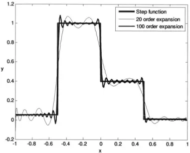
The first example is a step function with 4 piecewise constant values within each domain given in Figure 3.1. Assume we know the exact step function f(x). In order to
reconstruct it using continuous (Legendre) polynomials, continuous moments are first generated as:
Fm,
J
P,, (x)f (x)dx, (3.25)where m is the expansion order. The reconstructed step function can be obtained as:
~ M
Figure 3.1 plots
f(x)
with expansion order M=20 and 100, respectively. The oscillation effects are very obvious with different expansion orders, especially near thediscontinuities. Note that in this example the variable x varies in the domain [-1,1] and thus no extra rescaling of the function f(x) is needed to generate the moments.
1.2 Step function 1 -20 order expansion -- 100 order expansion 0.8- 0.6-y 0.4-0.2 0 -0.2 ' ' I I I I i I -1 -0.8 -0.6 -0.4 -0.2 0 0.2 0.4 0.6 0.8 1 x
Figure 3.1. Expansion of a step function using continuous Legendre polynomials.
Approximating the step function by applying a
3rd (N -1)follows. First generate discrete moments as:
N-I
F = 1jfKP (K, N -1),
K=0
order discrete expansion as
where K is the discrete variable index, m is the expansion order and N=4 in this case. The exact step function can be reconstructed as:
N-1
fK = F,,P,,(K, N -1).
=o p(m, N -1)
(3.28)
The reconstructed step function
jKis shown in Figure 3.2. Note that the expansion order
is fixed at N -1 due to the definition of discrete orthogonal polynomials. The number of
expansion moments (4) is much smaller than the continuous case (20 or 100) while it
reconstructs the step function accurately with no oscillations. Furthermore, one only
needs to know the number of discretization domains (N
=
4), while the information of
where the domains start and end is not required, i.e., Xe (-1.0, -0.5), (-0.5,0.0),
(0.0,0.5), and (0.5,1.0), respectively, in this example.
0.8 0.6 0.4 0.2-0 2 Index number 3 4 5 11 0 Step' function + 3 order expansion 0 1
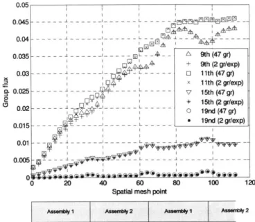
For sake of clarity on how this can be applied to nuclear reactor applications, a second example is in order. Assuming a fine group library of 47 groups, a coarse group library
of 2 energy groups can be formed (with thermal cutoff of 0.625eV, 12 and 35 fine groups within each coarse group) that is condensed from an estimated energy spectrum, as illustrated in Fig. 3.3. The system of 2 equations (assuming only energy) would correspond to the multigroup method, but the DGM method also provides 45 (34 from
group 1 and 11 from group 2) higher order equations that provide additional information about the energy spectrum, which is shown in Fig. 3.3. These additional equations are all independent of each other and only depend on the zeroth order solution.
Coarse group Energy structure
OeV
I
0.625eV
1 group
|
1 group 20MeVIFine group Energy structure
OeV
I
t
0.625eV
20MeV
12 groups | 35 groups | 'IDGM method OeV 0.625eV 20MeV
Energy structure | 1 group
I
I group |+11 order expansions +34 order expansions
Fig. 3.3. 47 group cross section condensation.
3.3. Computational results
of boiling water reactor BWR core configurations, each composed of seven fuel
assemblies. The full description of these problems, illustrated in Figure 3.4, can be found in [Rahnema 2008]. The method was tested on all four assemblies and three cores on an Intel 2.4GHz Core (TM) 2 Duo P8600 2.4 GHz PC. The current implementation is limited to discrete-ordinates, but the extension to other solution techniques of the
transport equation or diffusion equation is straightforward. It should also be noted that the 1 -D discrete-ordinate implementation includes no form of acceleration as this facilitates the comparison between methods. However, it should be noted that acceleration
techniques would most certainly reduce the computational time disparity presented in these results.
Core 1
Core 2
I[M
Core 3
Assembly 1 Assembly 2 Assembly 3 Assembly 4 Water
[
Fuel I :- Fuel il 0 Fuel + Gd M Figure 3.4. 1-D BWR core and assembly configurations.In l-D discrete ordinates, assuming isotropic scattering and applying transport cross-sections as a linear anisotropic scattering approximation, Eq. (3.23) can be written as:
+
( :rOg (X)Vig (x,pt) + ,g (x,U)y,0g (x,p)=
G () + (X)G
((3.29)
2
x).
x2 k
v
p
,
xwhere the transport cross-section moments and the perturbation term are defined in the
same way as Eqs. (3.8)-(3.11) by using transport section data instead of total
cross-section data.
3.3.1 One dimensional BWR assembly tests
The DGM method was initially tested on each of the four assemblies. It should also be
noted that for this first test case, the cross-section moments were generated with the exact
reference spectrum, thus the goal of this test is to verify the accuracy of the
approximation made in the DGM method. In this implementation, an 8 group
cross-section database serves as the "fine" group structure and is used to calculate our reference
solution. The DGM method is applied to a 1 group database with 7 order expansion
condensed from the reference solution. Both the reference and the DGM calculations are
performed using an S1
6angular approximation and the same spatial mesh. The scalar
flux is converged to 10-
5and the eigenvalue is converged to within 10-6. Reflective
boundary conditions are set on both sides. The step difference [Lewis 1993] method is
Results for assemblies 1 and 4 are given in Tables 3.1-3.3 as they give a good breath of the capabilities of the method. Assembly 4 is by far the most constraining assembly due to the high Gadolinium loading. The reported computational time for the 1 group with expansion also includes the time needed to generate the cross-section moments.
Table 3.1. Assemblies 1 and 4 eigenvalue and computational time.
Eigenvalue Ak Computational k (pcm) time (seconds) Assembly 1, 8 group 1.240588 - 0.3 Assembly 1, 1 group/exp 1.240576 1.2 0.03 Assembly 4, 8 group 0.323416 -- 0.2 Assembly 4, 1 group/exp 0.323416 0.0 0.02
Table 3.2 Assembly 1 DGM result errors.
rms (%) mre (%) err. (%)
Scalar flux 0.00035 0.00015 0.0012
Absorption rate 0.00013 0.000098 0.00020
Table 3.3 Assembly 4 DGM result errors.
rms (%) mre (%) err.(%)
Scalar flux 0.052 0.00098 0.31
As seen in Tables 3.1, 3.2 and 3.3, the DGM method gives an accurate flux solution while the computational time is much less than the fine group calculation. The values of the root mean square relative error, mean relative error, and maximum relative error of scalar flux and absorption rate of assembly 4 are larger than those of assembly 1 because of the strong heterogeneities of assembly 4 caused by the presence of Gadolinium. The mean relative error is an average error in which the relative errors are weighted by the flux values. For assembly 4, the mean relative error is much smaller than the root mean square error, which indicates that the larger errors occur in regions of very low flux (i.e., thermal groups in the Gd rich regions).
3.3.2 One dimensional BWR core tests
Now that the methodology has shown the ability to reproduce the reference flux solution, a tougher test is needed to illustrate the advantages of the DGM method for whole core calculations. A comparison is made between 47 group reference solutions for the three cores of Figure 3.4 with a 2 group DGM calculation with respective expansion orders of 34 and 11. The 47 group cross sections were generated from the HELIOS lattice
depletion code [Rahnema 2008] [Giust 2000], in which the first 35 groups are in the fast region above the thermal cutoff of 0.625eV while groups 36-47 cover the thermal energy range. Once again, a S16 angular approximation is applied and the step difference method is used for the spatial sweep. The scalar flux is converged to within 105 and the
In this calculation, the 2 group cross-sections and moments needed in the DGM method are not generated from the reference solution but from fine group assembly calculations (such as would be done in current multi-level calculations). Tables 3.4-3.6 list the flux and absorption rates, eigenvalue, and the computational time (including the calculation time needed for obtaining the cross-section moments) for cores 1 and 3. The results for
core 2 were omitted from the discussion since they fall somewhere between the results of cores 1 and 3. From Table 3.4, the computational time of the DGM method is very small compare to the fine group calculation. The eigenvalues from the DGM method are equivalent to the ones from the coarse group calculations.