Penetration of the electric and magnetic field components of Schumann resonances into the ionosphere

HAL Id: hal-00317898

https://hal.archives-ouvertes.fr/hal-00317898

Submitted on 14 Oct 2005

HAL is a multi-disciplinary open access

archive for the deposit and dissemination of

sci-entific research documents, whether they are

pub-lished or not. The documents may come from

teaching and research institutions in France or

abroad, or from public or private research centers.

L’archive ouverte pluridisciplinaire HAL, est

destinée au dépôt et à la diffusion de documents

scientifiques de niveau recherche, publiés ou non,

émanant des établissements d’enseignement et de

recherche français ou étrangers, des laboratoires

publics ou privés.

Penetration of the electric and magnetic field

components of Schumann resonances into the ionosphere

V. Grimalsky, S. Koshevaya, A. Kotsarenko, R. Perez Enriquez

To cite this version:

V. Grimalsky, S. Koshevaya, A. Kotsarenko, R. Perez Enriquez. Penetration of the electric and

mag-netic field components of Schumann resonances into the ionosphere. Annales Geophysicae, European

Geosciences Union, 2005, 23 (7), pp.2559-2564. �hal-00317898�

Annales Geophysicae, 23, 2559–2564, 2005 SRef-ID: 1432-0576/ag/2005-23-2559 © European Geosciences Union 2005

Annales

Geophysicae

Penetration of the electric and magnetic field components of

Schumann resonances into the ionosphere

V. Grimalsky1, S. Koshevaya2, A. Kotsarenko3, and R. Perez Enriquez3

1_{National Institute for Astrophysics, Optics, and Electronics, Puebla 72000, Pue., Mexico}

2_{Autonomous University of Morelos, CIICAp, Av.Universidad 1001, Cuernavaca 62210, Mor., Mexico} 3_{UNAM, Center of Geoscience, Juriquilla, P.O. 1-742, Queretaro 76230, Qro, Mexico}

Received: 16 September 2004 – Revised: 21 July 2005 – Accepted: 17 August 2005 – Published: 14 October 2005

Abstract. A penetration of electric and magnetic fields of

the first global electromagnetic ELF resonance into the iono-sphere in the cavity Earth-ionoiono-sphere is investigated numeri-cally. It is shown that a penetration height for magnetic com-ponents is 2–3 times greater than for electric comcom-ponents and it depends essentially on the value of the geomagnetic field and its orientation with respect to the normal to the Earth’s surface. A penetration height for the electric field is about 50

÷70 km, and for the magnetic field it is 120÷240 km. An in-fluence of variations of the conductivity of the ionosphere at the daytime and nighttime and under different solar activity on a penetration of the fields of the first Schumann resonance has been investigated.

Keywords. Electromagnetics (Guided waves) – Ionosphere

(Ionosphere-atmosphere interactions; Wave propagation)

1 Introduction

Schumann (global) electromagnetic (EM) resonances in the cavity Earth – ionosphere play an important role in the litho-sphere – atmolitho-sphere – ionolitho-sphere – magnetolitho-sphere cou-pling (Hayakawa, 1999; Bliokh et al., 1980; Nickolaenko and Hayakawa, 2002; Nickolaenko, 1997). A very rough approximation to describe the properties of the Schumann resonances is an assumption of the ideal conductivity of both the Earth’s surface and of the ionosphere E-layer. Such an approximation gives a possibility to estimate the values of the resonant frequencies (8 Hz, 14 Hz, 20 Hz, and 26 Hz). Some specifications were put forward by means of the res-onator perturbation theory (Bliokh et al., 1980; Nickolaenko and Hayakawa, 2002; Nickolaenko, 1997; Vainshtein, 1988; Sentman, 1995), where a formalism of the tensor surface impedance of the ionosphere plasma was applied. Such a theory gives a possibility to estimate the quality factor of

Correspondence to: V. Grimalsky

(vgrim@inaoep.mx)

the resonances (about 5) and to investigate an excitation of the Schumann resonator by external current sources (atmo-spheric electricity). An excitation of Schumann resonances due to thunderstorm activity has been investigated in the pa-pers (F¨ullekrug and Constable, 2000; F¨ullekrug and Reis-ing, 1998; Mushtak and Williams, 2002). Also, there are some papers devoted to a penetration of electric and mag-netic fields of the Schumann resonances into the lower iono-sphere, where an exponential (or more complicated) approx-imation of the isotropic conductivity (and, therefore, effec-tive permittivity) of the ionosphere plasma was used (Nick-olaenko and Hayakawa, 2002; Sentman, 1995). When ne-glecting an influence of the geomagnetic field, a penetration height for the electric field was estimated as 50÷70 km, and for the magnetic field it was about 80÷100 km. The mod-ification of the properties of resonance modes due to solar activity has been observed and investigated within an ap-proximation of the isotropic conductivity of the ionosphere (Roldugin, 2003). Also, the dissipation of Schumann modes has been estimated from the approximation of isotropic iono-sphere (Sentman, 1983). Note that an essential influence of the geomagnetic field on a penetration of extremely low frequency (ELF) electromagnetic fields into the ionosphere was mentioned in the early survey (Madden and Thompson, 1965). Moreover, some authors, who used an isotropic ap-proximation, mentioned an importance of the anisotropy of the conductivity of the ionosphere (Sentman, 1983; Mushtak and Williams, 2002).

The vertical profile of the conductivity of the ionosphere is not ideally sharp; its characteristic scale of variation is about 10÷30 km. A strong anisotropy of conductivity of the ionosphere, due to the presence of the geomagnetic field, be-comes essential at the heights of 70÷80 km and more (Mad-den and Thompson, 1965; Rich and Basu, 1985; Al’pert, 1972). Thus, a modification of the vertical profile of the anisotropic conductivity of the lower ionosphere, due to various processes, may lead to a change in properties of the global resonance modes. It is clear that electric and

2560 V. Grimalsky et al.: Penetration of the electric and magnetic field components of Schumann resonances 1

O

Earth

Atmosphere

Ionosphere

_z

H

₀

x

Θ

Φ

y

z’

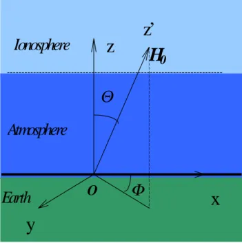
Fig.1. Geometry of the problem. (XYZ) are local coordinates.

Fig. 1. Geometry of the problem. (XYZ) are local coordinates.

magnetic components of the Schumann modes possess dif-ferent vertical distributions. But it is important to know more exactly about the difference between the corresponding pen-etration heights in the presence of the geomagnetic field.

In this paper, the vertical profiles of the electric and mag-netic fields of the first global Schumann resonance in the cavity Earth – ionosphere are investigated numerically in the cases of various vertical profiles of the electron concentra-tion of the ionosphere. The anisotropy of conductivity due to the presence of the geomagnetic field is taken into ac-count. It is shown that the horizontal magnetic components of the resonance mode can penetrate highly into the E-layer of the ionosphere and even into the F-layer. The penetration height depends on the value and orientation of the local geo-magnetic field; it is about 50÷70 km for electric components and 120÷240 km for magnetic components. For that reason, variations of the conductivity of the ionosphere D-layer may lead to essential changes in vertical profiles of both electric and magnetic components of the modes. Correspondingly, variations in the conductivity of the ionosphere E-layer may lead to changes in the vertical profiles of the magnetic com-ponents.

2 Basic equations

The global resonances in the cavity Earth – ionosphere pos-sess the resonant frequencies in the ELF range. The lowest (fundamental) frequency is about 8 Hz (Bliokh et al., 1980; Nickolaenko and Hayakawa, 2002; Nickolaenko, 1997). Due to a global character, a distribution along the Earth’s sur-face is smooth, and a characteristic scale is the Earth’s ra-dius RE=6400 km. The vertical scale of the field

distribu-tion depends on the profile of the ionosphere and it is about 10÷30 km. Thus, these scales differ from each other very essentially. This gives a possibility to consider the problem of the penetration of the EM components of the resonance mode into the ionosphere, approximately within the assump-tions that the Earth’s surface is locally plane and a horizontal dependence of EM components is the same with a change in the vertical coordinate.

Let us estimate an applicability of the plane approximation of the Earth’s surface. A deviation of the tangential line from the curved Earth’s surface is zs=L2x/(2RE)at the horizon-tal distance Lx. The parameter Lx describes the horizontal scale where the ionosphere can be assumed as vertically non-uniform only. Let us choose the value Lx=400 km, which is twice as large as the possible height of a penetration of magnetic fields of the global resonances into the ionosphere. Here, zs≈12 km. Therefore, zs is smaller than a characteris-tic vercharacteris-tical scale of the ionosphere (20÷30 km), and a cur-vature of the Earth’s surface may be considered as a per-turbation. A dependence of the distributions of horizontal components of the magnetic field of the global Schumann resonances on the local height of the ionosphere D-layer was confirmed experimentally (Sentman and Fraser, 1991).

Let us denote the local vertical axis as OZ, horizontal axes are OX and OY (see Fig. 1), and assume that the horizon-tal axes are chosen so that the local dependence of the mode components in the horizontal plane is ∼exp(ikxx). A tempo-ral dependence is ∼exp(iωt), where ω is an angular resonant frequency, which is generally complex, due to the damping of the resonant mode. But, to consider the vertical profile of the mode, it is necessary to use only the real part of the res-onant frequency in the expressions of the tensor of dielectric permittivity (Vainshtein, 1988). Note that simulations with the resonant frequency including the image part (within 20% of the real part) do not change the results essentially.

The components of a dielectric tensor in the coordinate frame connected with the direction of the geomagnetic field take a form: ˆ ε0(ω, z) =   ε1 εh 0 −εh ε1 0 0 0 ε3   ; ε1=1 − ω2_pe(ω−iνe) ω((ω−iνe)2_−ω2 H e) − ω 2 pi(ω−iνi) ω((ω−iνi)2−ω2H i) ; ε3=1 − ω2_pe ω(ω−iνe) − ω2_pi ω(ω−iνi); εh=i( ω2 peωH e ω((ω−iνe)2_−ω2 H e) − ω 2 piωH i ω((ω−iνi)2_−ω2 H i) ); ω2_pe= 4π e2n0 me , ω 2 pi= 4π e2_n 0 mi , ωH e = eH0 mec, ωH i= eH0 mic.

Here n0is the electron concentration; νe,i are collision fre-quencies for electrons and ions, respectively; me,i are their masses; ωpe,i and ωH e,i are corresponding plasma and cy-clotron frequencies (Nickolaenko and Hayakawa, 2002).

V. Grimalsky et al.: Penetration of the electric and magnetic field components of Schumann resonances 2561 The set of Maxwell’s equations for the electric (Ex,y,z)

and magnetic (Hx,y,z) components of the mode takes the form: ∂2Ex ∂z2 −ikx∂E_∂zz +k20Dx =0; ∂2Ey ∂z2 −kx2Ey+k₀2Dy=0; ikx∂Ex_∂z +kx2Ez−k02Dz=0; Dj =εj l(ω, z)El;k0=ω/c;E ∼ exp(ikxx). (1)

Here εj l (ω,z) are the components of the tensor of the dielectric permittivity, ε∧(ω,z), of the atmosphere and the ionosphere in the coordinate frame (XY Z); Djare the com-ponents of the electric induction vector. The comcom-ponents εj l depend essentially on the vertical coordinate z and weakly on the horizontal coordinates x, y. An absolute system of units is used here, where the units for the electric and magnetic fields are the same. It is possible to express all the components of the mode through Dz and Ey and to obtain the coupled equations for them:

d dz( ε₃₃ 1 dDz dz ) + ikx d dz( ε₁₃ 1Dz) + ikx ε₃₁ 1 dDz dz −ikx_dzd(e1Ey) + (k 2 0−kx2 ε₁₁ 1)Dz−k 2 xe3Ey=0; d2Ey dz2 − ik2 0 kxe4 dDz dz −k02e2Dz+ +(k₀2ε˜22−kx2)Ey=0; (2) Ex=_kxi ε₃₃ 1 dDz dz − ε₁₃ 1Dz+e1Ey;Hx= − i k0 dEy dz; Ez= −_ki x ε₃₁ 1 dDz dz + ε₁₁ 1Dz+e3Ey; Hy =_kk0 xDz;Hz = − kx k0Ey; (3)

The following notations are used:

e₁ = 1 1(ε13ε32−ε12ε33); e2 = 1 1(ε21ε13−ε11ε23); e₃ = 1 1(ε31ε12−ε11ε32); e4 = 1 1(ε23ε31−ε21ε33); 1 = ε₁₁ε₃₃−ε₁₃ε₃₁;ε˜22=ε22+ε21e1+ε23e3.

The Earth’s surface is assumed to be ideally conductive, therefore, the boundary conditions are: Ey(z=0)=0, Dz (z=0)=Dz0=1; Ey(z=Lzm)=0, Dz(z=Lzm)=0 in the highly conductive F-layer of the ionosphere. The results do not depend on the choice of the upper boundary Lzm, when Lzm>250 km. The problem is to investigate the vertical pro-files of all the components of the first Schumann resonance mode.

The value of the resonant frequency of the lowest EM Schumann mode has been chosen as f ≈8 Hz (ω=50 s−1), known from experimental data (Bliokh et al., 1980; Nick-olaenko, 1997). A horizontal distribution of the mode is de-termined by the parameter kx≈R−E1, and it is approximately equal to k0=ω/c. Small deviations (up to 30%) from the

val-ues of ω and kx above do not change the main qualitative results of the paper.

2

a)

b)

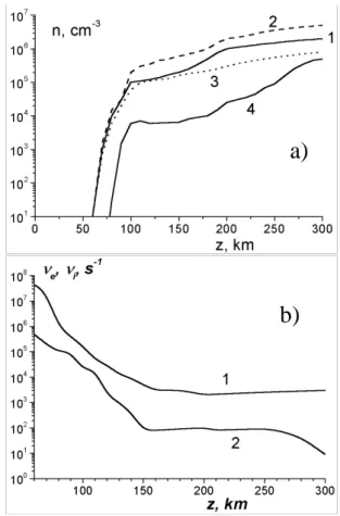
Fig.2. Part (a). Vertical dependence of the concentration of electrons used in the

simulations. Curve 1 is at the daytime (normal solar activity), curve 2 is at the daytime

(maximum solar activity), curve 3 is at the daytime (minimal solar activity), curve 4 is at

the nighttime. Part (b). Vertical dependencies of electron (curve 1) and ion (curve 2)

collision frequencies used in simulations.

2

a)

b)

Fig.2. Part (a). Vertical dependence of the concentration of electrons used in the

simulations. Curve 1 is at the daytime (normal solar activity), curve 2 is at the daytime

(maximum solar activity), curve 3 is at the daytime (minimal solar activity), curve 4 is at

the nighttime. Part (b). Vertical dependencies of electron (curve 1) and ion (curve 2)

collision frequencies used in simulations.

Fig. 2. Part (a). Vertical dependence of the concentration of

elec-trons used in the simulations. Curve 1 is at the daytime (normal solar activity), curve 2 is at the daytime (maximum solar activity), curve 3 is at the daytime (minimal solar activity), curve 4 is at the nighttime. Part (b). Vertical dependencies of electron (curve 1) and ion (curve 2) collision frequencies used in the simulations.

3 Numerical simulations

Numerical simulations have been provided by means of a fi-nite difference approximation of Eq. (2). The obtained three-diagonal matrix linear equations have been solved by the matrix factorization method. The steps of the calculations are 50 m–3 m. The vertical profiles of the concentration of electrons used in the simulations are given in Fig. 2. The data on the concentrations of electrons, collision frequencies, and average molar masses have been taken from Rich and Basu (1985); Al’pert (1972). One can see that there exists an essential difference between the values at the daytime un-der different solar activity and at the nighttime. The vertical profiles of the absolute values of the components of the com-plex dielectric permittivity |ε1,3,h| in the coordinate frame,

connected with the geomagnetic field H0, are presented in

Fig. 3 (daytime, normal solar activity). In the simulations, the value of the electron cyclotron frequency has been taken as ωH e=6·106s−1(H0=0.35 Oe). Note that the minimal

ver-tical scale of change in the components of the dielectric per-mittivity tensor is 1 km.

2562 V. Grimalsky et al.: Penetration of the electric and magnetic field components of Schumann resonances 3

a)

b)

Fig.3. Vertical dependencies of the absolute values of components of complex tensor of

dielectric permittivity of atmosphere and ionosphere at

ω

= 50 s

used in simulations

(daytime, normal solar activity) (a). The detailed dependence for the heights 70 ÷ 110

km (b).

3

a)

b)

Fig.3. Vertical dependencies of the absolute values of components of complex tensor of

dielectric permittivity of atmosphere and ionosphere at

ω

= 50 s

used in simulations

(daytime, normal solar activity) (a). The detailed dependence for the heights 70

÷

110

km (b).

Fig. 3. Vertical dependencies of the absolute values of components

of complex tensor of dielectric permittivity of atmosphere and iono-sphere at ω=50 s−1used in the simulations (daytime, normal solar activity) (a). The detailed dependence for the heights 70÷110 km

(b).

4

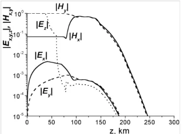
Fig.4. The dependencies of components |Ex,y,z| and |Hx,y| on the vertical coordinate z

under the inclination of the geomagnetic field Θ = 30º (daytime, normal solar activity).

Fig. 4. The dependencies of components |Ex,y,z|and |Hx,y |on

the vertical coordinate z under the inclination of the geomagnetic field 2=30◦(daytime, normal solar activity).

5

Fig.5. A dependence of components |Ex,y,z| and |Hx,y| on the vertical coordinate z in the

absence of geomagnetic field H0 = 0 (daytime, normal solar activity).

Fig. 5. A dependence of components |Ex,y,z |and |Hx,y|on the

vertical coordinate z in the absence of geomagnetic field H0=0

(daytime, normal solar activity).

Vertical distributions of electric and magnetic field com-ponents of the mode have been calculated under various ori-entations of the geomagnetic field H0, with respect to the

vertical axis OZ (angle 2) and of the plane (OZ, H0)with respect to the OX axis (angle 8), see Fig. 1. A penetration of the magnetic components Hx,y into the ionosphere depends essentially on the inclination angle 2. A dependence of the penetration of the magnetic components on the angle 8 is unessential. In Fig. 4, dependencies of |Ex,y,z|, |Hx,y|on the vertical coordinate z are given for the value of the inclination angle 2=30◦and for 8=30◦. The normal daytime conditions are assumed here (Rich and Basu, 1985). The vertical mag-netic component Hzis quite small: |Hz|≈|Ey|.

At the Earth’s surface the components Ez and Hy pos-sess the greatest values, as well-known earlier (Bliokh et al., 1980; Nickolaenko and Hayakawa, 2002). But the vertical distributions of the electric and magnetic components differ from each other. Moreover, the presence of the geomagnetic field changes essentially the vertical distributions of the hori-zontal magnetic field components, as shown in Fig. 5, where the vertical distributions of the field components are given in the absence of the geomagnetic field, to compare with Fig. 4. The data of Fig. 5 coincide with the results of the survey (Sentman, 1995) and the papers cited there. Indepen-dent of the presence or absence of the geomagnetic field, at the heights z>50 km, Ezdecreases quickly and it becomes of the same order as the Ex and Ey components. The electric field of the mode does not penetrate highly into the iono-sphere, as was known earlier (Sentman, 1995). Moreover, the dependence of Ez(z)coincides with the dependence ob-tained in the paper by Sentman (1990), where a two-scale exponential approximation of isotropic conductivity of the ionosphere was used. But the magnetic field components

Hx,y can penetrate into the E-layer of the ionosphere up to the heights z≈150 km, (compare Figs. 4 and 5). Under the oblique direction of the geomagnetic field, a penetration of magnetic components becomes weaker, but it also exceeds

V. Grimalsky et al.: Penetration of the electric and magnetic field components of Schumann resonances 2563

6

a)

b)

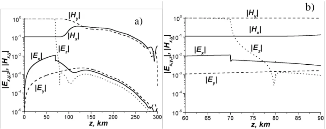
Fig.6. A dependence of components |Ex,y,z| and |Hx,y| on the vertical coordinate z under Θ

= 30º (nighttime) (a). The detailed dependence for the heights 60 ÷ 90 km (b).

6

a)

b)

Fig.6. A dependence of components |Ex,y,z

| and |H

| on the vertical coordinate z under

Θ

= 30º (nighttime) (a). The detailed dependence for the heights 60 ÷ 90 km (b).

Fig. 6. A dependence of components |Ex,y,z|and |Hx,y|on the vertical coordinate z under 2=30◦ (nighttime) (a). The detailed dependence

for the heights 60÷90 km (b).

7

a)

b)

c)

d)

Fig. 7. Dependencies of the penetration heights of the components Hx,y of the Schumann

resonance on the inclination angle Θ of the geomagnetic field. Part a) is for the daytime

(normal solar activity); b) is for daytime (maximum solar activity); c) is for the daytime

(minimum solar activity); d) is for the nighttime. Curve 1 is the penetration height for

H

height for Ez component is 56 km. For the nighttime, it is 71 km.

7

a)

b)

c)

d)

Fig. 7. Dependencies of the penetration heights of the components H

of the Schumann

resonance on the inclination angle

Θ

of the geomagnetic field. Part a) is for the daytime

(normal solar activity); b) is for daytime (maximum solar activity); c) is for the daytime

(minimum solar activity); d) is for the nighttime. Curve 1 is the penetration height for

H

component, 2 is the penetration height for H

. For the daytime, the penetration

height for E

component is 56 km. For the nighttime, it is 71 km.

7

a)

b)

c)

d)

Fig. 7. Dependencies of the penetration heights of the components Hx,y of the Schumann

resonance on the inclination angle

Θ

of the geomagnetic field. Part a) is for the daytime

(normal solar activity); b) is for daytime (maximum solar activity); c) is for the daytime

(minimum solar activity); d) is for the nighttime. Curve 1 is the penetration height for

H

height for Ez component is 56 km. For the nighttime, it is 71 km.

7

a)

b)

c)

d)

Fig. 7. Dependencies of the penetration heights of the components Hx,y of the Schumann

resonance on the inclination angle

Θ

of the geomagnetic field. Part a) is for the daytime

(normal solar activity); b) is for daytime (maximum solar activity); c) is for the daytime

(minimum solar activity); d) is for the nighttime. Curve 1 is the penetration height for

H

height for Ez component is 56 km. For the nighttime, it is 71 km.

Fig. 7. Dependencies of the penetration heights of the components Hx,y of the Schumann resonance on the inclination angle 2 of the

geomagnetic field. Part (a) is for the daytime (normal solar activity); (b) is for daytime (maximum solar activity); (c) is for the daytime (minimum solar activity); (d) is for the nighttime. Curve 1 is the penetration height for Hxcomponent; curve 2 is the penetration height for

Hy. For the daytime, the penetration height for the Ezcomponent is 56 km. For the nighttime, it is 71 km.

the values obtained in the absence of the geomagnetic field. At the heights z>50 km the components Ex,yare of the same order as Ez, also Hx is of the same order as Hy. Therefore, perturbations of the conductivity of the ionosphere D-layer may change the vertical profiles of both electric and magnetic components of the Schumann resonances; the variations of the conductivity of the ionosphere E-layer may lead to the changes in the vertical profiles of magnetic components.

In Fig. 6, the vertical distributions of the field components are presented at the nighttime (normal solar activity). The inclination angle is also 2=30◦. The use of more smooth profiles of the electron concentration n(z) at the heights 60÷110 km does not change the vertical dependencies of the magnetic components Hx, Hybut only leads to smoother de-pendencies of Exand Eycomponents of the electric field.

2564 V. Grimalsky et al.: Penetration of the electric and magnetic field components of Schumann resonances In Fig. 7 the dependencies of the penetration heights on

the inclination angle 2 are given for the normal solar ac-tivity, maximal and minimum solar activity (daytime), and the normal solar activity (nighttime). The penetration height is estimated as the value of the vertical coordinate z, where

|Hx|or |Hy|is 0.1|Hy(z=0)|. One can see some dependence of a penetration height of horizontal magnetic field compo-nents on the variations of the profiles of the electron concen-tration at the daytime (Figs. 7a,b,c). An essential difference is between the dependencies of the horizontal magnetic field components on the coordinate z at the daytime and the night-time. The last fact may be explained by the absence of the ionosphere D-layer at the nighttime (Rich and Basu, 1985; Al’pert, 1972). Thus, the horizontal magnetic components of the Schumann resonance possess, at the same time, dif-ferent penetration heights at difdif-ferent places on the Earth. For the daytime, the penetration height for Ezcomponent is 55 km, independent of the solar activity; for the nighttime, it is 70 km.

The maximal penetration takes place at 2≈0◦, namely, under a vertical direction of the geomagnetic field. It is in-teresting that at the nighttime, the horizontal magnetic com-ponents penetrate deeply into the F-layer (see Figs. 6 and Fig. 7d) This fact may lead to additional dissipation of the Schumann resonances.

To estimate the influence of the curvature of the Earth’s surface on the penetration of the magnetic field components into the ionosphere, the spherical geometry has also been in-vestigated. A simple model situation has been considered when the geomagnetic field is directed vertically upwards and is constant. The results of the simulations have con-firmed the possibility of the penetration of horizontal compo-nents of the magnetic field up to the heights of 120÷200 km.

4 Conclusions

The simulations of the penetration of the electric and mag-netic components of the first Schumann resonance mode into the ionosphere in the cavity Earth – ionosphere have been made in the case of possible daytime and nighttime variations of the conductivity in the ionosphere D- and E-layers. The magnetic components can penetrate into the E-layer of the ionosphere up to the heights z=150÷240 km, with a depen-dence on the local orientation of the geomagnetic field with respect to the vertical axis. Therefore, variations of the con-centration of electrons in the D-layer (z∼60 km) may change the profiles of electric components of the global Schumann resonances; perturbations of the E-layer (z∼100÷150 km), due to magnetosphere-ionosphere coupling, may change the profiles of the magnetic components of the global Schumann resonances.

The total energy of the EM resonant mode includes both electric and magnetic parts. Because the magnetic field of the Schumann resonance penetrates up to the heights 150÷240 km in the presence of the geomagnetic field, it is necessary to take into account this fact when calculating

the excitation of the resonant mode by thunderstorm activ-ity. The strong anisotropy of the effective dielectric permit-tivity at the heights z≥70 km is also important for estima-tions of quality factors of Schumann resonance modes and for determining the regions of maximal dissipation of ELF electromagnetic waves under the propagation in the Earth-ionosphere cavity.

Acknowledgements. Topical Editor M. Lester thanks two referees

for their help in evaluating this paper.

References

Al’pert, I. L.: Radio Wave Propagation and the Ionosphere. Nauka, Moscow, 1972.

Bliokh, P. V., Nickolaenko, A. P., and Filippov, Yu. F.: Schu-mann Resonances in the Earth-Ionosheric Cavity. Peter Peregri-nus, London, 1980.

F¨ullekrug, M. and Constable, S.: Global triangulation of intense lightning discharges, Geophys. Res. Lett., 27, 333–336, 2000. F¨ullekrug, M. and Reising, S. C.: Excitation of Earth-Ionosphere

cavity resonances by sprite-associated lightning flashes, Geo-phys. Res. Lett., 25, 4145–4148, 1998.

Hayakawa, M.: Atmospheric and Ionospheric EM Phenomena. Ter-raPub, Tokyo, 1999.

Madden, T. and Thompson, W.: Low frequency electromagnetic os-cillations of the Earth-ionosphere cavity, Reviews of Geophysics, 3, 211–256, 1965.

Mushtak, V. C. and Williams, E. R.: ELF propagation parameters for uniform models of the Earth – Ionosphere waveguide, J. At-mos. S.-P., 64, 1989–2001, 2002.

Nickolaenko, A. P.: Modern aspects of Schumann resonance stud-ies, J. Atmos. S.-P., 59, 805–817, 1997.

Nickolaenko, A. P. and Hayakawa, M.: Resonances in the Earth – Ionosphere Cavity. Kluwer, Dordrecht, 2002.

Rich, F. J. and Basu, Su.: Ionospheric Physics, Handbook of physics and Space Environment, Chapter 9. Air Force Geo-physics Lab., US Air Force, 1985.

Roldugin, V. C., Maltsev, Y. P., Vasiljev, A. N., et al.: Changes of Schumann resonance parameters during the solar proton

event of 14 July 2000: J. of Geophys. Res., A108(1103),

doi:1029/2002JA009495, 2003.

Sentman, D. D.: Schumann resonance effects of electrical conduc-tivity perturbations in an exponential atmospheric/ionospheric profile, J. Atmospheric and Terrestrial Phys., 45, 1, 55–65, 1983. Sentman, D. D.: Approximate Schumann resonance parameters for a two-scale-height ionosphere, J. Atmospheric and Terrestrial Phys., 52, 1, 35–43, 1990.

Sentman, D. D. and Fraser, B. J.: Simultaneous observations of Schumann resonances in California and Australia: evidence for intensity modulation by the local height of the D region, J. Geo-phys. Res., A96(9), 15 973–15 982, 1991.

Sentman, D. D.: Schumann Resonances, Handbook of Atmospheric Electrodynamics, 1, CRC Press, Boca Raton, CA, 1995. Vainshtein, L. A.: Electromagnetic Waves. Moscow, Radio i Svyaz,