Model results for the ionospheric lower transition height over mid-latitude

HAL Id: hal-00317420

https://hal.archives-ouvertes.fr/hal-00317420

Submitted on 14 Jun 2004

HAL is a multi-disciplinary open access

archive for the deposit and dissemination of

sci-entific research documents, whether they are

pub-lished or not. The documents may come from

teaching and research institutions in France or

abroad, or from public or private research centers.

L’archive ouverte pluridisciplinaire HAL, est

destinée au dépôt et à la diffusion de documents

scientifiques de niveau recherche, publiés ou non,

émanant des établissements d’enseignement et de

recherche français ou étrangers, des laboratoires

publics ou privés.

Model results for the ionospheric lower transition height

over mid-latitude

J. Lei, L. Liu, W. Wan, S.-R. Zhang

To cite this version:

J. Lei, L. Liu, W. Wan, S.-R. Zhang. Model results for the ionospheric lower transition height over

mid-latitude. Annales Geophysicae, European Geosciences Union, 2004, 22 (6), pp.2037-2045.

�hal-00317420�

SRef-ID: 1432-0576/ag/2004-22-2037 © European Geosciences Union 2004

Annales

Geophysicae

Model results for the ionospheric lower transition height over

mid-latitude

J. Lei1, 2_{, L. Liu}1_{, W. Wan}1_{, and S.-R. Zhang}3

1_{Institute of Geology and Geophysics, Chinese Academy of Sciences, Beijing 100029, China}

2_{Wuhan Ionospheric Observatory, Wuhan Institute of Physics and Mathematics, Chinese Academy of Sciences, Wuhan}

430071, China

3_{Haystack Observatory, Massachusetts Institute of Technology, Westford, Massachusetts, USA}

Received: 7 November 2003 – Revised: 25 February 2004 – Accepted: 8 March 2004 – Published: 14 June 2004

Abstract. Theoretical calculations of the ionospheric lower transition height (LTH), a level of equal O+ and molecu-lar ion densities, were performed and compared with em-pirical models by Zhang et al. (1996). This paper repre-sents a substantial extension of the prior work by including the AE-C data of ion composition analysis and by detailed quantitative studies of the LTH simulation, and by creating a new LTH empirical model based on our simulations. Re-sults show that: (1) the calculated LTH, in general, is low-est near 11–13 LT and reaches the diurnal maximum after midnight (about 01∼02 LT). The local time asymmetry be-comes more evident in summer, when the time of minimum shifts to 16 LT. (2) The simulated LTH presents a dominant, semiannual variation during nighttime, and a pronounced an-nual variation during daytime. (3) The simulated LTH in-creases with solar activity at night and dein-creases by day, while the standard IRI option has an opposite tendency at night in summer and equinox. Therefore, the day-night dif-ference of simulated LTH significantly increases with solar activity. (4) Both daytime and nighttime LTHs, tend to in-crease with the increasing geomagnetic activity Ap index,

with a mean slope about 0.1455 km per Apunit. (5) The

di-urnal variation of LTH is found to be more than 20 km, which is much larger than the seasonal variation under F107=100 and Ap=10. Thus, the diurnal and solar activity variations

of LTH are more pronounced than its seasonal and magnetic activity variations.

Key words. Ionosphere (ion chemistry and composition; modeling and forecasting; middle-latitude ionosphere)

1 Introduction

The lower transition height (LTH) is an important parameter representing the level where the concentrations of atomic and molecular ions are equal. As is known, deriving the plasma parameters in the F1-region from the incoherent scatter radar Correspondence to: J. Lei

(leijh@wipm.ac.cn)

(ISR) spectrum depends on the assumption of the ion com-position profile (e.g. Pavlov and Buonsanto, 1998; Schlesier and Buonsanto, 1999; Pavlov et al., 1999). On the other hand, the lower transition height can be used as an anchor point for the empirical model of the ionospheric ion compo-sition profile by the International Reference Ionosphere (IRI) (Bilitza, 1990a, 1991). Therefore, a better understanding of this characteristic height will be very helpful for the analysis of ISR data and will open up the possibility of improving the IRI ion composition representation.

Several studies have investigated the variation of the ion composition which is closely related to the LTH. Oliver (1975) studied the ion composition in the F1-region with rockets and satellites data, and developed an empirical formulation for the lower transition height (Bilitza, 1990a), which involved the zenith angle, seasonal, annual and semi-annual variations, but did not include the solar flux and mag-netic activity variations. Danilov and Yaichinikov (1985) constructed an ion composition model for IRI (Bilitza, 1990a) based on the rockets data, which yields, however, a quite small day-night difference of LTH (Zhang et al., 1996). Hoegy et al. (1991) compared ion compositions measured by a number of satellites with empirical/theoretical mod-els and revealed some outstanding differences. Danilov and Simirnova (1995) produced a new ion composition model that updated the Danilov and Yaichinikov (1985) model and was used in the IRI2000 model (Bilitza, 2001). Also, the ion composition information can be deduced from ISR experi-ential data (Lathuillere and Pibaret, 1992; Cabrit and Kof-man, 1996; Litvine et al., 1998), although the inversion anal-ysis is mainly implemented for the EISCAT scatter radar and strongly depends on the data resolution and geophysical con-ditions. Because of spare observed data for the ion composi-tion in the F1-region, theoretical models can help understand the variations in the ion composition parameters and fill the data gap. Zhang et al. (1996) compared the calculated LTH with IRI and Oliver’s model, and obtained some meaningful results, while they did not carry out quantitative studies of this characteristic height.

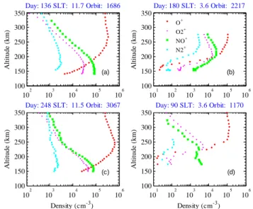
2038 J. Lei et al.: Model results for the ionospheric lower transition height over mid-latitude 102 103 104 105 106 100 150 200 250 300 350 Day: 136 SLT: 11.7 Orbit: 1686 A ltitu de ( k m) (a) 101 102 103 104 105 106 100 150 200 250 300 350 Day: 180 SLT: 3.6 Orbit: 2217 A ltitu de ( k m) (b) O+ O2+ NO+ N2+ 102 103 104 105 106 100 150 200 250 300 350 Day: 248 SLT: 11.5 Orbit: 3067 Density (cm-3) A ltitu de ( k m) (c) 101 102 103 104 105 106 100 150 200 250 300 350 Day: 90 SLT: 3.6 Orbit: 1170 Density (cm-3) A ltitu de ( k m) (d)

Figure 1. Altitude profiles of ion composition obtained from Atmosphere Explorer-C.

Fig. 1. Altitude profiles of ion composition obtained from

Atmo-sphere Explorer-C.

The aim of this study is to investigate the diurnal, seasonal, annual and semiannual variations of LTH. We will focus on the quantitative variations of LTH with solar flux F107 and magnetic activity Ap indices to extend the work of Zhang

et al. (1996). Furthermore, an empirical model is developed to depict the variation in LTH at mid-latitude based on our calculations. First, we give a description of the ionospheric model in Sect. 2, and then in Sect. 3 present simulated results and also a comparison with LTH from the AE-C ion compo-sition data. Finally, the discussions and summary are made.

2 Ionospheric model

A one-dimensional theoretical model has been developed for the mid-latitude ionosphere over the altitude range of 100– 600 km. It solves the equations of mass continuity and mo-tion for O+. Ion densities for O+₂, NO+, and N+₂ are cal-culated under the assumption of photochemical equilibrium. The solar flux EUVAC model (Richards et al., 1994) is used to define the EUV flux, and the absorption and ionization cross sections are taken from Richards et al. (1994). Mean-while, the scheme for calculating the secondary ionizations is taken from Titheridge (1996). The nighttime EUV fluxes are based on the work of Strobel et al. (1974), and the night-time photoionization cross sections are obtained from Huba et al. (2000).

We include 21 chemical reactions for O+(4S), O+(2D), O+(2P), O+₂, N+₂, and NO+, which are listed in Table 1. The scheme of chemical reactions is somewhat similar to the model of Pavlov and Foster (2001) and Pavlov (2003) in terms of the reaction rates for stable and meta-stable ions. As emphasized by Pavlov et al. (1999, and references therein), the vibrationally excited N2and O2have significant effects

on the O+loss rate. The model includes the O+(4S)+N2(v) 1010 1011 1012 1013 100 200 300 400 500 Density (m-3) A ltitu d e ( k m ) O+ NO+ O₂+ Millstone Hill 12:00 LT 0 0.5 1 100 200 300 400 500 O+/Ne Simulation Millstone Model

Figure 2. Example of the comparison between the observed electron profile (symbol ‘+’) and the model (solid line) on 27 September 2000, and O+_{, O}

2+, and NO+ concentrations are also presented

(left panel). In right panel, calculated O+/Ne are compared to the Millstone Hill standard ion-composition model. 0 4 8 12 16 20 24 160 180 200 220 240 260 280 300 LT (h) A ltitud e ( k m) Spring calculation D&S model standard IRI 0 4 8 12 16 20 24 160 180 200 220 240 260 280 300 LT (h) A ltitud e ( k m) Summer calculation D&S model standard IRI 0 4 8 12 16 20 24 160 180 200 220 240 260 280 300 LT (h) A ltitu de ( k m) Autumn calculation D&S model standard IRI 0 4 8 12 16 20 24 160 180 200 220 240 260 280 300 LT (h) A ltitu de ( k m) Winter calculation D&S model standard IRI

Figure 3. Diurnal variation of the lower transition height as given by the simulated results, the standard IRI and D&S model (Danilov and Simirnova, 1995) for four seasons under F107=100 and Ap=10.

Fig. 2. Example of the comparison between the observed electron

profile (symbol “+”) and the model (solid line) on 27 September 2000, and O+, O+₂, and NO+ concentrations are also presented (left panel). In right panel, calculated O+/N e are compared to the Millstone Hill standard ion-composition model.

reaction rate measured by Schmeltekopf et al. (1968), and the reaction rate constants for the first five vibrational levels are obtained from Pavlov et al. (1999) (see Table 1). The analytical approach for the solution of the steady-state tional quanta continuity equation is used to provide the vibra-tional temperature Tvib, which can give the similar results for

NmF2and hmF2to the full solution of the vibrational quanta

continuity equation (Pavlov and Buonsanto, 1996). The rate coefficients of O+(4S)+O2(v)are given by Hierl et al. (1997)

to include the effect of O2(v).

The ion continuity equation for O+ can be solved by an implicit, time-stepping numerical method with specified boundary and initial conditions. For the lower boundary at 100 km, an assumption of photochemical equilibrium is adopted. The electron densities at the upper boundary and plasma temperatures between the boundaries are provided by a local ionospheric model (Holt et al., 2002), which was constructed from the incoherent scatter radar measurements made since 1976 over Millstone Hill. Neutral atmospheric parameters are taken from the NRLMSISE-00 model (Picone et al., 2002), and the NO density is calculated from an em-pirical model developed by Titheridge (1997). The HWM93 model (Hedin et al., 1996) is applied to specify neutral winds for our ionospheric model.

Model calculations were carried out for Millstone Hill (42.6◦_{N, 288.5}◦_{E) under a variety of solar geophysical}

con-ditions: day number of the year between 10 and 360 with an increment of 10, F107 index between 60 and 240 with an in-crement of 20, and Ap values between 10 and 210 with an

increment of 10.

3 Observations and model calculations

The purpose of the AE-C mission was to investigate the thermosphere, with an emphasis on the energy transfer and processes that govern its state (http://nssdc.gsfc.nasa.gov/ ftphelper/). A lot of collected data can be used to study in

J. Lei et al.: Model results for the ionospheric lower transition height over mid-latitude 2039 1010 1011 1012 1013 100 200 300 400 Density (m-3) A ltitu d e ( k m ) O+ NO+ O₂+ 0 0.5 1 100 200 300 400 O+/Ne Simulation Millstone Model

Figure 2. Example of the comparison between the observed electron profile (symbol ‘+’) and the model (solid line) on 27 September 2000, and O+_{, O}

2+, and NO+ concentrations are also presented

(left panel). In right panel, calculated O+_{/Ne are compared to the Millstone Hill standard}

ion-composition model. 0 4 8 12 16 20 24 160 180 200 220 240 260 280 300 LT (h) A ltitud e ( k m) Spring calculation D&S model standard IRI 0 4 8 12 16 20 24 160 180 200 220 240 260 280 300 LT (h) A ltitud e ( k m) Summer calculation D&S model standard IRI 0 4 8 12 16 20 24 160 180 200 220 240 260 280 300 LT (h) A ltitu de ( k m) Autumn calculation D&S model standard IRI 0 4 8 12 16 20 24 160 180 200 220 240 260 280 300 LT (h) A ltitu de ( k m) Winter calculation D&S model standard IRI

Figure 3. Diurnal variation of the lower transition height as given by the simulated results, the standard IRI and D&S model (Danilov and Simirnova, 1995) for four seasons under F107=100 and Ap=10.

Fig. 3. Diurnal variation of the lower transition height as given by

the simulated results, the standard IRI and D&S model (Danilov and Simirnova, 1995) for four seasons under F107=100 and Ap=10.

great detail the ionosphere and thermosphere (upper atmo-sphere) and the coupling processes between them. The AE-C satellite was initially injected into a highly elliptical orbit with an apogee near 4000 km and a perigee near 150 km, with an inclination of 67◦_{. For the first 12 months after its}

emis-sion, its perigee was periodically lowered to 137 km while its apogee decayed rapidly. The orbit was changed to a circular orbit at about 300 km and was kept in this orbit mode from March 1975 to December 1976. The satellite was then raised to about 400 km and remained in a circular orbit at this height for the rest of its lifetime. Therefore, during the low perigee period, the ion density profiles at lower F-regional altitudes can be used to determine the lower transition height (LTH) for this study. We made use of individual ion density derived from the magnetic ion mass spectrometer (MIMS) (Hoffman et al., 1973). To give comparison with our model results, we limited the AE-C ion composition data to the latitude range of 20–60◦_{, and assumed that the horizontal variation of ion}

density at middle latitudes can be negligible. Figure 1 shows the measured ion composition from the perigee to higher al-titudes from 4 orbits. The molecular ions O+₂ and NO+are the main constituents below the F1-region, while O+is the dominant species above this altitude in the F-region. The transition height from dominant molecular to atomic ions is higher during nighttime (Fig. 1b and d) than during daytime (Fig. 1a and c), and higher in summer (Fig. 1a and b) than in equinox (Fig. 1c and d).

Figure 2 shows the comparison of height profiles of the calculated electron density with the ISR observation, and the ion species on 27 September 2000 over Millstone Hill. The good agreement between the model and observed elec-tron density validates our model results. The simulated ion composition shows good agreement with the observation in Fig. 1. The transition height is around 180 km during

day-140 180 220 260 300 A ltitu de ( k m) F107=80 simulation 140 180 220 260 300 A ltitud e ( k m) D&S model 0 4 8 12 16 20 24 140 180 220 260 300 LT (h) A ltitu de ( k m) standard IRI 140 180 220 260 300 A ltitu de ( k m) F107=160 simulation 140 180 220 260 300 A ltitud e ( k m) D&S model 0 4 8 12 16 20 24 140 180 220 260 300 LT (h) A ltitu de ( k m) standard IRI

Figure 4. Seasonal effect shown by the simulated LTH and the IRI model (standard IRI and D&S model) at two solar activity levels: left panel for F107=80, and right panel for F107=160. Heavy solid lines for summer, dash lines for equinox, and light solid lines for winter.

Fig. 4. Seasonal effect shown by the simulated LTH and the IRI

model (standard IRI and D&S model) at two solar activity levels: left panel for F107=80, and right panel for F107=160. Heavy solid lines for summer, dash lines for equinox, and light solid lines for winter.

time, and rises to higher altitudes at night (see Figs. 3 and 4). The calculated O+_{/Ne ratio is very close to the}

stan-dard Millstone Hill ion composition model on this quiet day, so no correction is needed to apply to the measured Ne(h), Te(h) andTi(h). However, under disturbed days, differences in O+/Ne ratio between the model results and the standard Millstone Hill ion composition model (Schlesier and Buon-santo, 1999; Pavlov et al., 1999) are likely to occur. As a re-sult, the calculated ion compositions from ionospheric model may be used to correct the measured temperature and elec-tron density by utilizing the multiplicative factors of Wald-teufel (1971).

3.1 Diurnal and seasonal variations

Figure 3 shows the diurnal variations of the simulated LTH for four seasons against local time (LT) under F107=100 and Ap=10. The diurnal variation of LTH is, in general, similar

to that of the peak density height (hmF2), lower during the day and higher by night. Table 2 shows characteristic values of the diurnal variation of LTH, which reaches its maximum at about 01–02 LT, and its minimum at 11–13 LT for all sea-sons except during summer, where the minimum value oc-curs at 16 LT in the afternoon. The diurnal variation shows an almost identical behavior in spring and autumn, so we will use the equinox case to represent its variations in these two seasons in the afterward discussion. The LTH shows the largest day-night difference in equinox seasons and the least in summer. This behavior is not uniform with the analysis for EISCAT measurements by Litvine et al. (1998). They found that the smallest amplitude of the daily variation takes place in winter and the minimum of winter shifts to 15 LT in the af-ternoon. The difference between the two sites may be caused by the latitudinal variations suggested by Bilitza (1990a).

2040 J. Lei et al.: Model results for the ionospheric lower transition height over mid-latitude

Table 1. Chemical reactions and rates included in the ionospheric model. Teff=(miTn+mnTi)/(mi+mn)+0.329E2, where E is the electric

field perpendicular to the geomagnetic field in mV/m.

Reaction Rate Coefficient, m3s−1, or Rate, s−1 Reference

k10=1.533×10−18−5.92×10−19(Teff/300)

+8.60×10−20(Teff/300)2(300 K≤Teff≤1700 K)

O+(4S)+N2(v=0)→NO++N St. Maurice and Torr (1978) k10=2.73×10−18−1.155×10−18(Teff/300)

+1.483×10−19(Teff/300)2(1700 K<Teff<6000 K)

O+(4S)+N2(v)→NO++ N k1=P5v=1N2(v)k1v/N2 Pavlov et al. (1999) k11=k10; k12=38k10; k13=85k10; k14=220k10; k15=270k10;

O+(4S)+O2(v)→O+₂+O k2=1.7×10−17(300/Tn)0.77+8.54×10−17×exp(−3467/Tn) Hierl et al. (1997)

O+(2D)+N2→N+₂+O k3=1.5×10−16(Teff/300)0.5 Li et al. (1997), Pavlov (2003)

O+(2D)+O2→O+₂+O k4=1.3×10−16(Teff/300)0.5 Pavlov (2003)

O+(2D)+O→O+(4S)+O k5=1.0×10−16 Fox and Dalgarno (1985)

O+(2D)+e→O+(4S)+e k6=4.0×10−14(300/Te)0.5 McLaughlin and Bell (1998),

Pavlov (2003)

O+(2P)+N₂→N+₂+O k7=2.0×10−16(Teff/300)0.5 Li et al. (1997), Pavlov (2003)

O+(2P)+N₂→N++NO k₈=1.0×10−17 Rees (1989) O+(2P)+O→O+(4S)+O k9=4.0×10−16 Chang et al. (1993)

O+(2P)+e→O+(4S)+e k10=2.5×10−14(300/Te)0.5 McLaughlin and Bell (1998),

Pavlov (2003)

O+(2P)+e→O+(2D)+e k11=7.0×10−14(300/Te)0.5 McLaughlin and Bell (1998),

Pavlov (2003)

O+(2P)→O+(4S)+hv A1=0.0833 s−1 Kaufman and Sugar (1986)

O+(2P)→O+(2D)+hv A2=0.277 s−1 Kaufman and Sugar (1986)

O+₂+NO→NO++O2 k12=4.4×10−16 Lindinger et al. (1974)

O+₂+N→NO++O k13=1.2×10−16 Fehsenfeld (1977)

O+₂+e→O+O k₁₄=2.0×10−13(300/Te)0.7(Te<1200 K) Walls and Dunn (1974) k14=1.6×10−13(300/Te)0.55(Te≥1200 K) Torr et al. (1976)

N+₂+O→NO++N k15=1.4×10−16(300/Ti)0.44 McFarland et al. (1974)

N+₂+O→O+(4S)+N2 k16=9.8×10−18(300/Ti)0.23 McFarland et al. (1974)

N+₂+O2→O+2+N2 k17=5.0×10−17(300/Teff) Lindinger et al. (1974)

N+₂+e→N+N k18=1.75×10−13(300/Te)0.3 Peterson et al. (1998)

NO++e→N+O k19=4.2×10−13(300/Te)0.85 Torr et al. (1976)

Table 2. The extremum of LTH (maximum values Hmax, and

min-imum values Hmin)(km) of daily variation and its corresponding

local time (h).

Season Hmax tmax Hmin tmin

Spring 224 1.0 182 13.0 Summer 216 1.0 188 16.0 Autumn 222 1.5 184 13.0 Winter 218 1.5 178 11.0

Figure 3 also shows diurnal variations of the LTH predicted by IRI2000 under the same conditions. The standard IRI op-tion (Bilitza, 1990b) values share the same tendency with an-other option, the D&S model (Danilov and Simirnova, 1995), while the former is generally 20 km lower than the latter. In equinox, the daytime theoretical LTH is in agreement with the D&S model, while the nighttime LTH agrees better with

Table 3. Harmonic components of fitting mean, annual and

semi-annual variations of LTH according to Eq. (1). Amplitudes are in km, and phases in days.

Local time (hour) AD0 AD1 D1 AD2 D2

0:00 217 1 102 4 103 12:00 184 6 176 1 19

the standard option. In summer, the theoretical altitude is close to the standard IRI option. In winter, both IRI op-tions fail to predict the night values. The smaller day-night difference in both the IRI standard option and D&Y model (Danilov and Yaichinikov, 1985) was reported by Zhang et al. (1996). The D&S model, as an updated D&Y model, now yields larger day-night differences, whereas the latest

J. Lei et al.: Model results for the ionospheric lower transition height over mid-latitude 2041 0 4 8 12 16 20 24 140 160 180 200 220 240 260 280 300 LT (h) A ltitu d e (k m ) summer winter equinox

Figure 5. The diurnal and seasonal variation of LTH derived from Atmosphere Explorer-C.

0 40 80 120 160 200 240 280 320 360 0 4 8 12 16 20 24 Day number L o cal t im e ( h ou rs ) 214 202 194 18 2 186 210 222 214 222 198 190 18 6 18 2 210 194 202 206 214

Figure 6. Contour of the calculated LTH versus day of year and local time under F107=100 and Ap=10.

Fig. 5. The diurnal and seasonal variation of LTH derived from

Atmosphere Explorer-C.

0

4

8

12

16

20

24

140

160

180

200

220

240

260

280

LT (h)

A

ltitu

d

e

(k

m

)

summer

winter

equinox

Figure 5. The diurnal and seasonal variation of LTH derived from Atmosphere Explorer-C.

0 40 80 120 160 200 240 280 320 360 0 4 8 12 16 20 24

Day number

L

o

cal

t

im

e

(

h

ou

rs

)

Figure 6. Contour of the calculated LTH versus day of year and local time under F107=100 and

Ap=10.

Fig. 6. Contour of the calculated LTH versus day of year and local

time under F107=100 and Ap=10.

IRI still gives smaller day-night differences in winter. Litvine et al. (1998) had also found that the deduced LTH from EIS-CAT measurements showed similarities in the general trend with IRI, but still has some difference in the values and the exact behavior.

To give a more detailed pattern for the diurnal and sea-sonal variation, Fig. 4 displays the theoretical LTH and that from the two IRI options at two solar flux levels (F107=80 and 160). The simulated LTH shows a seasonal difference of about 10 km, while the IRI gives a difference of more than 40 km. During nighttime, the simulated LTH maximizes in equinox, while the IRI LTH reaches a maximum in summer. In general, both IRI options give an LTH too large in sum-mer, but too small in winter. The simulated solar flux effect on LTH is also different from that of the IRI model, which will be discussed in the next section.

The altitude profiles of ion composition derived from AE-C data in 1974 when F107 was about 80 are also used to obtain the LTH, as shown in Fig. 5 for comparisons with the model values in the left panels of Fig. 4. The simulated LTH agrees with AE-C measurements in many respects: The LTH has larger values at night than during daytime. During daytime, the LTH is highest in summer, while at night the values in equinox are larger than in summer. The seasonal difference is less than 10 km, which is much less than what IRI predicted. In addition, the diurnal maximum occurs at ∼01 LT in summer. Unfortunately, other important respects, such as the dependence of solar activity and magnetic activ-ity, can not be investigated due to the limited observations. 3.2 Annual and semiannual variation

The simulated LTH exhibits different annual and semian-nual variations at different local times as seen in Fig. 6. The LTH presents a dominant semiannual variation between 20∼05 LT, whereas it shows pronounced annual variations at other times. We can expect that the atmospheric parameters (neutral composition, neutral winds, etc.) contribute to this behavior. To investigate annual and semiannual variations in LTH, we express LTH at a given local time as three terms, which represent the average, annual and semiannual compo-nents, respectively: LTH(d, LT) = AD0+AD1cos 2π 365(d − D1) +AD2cos 4π 365(d − D2), (1)

where LT is local time, d is the day number of year, AD0

represents the average value, AD1, AD2are the annual and

semiannual amplitudes of LTH, and D1, D2 are the

corre-sponding phase to those components, in units of days. Table 3 gives the mean value, annual and semiannual amplitudes of LTH and the phase for two given local times. A dominant semiannual variation exhibits at midnight AD1=1 km and AD2=4 km, and a dominant annual variation

at 12 LT with AD1=6 km, and AD2=1 km. In all, the annual

and semiannual amplitudes are much smaller compared to the mean value AD0, and we can also conclude that the

sea-sonal variation of LTH is quite less than the diurnal variation, as discussed previously. Existed empirical models, however, tend to predict larger seasonal variations. The Oliver’s model presents an annual amplitude of 16.8 km and a semiannual amplitude of 9.4 km regardless of local time (Bilitza, 1990a). The standard IRI gives the similar variation to the Oliver’s model with an averaged annual amplitude of 19.5 km and semiannual amplitude of 7.5 km. And the D&S model pro-duces an almost identical amplitude (∼10 km) of the annual and semiannual variation of the transition height.

3.3 Solar activity dependence

Model calculations were made for various solar flux F107 values in order to simulate the solar activity dependence.

2042 J. Lei et al.: Model results for the ionospheric lower transition height over mid-latitude 50 100 150 200 250 160 200 240 280 A ltitu de ( k m) Noon summer 50 100 150 200 250 160 180 200 220 A ltitud e ( k m) _winter 50 100 150 200 250 160 180 200 220 240 Solar flux F107 A ltitu de ( k m) equinox 50 100 150 200 250 180 220 260 300 A ltitu de ( k m) summer Midnight 50 100 150 200 250 160 200 240 280 A ltitud e ( k m) winter 50 100 150 200 250 180 220 260 300 Solar flux F107 A ltitu de ( k m) equinox

Figure 7. Solar activity variation of LTH at noon (left panels) and midnight (right panels) for various seasons under Ap=10. The detail can be seen in the text.

0 4 8 12 16 20 24 -0.2 -0.1 0 0.1 0.2 0.3 LT (h) d h /d F 107 summer winter equinox

Figure 8. Variations of the gradient dh/dF107, which is the slope of a linear regression of transition height LTH to solar activity F107 values at equinox, summer and winter.

● Simulation △ D&S model 〇 Standard IRI

Fig. 7. Solar activity variation of LTH at noon (left panels) and

midnight (right panels) for various seasons under Ap=10. The detail

can be seen in the text.

50 100 150 200 250 160 200 240 280 A ltitu de ( k m) Noon summer 50 100 150 200 250 160 180 200 220 A ltitud e ( k m) _winter 50 100 150 200 250 160 180 200 220 240 Solar flux F107 A ltitu de ( k m) equinox 50 100 150 200 250 180 220 260 300 A ltitu de ( k m) summer Midnight 50 100 150 200 250 160 200 240 280 A ltitud e ( k m) winter 50 100 150 200 250 180 220 260 300 Solar flux F107 A ltitu de ( k m) equinox

Figure 7. Solar activity variation of LTH at noon (left panels) and midnight (right panels) for

various seasons under Ap=10. The detail can be seen in the text.

0 4 8 12 16 20 24 -0.2 -0.1 0 0.1 0.2 0.3 LT (h) d h /d F 107

summer

winter

equinox

Figure 8. Variations of the gradient dh/dF107, which is the slope of a linear regression of

transition height LTH to solar activity F107 values at equinox, summer and winter.

● Simulation △

D&S model

Standard IRI

Fig. 8. Variations of the gradient dh/dF107, which is the slope of

a linear regression of transition height LTH to solar activity F107 values at equinox, summer and winter.

Figure 7 shows variations of the calculated LTH and IRI val-ues with the solar flux for noon and midnight under Ap=10.

During daytime, the calculated LTH decreases with the so-lar flux and an almost linear decrease can also be seen when F107<200; a saturation of slow decrease can be seen when F107>200. At night, the calculated LTH increases with F107, and there is a good linear relationship between the sim-ulated LTH and F107. In the D&S model, the LTH decreases with F107 when F107<140 during daytime and the slopes of decrease are larger than the simulated ones, while the altitude does not vary (saturation effect) for F107>140. It should be

noted that there is no data in constructing the D&S model for the midnight sector (the zenith angle above 90◦_),

espe-cially in winter and equinoxes, therefore, we do not show the corresponding D&S model values during nighttime in Fig. 7 (right-hand panels). In standard IRI, the LTH presents abrupt changes with solar flux in summer and equinox. In winter, the LTH does not vary with F107. During daytime, the IRI model gives too large values in summer when F107<100, which can be observed in Fig. 4 and also have been revealed by Zhang et al. (1996). At night, because the standard IRI values show an opposite tendency to the simulated ones in summer and equinox, the values are larger than simulation when F107<100 and smaller when F107>100.

As discussed above, the solar activity dependence of LTH varies with local time. To further understand the diurnal vari-ations of the relvari-ationship between the simulated LTH and F107, we compute and present the gradient d(LTH)/d(F107) by a linear regression against local time shown in Fig. 8. We only use simulated data for F107 lower than 200 to com-pute the slope, because the saturation effect exists during daytime when F107>200. Results show the negative and positive slopes during daytime and nighttime, respectively. As a result, the day-night difference of LTH significantly increases with solar activity. The maximum magnitude of the slopes is about 0.1 km per F107 unit during daytime and around 0.2 km per F107 unit during nighttime. In addition, the transition time of the slope (reverse from positive to neg-ative, or vice versa) is 06 LT and 19 LT in summer, 09 LT and 18 LT in winter, 08 LT and 19 LT in equinox. It is obvi-ous that the duration of the decrease in LTH versus solar flux (negative slope) is longest (06–19 LT) in summer and short-est (09–18 LT) in winter.

3.4 Magnetic activity dependence

The simulated data allow us to analyze the effect of magnetic activity. The main feature is that the LTH generally increases with Ap (Fig. 9). The amount of increase has no obvious

seasonal variations. The LTH increases about 32 km at noon and 34 km at midnight when Ap increases from 10 to 210.

The slope d(LTH)/d(Ap) is near 0.1406 km and 0.1736 km

at noon and midnight, respectively, which is obtained with a linear regression. Figure 10 shows the deviation of the simu-lated LTH at certain Ap from that at Ap=10 to represent the

effect of magnetic activity. The mean slope of the linear fit is 0.1455 km per Apunit. Our results agree with those of

Lath-uillere and Pibaret (1992), which found that the amplitude of the magnetic activity variation of the LTH for Kp

rang-ing from 0 to 4+ is about 10 km. Litvin et al. (2000) have analyzed the ISR data over Millstone Hill and deduced the LTH from the measurements during 5–11 June 1991, a storm period. They also revealed that the LTH increased with mag-netic activity. However, their slope is somewhat larger than our simulated result.

J. Lei et al.: Model results for the ionospheric lower transition height over mid-latitude 2043

Table 4. Harmonic components of the daily variation of LTH shown

in Fig. 3. Amplitudes are in km, and phases in hours.

Season A0 A24 t24 A12 t12 A8 t8

Summer 199.3 13.4 1.51 3.5 0.70 1.0 3.49 Equinox 199.1 21.4 0.96 3.7 1.82 1.5 3.90 Winter 196.4 18.7 1.15 3.7 3.50 0.5 0.96

Table 5. Harmonic components of the slope d(LTH)/d(F107) shown in Fig. 8. Season C0 C24 φ24 C12 φ12 C8 φ8 Summer 0.010 0.179 0.187 0.055 0.534 0.008 2.985 Equinox 0.044 0.172 0.163 0.036 0.477 0.004 −0.286 Winter 0.037 0.122 0.481 0.017 0.689 0.013 −0.517 3.5 An empirical model

The simulated LTH is fitted using the following equation

LTH(t) = A0+ 3 X n=1 A24/ncos(2π t − t24/n 24/n ) +[C0+ 3 X n=1 C24/ncos(2π t − φ24/n 24/n )](F107 − 100) +d(Ap−10), (2)

where the mean value A0 and amplitude A24/n and phase t24/nare used to fit the time series for F107=100 and Ap=10

shown in Fig. 3; they are given in Table 4. The mean value C0, amplitude C24/nand phase φ24/nare used to fit the slope

of F107 shown in Fig. 8; these coefficients are given in Ta-ble 5. And we take a mean slope d=0.1455 km to include the magnetic activity effect (Fig. 10). Linear interpolation is per-formed to obtain the coefficients for any given season, solar activity or geomagnetic activity condition.

The LTH model, combined with the numerical results for the width dz of the transition (defined as the altitude range between 10% and 90% of the O+/Ne ratio), to be undertaken in a further study, can be used to improve the future IRI ion composition and provide an ion composition model for the ISR (e.g. Millstone Hill ISR) data processing.

4 Discussion

The variation of the lower transition height (LTH) is largely controlled by changes in the solar radiation and the back-ground neutral atmosphere. The day-night difference of LTH is mainly caused by changes of solar zenith angle and the ra-tio of atomic to molecular density, namely [O]/[N2] (Litvine

et al., 1998). In addition, equatorward neutral winds may partly contribute to larger values of LTH at night (Zhang et

0 30 60 90 120 150 180 210 240 160 180 200 220 240 260 Magnetic acitivity Ap A ltitu d e ( k m ) Noon Summer Winter Equinox 0 30 60 90 120 150 180 210 240 180 200 220 240 260 280 300 Magnetic acitivity Ap A ltitu d e ( k m ) Midnight Summer Winter Equinox

Figure 9. Magnetic activity variation of LTH at noon (left panels) and midnight (right panels) for

various seasons under F107=100.

0 20 40 60 80 100 120 140 160 180 200 220 240 -40 -20 0 20 40 60 80 (Ap-10) dh ( k m ) 1-24 LT

Figure 10. Mass plot of the differences dh (open circles) between the calculated LTH at certain

Ap and at Ap=10 for various seasons and all local times (1-24 LT) as a function of magnetic activity. The solid line is the results of a linear regression.

Fig. 9. Magnetic activity variation of LTH at noon (left panels) and

midnight (right panels) for various seasons under F107=100.

0 30 60 90 120 150 180 210 240 160 180 200 220 240 Magnetic acitivity Ap A ltitu d e ( k m ) Summer Winter Equinox 0 30 60 90 120 150 180 210 240 180 200 220 240 260 280 Magnetic acitivity Ap A ltitu d e ( k m ) Summer Winter Equinox

Figure 9. Magnetic activity variation of LTH at noon (left panels) and midnight (right panels) for

various seasons under F107=100.

0 20 40 60 80 100 120 140 160 180 200 220 240 -40 -20 0 20 40 60 80 (Ap-10) dh ( k m ) 1-24 LT

Figure 10. Mass plot of the differences dh (open circles) between the calculated LTH at certain

Ap and at Ap=10 for various seasons and all local times (1-24 LT) as a function of magnetic activity. The solid line is the results of a linear regression.

Fig. 10. Mass plot of the differences dh (open circles) between the

calculated LTH at certain Apand at Ap=10 for various seasons and

all local times (1–24 LT) as a function of magnetic activity. The solid line is the results of a linear regression.

al., 1996). Seasonal changes may also be partly due to sea-sonal variation of the [O]/[N2] ratio. In summer, smaller

[O]/[N2] ratio results in larger LTH than in winter (Fig. 7

of Litvine et al., 1998). The significant solar activity depen-dence of LTH is expected to be associated with changes in neutral winds and the neutral composition. As solar activ-ity increases, an increase in densactiv-ity of atomic oxygen and molecular density results in the increase of LTH at nighttime (Zhang et al., 1996), while the increased solar ionization flux accompanying the change in the neutral composition results in the decrease of LTH during daytime (Oliver, 1979). Fur-thermore, the magnetic activity dependence of LTH with a mean slope of about 0.1455 km per Ap unit, seems to be

linked to the decrease in the [O]/[N2] ratio as a result of

high magnetic activity (Oliver, 1979; Lathuillere and Pibaret, 1992, and also references therein).

In general, theoretical modeling results of the ionosphere depend on model inputs. However, it should be kept in mind that our calculations are carried out for the American zone

2044 J. Lei et al.: Model results for the ionospheric lower transition height over mid-latitude (Millstone Hill), where we expect a high accuracy in

empiri-cal models such as MSIS and HWM, which have taken into account rich observational data from this area. The AE-C data of ion composition also confirmed our simulations.

5 Conclusion

In this study, the diurnal, seasonal, annual and semiannual, solar activity and magnetic activity variations of the iono-spheric lower transition height (LTH) over mid-latitude are investigated. Also, the AE-C data of ion composition are used for validating our analysis. Mainly results can be sum-marized as follows:

1. The calculated LTH reaches its diurnal minimum at 11∼13 LT, and maximum after midnight (about 01∼02 LT). The local time asymmetry becomes more evident in summer. In addition, our simulation indicates a large day-night difference of LTH in winter, which, however, tends to be small in the latest IRI model. 2. The simulated LTH presents a dominant semiannual

variation at night, whereas it shows a pronounced an-nual variation by day.

3. The calculated LTH increases with increasing solar ac-tivity at night and decreases by day, while the standard IRI values show an opposite tendency at night in sum-mer and equinox.

4. Both daytime and nighttime LTHs tend to increase with geomagnetic activity.

5. The diurnal variation of LTH is found to be more than 20 km, and is much larger than the seasonal variation (less than 10 km) under F107=100 and Ap=10. The

day-night difference of LTH significantly increases with solar activity. Therefore, the diurnal and solar activity variations of LTH are more pronounced than its seasonal and magnetic activity variations.

Acknowledgements. Special thanks would be given to J. E.

Titheridge for providing the code of the empirical model of NO density and A. V. Pavlov for providing us with the subroutine of the steady-state analytical calculation of the vibrational temperature. This research was supported by National Natural Science Founda-tion of China (40274054, 40134020) and NaFounda-tional Important Basic Research Project (G2000078407).

Topical Editor M. Lester thanks A. Danilov and another referee for their help in evaluating this paper.

References

Bilitza, D.: International reference ionosphere 1990, NSSDC/WDC-A-R&S, 90–92, 1990a.

Bilitza, D.: Empirical modeling of ion composition in the middle and topside ionosphere, Adv. Space Res., 10, 47–56, 1990b. Bilitza, D.: The use of transition height for the representation of the

ion composition, Adv. Space Res., 11, 183–186, 1991.

Bilitza, D.: International reference ionosphere 2000, Radio Sci., 36, 261–275, 2001.

Cabrit, B. and Kofman, W.: Ionospheric composition measurement by EISCAT using a global fit procedure, Ann. Geophys., 14, 1496–1505, 1996.

Chang, T., Torr, D. G., Richards, P. G., and Solomon, S. C.: Reeval-uation of the O+(2P) reaction rate coefficients from Atmosphere Explorer C observations, J. Geophys. Res., 98, 15 589–15 597, 1993.

Danilov, A. D. and Yaichinikov, A. P.: A new model of the ion composition at 75 to 1000 km for IRI, Adv. Space Res., 5, 75– 79, 1985.

Danilov, A. D. and Simirnova, N. V.: Improving the 75–300 km ion composition model of the IRI, Adv. Space Res., 15, 171–177, 1995.

Fehsenfeld, F. C.: The reaction of O+₂ with atomic nitrogen and NO+·H₂O and NO+₂ with atomic oxygen, Planet. Space. Sci., 25, 195–196, 1977.

Fox, J. L. and Dalgarno, A.: The vibrational distribution of N+₂ in the terrestrial ionosphere, J. Geophys. Res., 90, 7557–7567, 1985.

Hedin, A. E., Fleming, E. L., Manson, A. H. et al.: Empirical wind model for the upper, middle and lower atmosphere, J. Atmos. Terr. Phys., 58, 1421–1447, 1996.

Hierl, P. M., Dotan, I., Seeley, J. V., Van Doren, J. M., Morris, R. A., and Viggiano, A. A.: Rate constants for the reactions of O+ with N2and O2as a function of temperature (300–1800 K), J.

Chem. Phys., 106, 3540–3544, 1997.

Huba, J. D., Joyce, G., and Fedder, J. A.: Sami2 is another model of the ionosphere (SAMI2): A new low latitude ionospheric model, J. Geophys. Res., 105, 23 035–23 053, 2000.

Hoegy, W. R., Grebowsky, J. M., and Brance, L. H.: Ionospheric ion composition from satellite measurements made during 1970– 1980: altitude profiles, Adv. Space Res., 11, 173–182, 1991. Hoffman, J. H., Hanson, W. B., Lippincott, C. R., and Ferguson,

E. E.: The magnetic ion-mass spectrometer on Atmosphere Ex-plorer, Radio Sci., 8, 315–322, 1973.

Holt, J. M., Zhang, S.-R., and Buonsanto, M. J.: Regional and local ionospheric models based on Millstone Hill incoherent scatter radar data, Geophy. Res. Lett., 29, doi:10.1029/2002GL014678, 2002.

Kaufman, V. and Sugar, J.: Forbidden lines in ns2npkground con-figuration and nsnp excited concon-figurations of Beryllium through Molybdenum atoms and ions, J. Phys. Chem. Ref. Data, 15, 321– 426, 1986.

Lathuillere, C. and Pibaret, B.: A statistical model of ion composi-tion in the auroral lower F-region, Adv. Space Res., 12, 147–156, 1992.

Li, X., Huang, Y.-L., Flesch, G. D., and Ng, C. Y.: A state-selected study of the ion-molecule reactions O+(4S,2D,2P)+N2,

J. Chem. Phys., 106, 1373–1381, 1997.

Lindinger, W., Fehsenfeld, F. C., Schmeltekopf, A. L., and Fergu-son, E. E.: Temperature dependence of some ionospheric ion-neutral reactions from 300–900 K, J. Geophys. Res., 79, 4753– 4756, 1974.

Litvin, A., Oliver, W. L., Picone, J. M., and Buonsanto, M. J.: The upper atmosphere during June 5–11, 1991, J. Geophys. Res., 105, 12 789–12 796, 2000.

Litvine, A., Kofman, W., and Cabrit, B.: Ion composition measure-ment and modeling at altitude from 140 to 350 km using EISCAT measurements, Ann. Geophys., 16, 1159–1168, 1998.

McFarland, M., Albritton, D. L., Fehsenfeld, F. C., Ferguson, E. E., and Schmeltekopf, A. L.: Energy dependence and branching ration of the N+₂+O reaction, J. Geophys. Res., 79, 2925–2926, 1974.

McLaughlin, B. M. and Bell, K. L.: Electron impact excitation of the fine-structure levels (1s22s22p34S0_3/2,2D0_5/2,3/2,2P03/2,1/2)

of singly ionized atomic oxygen, J. Phys. B: At. Mol. Opt. Phys., 31, 4317–4329, 1998.

Oliver, W. L.: Models of F1-region ion composition variations, J. Atmos. Terr. Phys., 37, 1065–1076, 1975.

Oliver, W. L.: Incoherent scatter radar studies of daytime middle thermosphere, Ann. Geophys., 35, 121–139, 1979.

Pavlov, A. V. and Buonsanto, M. J.: Using steady-state vibrational temperatures to model effects of N2* on calculations of electron

densities, J. Geophys. Res., 101, 26 941–26 945, 1996.

Pavlov, A. V. and Buonsanto, M. J.: Anomalous electron density events in the quiet summer ionosphere at solar minimum over Millstone Hill, Ann. Geophys., 16, 460–469, 1998.

Pavlov, A. V., Buonsanto, M. J., Schlesier, A. C., and Richards, P. G.: Comparison of models and data at Millstone Hill during the 5–11 June 1991 storm, J. Atmos. Solar-Terr. Phys., 61, 263–279, 1999.

Pavlov, A. V. and Foster, J. C.: Model/data comparison of F-region ionospheric perturbation over Millstone Hill during the severe geomagnetic storm of July 15–16, 2000, J. Geophys. Res., 106, 29 051–29 069, 2001.

Pavlov, A. V.: New method in computer simulations of electron and ion densities and temperatures in the plasmasphere and low-latitude ionosphere, Ann. Geophys., 21, 1601–1628, 2003. Peterson, J. R., Padellec, A. L., Danared, H., Dunn, G. H., Larsson,

M., Larson, A., Peverall, P., Stromholm, C., Rosen, S., Ugglas, M., and Van der Zande, W. J.: Dissociative recombination and excitation of N+₂: cross sections and product branching ration, J. Chem. Phys., 108, 1978–1988, 1998.

Picone, J. M., Hedin, A. E., Drob, D. P., and Aikin, A. C.: NRLMSISE-00 empirical model of the atmosphere: Statistical comparisons and scientific issues, J. Geophys. Res., 107, 1468, doi:10.1029/2002JA009430, 2002.

Rees, M. H.: Physics and Chemistry of the Upper Atmosphere, Cambridge Univ. Press, Cambridge, 125–126, 1989.

Richards, P. G., Fennelly, J. A., and Torr, D. G.: EUVAC: A solar EUV flux model for aeronomic calculations, J. Geophys. Res., 99, 8981–8992, 1994.

Schlesier, A. C. and Buonsanto, M. J.: The Millstone Hill spheric model and its application to the May 26–27, 1990, iono-spheric storm, J. Geophys. Res., 104, 22 453–22 468, 1999. Schmeltekopf, A. L., Ferguson, E. E., and Fehsenfeld, F. C.:

After-glow studies of the reactions He+, He(23S), and O+with vibra-tionally excited N2, J. Chem. Phys., 48, 2966–2973, 1968.

Strobel, D. F., Young, T. R., Meier, R. R., Coffey, T. P., and Ali, A. W.: The nighttime ionosphere: E-region and lower F-region, J. Geophys. Res., 79, 3171–3178, 1974.

St.-Maurice, J.-P. and Torr, D. G.: Nonthermal rate coefficients in the ionosphere: The reactions of O+ with N2, O2 and NO, J.

Geophys. Res., 83, 969–977, 1978.

Titheridge, J. E.: Direct allowance for the effect of photoelectrons in ionospheric modeling, J. Geophys. Res., 101, 357–369, 1996. Titheridge, J. E.: Model results for the ionospheric E-region: solar

and seasonal changes, Ann. Geophys., 15, 63–78, 1997. Torr, D. G., Torr, M. R., Walker, J. C. G., Nier, A. O., Brace, L. H.,

and Briton, H. C.: Recombination of the O+₂ in the ionosphere, J. Geophys. Res., 81, 5578–5580, 1976.

Waldteufel, P.: Combined incoherent-scatter F1-region observa-tions, J. Geophys. Res., 76, 6995–6999, 1971.

Walls, F. L. and Dunn, G. H.: Measurement of total cross sections for electron recombination with NO+and O+₂ using ion storage techniques, J. Geophys. Res., 79, 1911–1915, 1974.

Zhang, S.-R., Zhang, M.-L., Radicella, S. M., Huang, X.-Y., and Bilitza, D.: A comparison of the lower transition height obtained with a theoretical model and with IRI, Adv. Space Res., 18, 165– 173, 1996.