Device-Oriented Telecommunications Customer Call Center Demand Forecasting by
Ashish Koul
S.B. Electrical Engineering and Computer Science, MIT, 2001 M.Eng. Electrical Engineering and Computer Science, MIT, 2003
Submitted to the MIT Sloan School of Management and the Engineering Systems Division in Partial Fulfillment of the Requirements for the Degrees of
Master of Business Administration and
Master of Science in Engineering Systems MASSACHUSETTS INMTIT1TE OF TECHNOLOGY
In conjunction with the Leaders for Global Operations Program at the
Massachusetts Institute of Technology
JUN
18201
June
2014 LIBRARIES0 2014 Ashish Koul. All rights reserved.
The author hereby grants to MIT permission to reproduce and to distribute publicly paper and electronic copies of this thesis document in whole or in part in any medium now known or
hereafter created.
Signature redacted
Signature of Author
MIT Sloan School of Management, MIT Engineering Systems Division May 9, 2014
Certified by
Signature redacted
Stephen Graves, Thesis Supervisor Professor of Management SP , MIT Sloan School of Management
Signature redacted
Certified by ________
Bruce Cameron, Thesis Supervisor Lecturer, Engineering Systems Division
Accepted by
Signature redacted
Richard C. Larson Mitsui Professor of Engineering Systems Chair, Engineering Systems Division Education Committee Accepted by
Signature redacted
Maura Herson, Director of MIT Sloan MBA Program MIT Sloan School of Management
Device-Oriented Telecommunications Customer Call Center Demand Forecasting
by Ashish Koul
Submitted to the MIT Sloan School of Management and the MIT Systems Engineering Division on May 9, 2014 in Partial Fulfillment of the Requirements for the Degrees of Master of Business
Administration and Master of Science in Engineering Systems
Abstract
Verizon Wireless maintains a call center infrastructure employing more than 15,000 customer care representatives across the United States. The current resource management process requires a lead time of several months to hire and train new staff for the customer rep position. To ensure that call center resources are balanced with customer demand, an accurate forecast of incoming call volume is required months in advance.
The standard forecasting method used at Verizon relies on an analysis of aggregate call volume. By analyzing the growth trend of the customer base and the month-upon-month seasonal fluctuations within each year, the total incoming call volume is predicted several months in advance. While this method can yield solid results, it essentially groups all customers into a single category and assumes uniform customer behavior. Given the size of the Verizon customer base, forecast inaccuracy in the current process can lead to resource allocation errors on the order of tens of thousands of labor hours per month.
This thesis proposes a call forecasting model which segments customers according to wireless device type. By taking into consideration customer behavior on a per device basis and accounting for the continuous churn in mobile devices, there is the potential to create a forecasting tool with better accuracy. For each device model, future call volumes are estimated based upon projected device sales and observed customer behavior. Aggregate call volume is determined as the sum across all device models. Linear regression methods are employed to construct forecast models for each of the top 20 mobile devices (those which generate the most customer service calls) using historical device data.
The aggregate call volume forecast for these top 20 devices is benchmarked against the standard forecast currently in use at Verizon to validate the reliability of the new approach. Furthermore, device-oriented analytics processes developed for this project will enable Verizon to build a rich library of device data without additional staff or resource investments. By incorporating device-oriented data analysis into the call volume forecasting process, Verizon Wireless hopes to improve forecast accuracy and staff planning, effectively maintaining service levels while reducing overall staffing costs at call centers.
Thesis Supervisor: Stephen Graves
Title: Professor of Management Science, MIT Sloan School of Management Thesis Supervisor: Bruce Cameron
Acknowledgments
This project was completed under the auspices of both the Leaders for Global Operations (LGO) program at the Massachusetts Institute of Technology and the Verizon Corporation. The research would not have been possible without generous support from these two organizations.
At Verizon there are several individuals whom I wish to acknowledge. First, I would like to offer thanks to my project supervisors at Verizon, Christine Wong and Michael O'Brien. They were both tireless advocates for the goals of the research and guided my work during my time at Verizon. Furthermore, I would like to thank Rudy Cardenas, the director in charge of Verizon Wireless call center resource planning, for providing me with the opportunity and resources to work on this demand forecasting project. Lastly, I would like to acknowledge my colleague Christi Marret for helping me to navigate the information technology infrastructure at Verizon.
I would also like to thank my MIT thesis advisors, Stephen Graves and Bruce Cameron, for their valuable input over the course of the project. Additionally my classmate in the LGO program, Yanai Golany, offered advice which was of help in refining some of my research ideas. Lastly, I'd like to thank my fiancee Deepali for her willingness to deal with my awkward and shifting work schedule.
Table of Contents Abstract ... 3 Acknow ledgments ... 5 Table of Contents ... 7 List of Figures ... 9 1 Introduction... 11 1.1 Verizon W ireless ... 11
1.2 Customer Service Overview... 12
1.2.1 Call Center Organization ... 12
1.2.2 Call Center Staff Management... 13
1.2.3 Call Volume Forecasting Process... 15
1.3 Device-Oriented Call Volume Forecasting ... 17
2 Device Call Volume Data Analysis... 20
2.1 Data Collection ... 20
2.1.1 Call Volume and Device Data Recording... 20
2.1.2 Abandonments and Unidentified Calls ... 21
2.2 Call Volume Trend Analysis ... 22
2.2.1 Device Activation Age Factor ... 22
2 .2 .2 T ra nsie nt Facto r ... 2 5 2.2.3 Call Volume Seasonality Factor ... 27
3 Forecast M odel Proposal and Calibration ... 30
3.1.1 Proposed Model Structure ... 30
3.1.2 Model Fitting and Calibration ... 33
3.2 Potential Model Performance ... 39
4 Results ... 42
4.1 Device Sales Forecast Data ... 42
4.2 Forecast Model Performance ... 45
5 Discussion... 47
5.1 Further Development...47
5.2 Implementation and Deployment... 48
5.3 Potential Value for Customer Service Processes ... 50
List of Figures
Figure 1: Call Center Staffing Decision Lead Tim e ... 14
Figure 2: Current Forecasting Process Com ponents ... 16
Figure 3: Current Forecast M ethod Accuracy... 16
Figure 4: Call Volume for Representative VzW Device, Beginning with Launch ... 18
Figure 5: Device-Oriented Aggregate Call Volume Breakdown ... 18
Figure 6: W eekly CIRD for Representative VzW Devices ... 23
Figure 7: Call Volume for Devices Activated in Two-Week Time Frame ... 24
Figure 8: Active Base for Representative VzW Device... 24
Figure 9: Transient Events, Softw are Updates ... 25
Figure 10: Transient Events, National Holidays ... 26
Figure 11: Seasonality in Aggregate Call Volum e ... 27
Figure 12: Flagship Device Activation Seasonality... 28
Figure 13: Seasonality in Device CIRD-.. .. ----... ... 29
Figure 14: Calling Behavior M odel for New Activations ... 31
Figure 15: Forecast Average Prediction % Error with Varying Parameters ... 35
Figure 16: Accounting for Transient Events... 36
Figure 17: Example of Complete Forecast for Sample VzW Device ... 39
Figure 18: Aggregate Call Volume Forecast Potential Performance ... 40
Figure 19: Pareto Chart of Top 20 VzW Device M odels... 41
Figure 20: W eekly Active Base for VzW Device M odels ... 43
Figure 21: Com plete Forecasting Process Steps ... 45
Figure 22: Aggregate Call Volume Forecast Performance ... 46
Figure 23: Deliverables for VzW ... 49
Figure 24: Device-Specific Data Results ... 51
List of Equations Eq u atio n 1 : In itial M o d e l... 3 1 Equation 2: Incorporating Transients ... 32
1 Introduction
This thesis report is built upon the results of a six month research project conducted within the Supply Chain group at Verizon Wireless corporate headquarters in Basking Ridge, New Jersey between June and December of 2013. The project was done in collaboration with the Verizon Wireless Customer Care group with the intention of improving call center management processes.
This chapter details the background and objectives for this research project. 1.1 Verizon Wireless
Verizon Wireless (VzW) is currently the largest provider of cellular communications services in the United States, serving a customer base of approximately one-third of the United States population. The company was originally created as a joint venture between Verizon Communications and Vodafone, but after a fourteen year partnership between the two firms, Vodafone agreed to sells its stake in the business to Verizon Communications for a total of $130 billion in September of 2013. This marked the third largest corporate acquisition in history.
Verizon Wireless offers cellular voice and data services across the United States, operating the largest deployed 4G LTE (Long-Term Evolution) wireless network in the world. Alongside its service offerings, the company sells an array of wireless devices from many major electronics vendors including Apple, Samsung, Motorola, LG and HTC. Devices offered by Verizon Wireless tend to be among the most sophisticated handsets available, including many of the latest smartphones.
1.2 Customer Service Overview
To provide live support to its customers, Verizon Wireless manages a call center infrastructure employing more than 15000 customer care representatives at more than 20 sites across the United States. These representatives provide telephone support to customers addressing billing issues, technical problems and other general questions. Given the size of the Verizon customer base, the call centers handle a volume of well over one hundred million calls every year.
1.2.1 Call Center Organization
To address the diversity of customer service issues which may come up, the call center workforce is organized into a number of distinct work groups, each with primary responsibility for a specific subset of service calls. The major work groups are:
1. Care - Representatives are responsible for dealing with customer billing issues, basic tech support and general questions.
2. Care Bilingual - Representatives have the same responsibilities as normal Care reps, but cater to Spanish speaking customers.
3. Tech - Representatives are responsible for advanced tech support issues and address problems which normal Care reps are unable to resolve.
When a customer service call is placed, initially the customer is greeted by an automated response system that is intended to determine the nature of the call. The system first attempts to determine the identity of the caller. Given that the customer service call center network is
intended to provide support to current Verizon Wireless customers, it is assumed that all callers have an account. For potential new customers looking to ask questions, there is an independent sales call center system.
If the customer calls from a Verizon Wireless line, the system will automatically recognize the phone and retrieve the customer account information from an internal database. For devices which cannot be recognized, the customer is asked by the system to provide the phone number associated with the account in question.
Once the account information has been established, the customer is asked a series of questions regarding their reason for calling. This information is used to determine the work group to which the call will be delivered for live support. The large majority of calls (more than 80%) are directed to the Care group. The Bilingual and Tech support groups are more specialized and have far less employees than the Care group.
1.2.2 Call Center Staff Management
The objective of call center staff management at Verizon Wireless customer service is first to ensure that call centers have adequate staff to guarantee an acceptable service level. Verizon has consistently earned a high rating amongst cellular service providers for customer service according to J.D. Power and Associates, and maintaining this reputation is a continuing corporate objective. At the same time, Verizon leadership seeks to minimize costs associated with support. Thus the staff planning process seeks to balance service level with service cost by ensuring that resources are deployed judiciously.
The first mechanism applied to meet customer demand is the management of shift timing. Over the course of each day, incoming call volume levels are variable. In general, call center demand starts off slow in the morning, grows to a maximum by mid-afternoon and declines into the evening. To meet this demand, the call center resource management team at Verizon collects statistics regarding daily call volume to determine the patterns in customer
demand. This data is used to set working shifts for the call center representatives such that the available staff is proportional to the expected demand. The Verizon customer service system provides 24-hour phone support, though not all call centers operate on a 24-hour schedule.
The second mechanism applied to meet customer demand is the management of call center staffing levels. The number of representatives employed by the call center system must be sufficient given the gross level of demand. This can be a difficult issue to contend with given the requirements of the job. To be an effective call center representative, one must have solid communication skills and be able to quickly learn the technical details of Verizon service plans and mobile devices. Furthermore, one must be able to handle frustrated and sometimes combative customers. Due to the demanding nature of these jobs, adding staff to a call center takes time. The current process requires a lead time of several months to hire and train new staff for the customer rep position. (See Figure 1 Below)
Month 1 Month 2 -- Month N Month N+1
t t
Staffing Decision Decision Implemented]
Figure 1: Call Center Staffing Decision Lead Time
The goal of the staff resource planning team is to ensure that the hiring decisions made today will yield the appropriate level of staffing in the ensuing months. As a result, to ensure that call center resources are balanced with customer demand, an accurate projection of incoming call volume is required months in advance. The methods used for the demand projection are the focus of this research project.
1.2.3 Call Volume Forecasting Process
Due to the rapid pace of change in the wireless telecommunications industry, demand for live customer support can be difficult to predict. The current call forecasting process seeks to predict the aggregate number of incoming calls on a monthly basis. Towards the end of every calendar year, the Call Center Resource Planning Team creates a twelve month forecast, providing an estimate of incoming call volume for each month of the coming year for each of the major call center work groups (Care, Tech, Bilingual Care). This long-term forecast yields an initial estimate of the resources that will be required within the call center system - It is used primarily as a financial and accounting guideline by Verizon Wireless management.
Apart from the twelve month forecast, the team also generates a short-term four month forecast of incoming call volume per month, updated every two weeks with the latest data. This short-term forecast is considerably more accurate and is used for operational decisions. Given the expected level of demand four months out, staff hiring decisions are made to ensure adequate capacity. Improving on this short-term forecast is the focus of this research project.
The forecasting method used by the resource planning team is largely based upon a single metric known as the monthly Call-In-Rate (CIR), defined below:
CIR = Incoming Calls (one month)
Active Devices
Essentially, CIR is the number of calls recorded in a month for each active device (an active device can be a phone, tablet or wireless hotspot device). Note that the denominator of this expression, number of active devices, is not the same as the number of customers, given that a single customer may have multiple active devices. The CIR metric is recorded every month and analyzed to determine gross trends as well as seasonal trends. (See Figure 2 Below)
Intra-year variation is analyzed to determine seasonal calling trends. -These trends account
for shifts in customer
behavior according to
time of year
Year-to-Year variation is analyzed to determine gross trends in call center demand.
These trends are driven
by subscriber growth
and overall shifts in customer calling behavior.
Figure 2: Current Forecasting Process Components
This analysis of trends is used to project an expected CIR level for the subsequent months. In addition, the Verizon Wireless marketing division generates a forecast for the number of active lines of service. Using these forecast values, the expected monthly call volume for each of the coming months is calculated as follows:
Forecast Calls (one month) = Forecast CIR * Forecast Active Lines of Service
The absolute percent error of the current forecasting method in the case of the short-term four month projection is summarized in the table below. Approximately every two weeks,
Monthly Forecast Error
Feb Mar Apr
01/22 Re-Forecast 0.02479 0.00288 02/08 Re-Forecast 0.02479 0.04026 02/26 Re-Forecast 0.00478 03/11 Re-Forecast 0.00478 03/25 Re-Forecast 04/09 Re-Forecast 04/23 Re-Forecast 05/09 Re-Forecast 0.04090 0.07893 0.04283 0.04726 0.04726 0.04726
May Jun Jul Aug
0.03159 0.06471 0.03017 0.03487 0.02508 0.01316 0.01316 0.01316 0.02383 0.02949 0.02456 0.08136 0.01264 0.04880' 0.01264 0.04880 0.02813 0.01087 0.03716 0.09783 Figure 3: Current Forecast Method Accuracy
4.. Avage 0.02504 0.05217 0.02540 0.02910 0.04457 0.03047 0.02568 0.03976
a new four month projection is generated, and the table shows the percent error for each of the monthly projections.
The average error rate seen in the above table is 3.5%, and the historical average of forecast accuracy for the current process is approximately 4%. This may seem quite good, but in the context of Verizon call center operations, it still leaves much to be desired. Given the sheer volume of the Verizon Wireless customer base, an error rate of 3.5% can yield a substantial impact on customer service costs. Assuming approximately 10 million incoming calls per month and an average customer service call length of 10 minutes, this error equates to
more than 58 thousand man hours of work on the part of customer service representatives. Further assuming an average employee wage rate of 20 dollars per hour, this equates to more than 1.1 million dollars per month. Thus, any improvement in forecast accuracy could yield significant value for the Verizon Wireless Customer Service organization.
1.3 Device-Oriented Call Volume Forecasting
The current forecasting method used at Verizon relies on an analysis of aggregate call volume. By taking into account growth projections of total customer base and projections of monthly Call-In-Rate, the total incoming call volume is predicted several months in advance. While this method has been able to yield solid results, it essentially groups all customers into a single category and assumes a standard customer behavior.
This research project aims to create a call forecasting model which segments customers according to wireless device type. The sometimes rapid shifts in customer device mix, as customers swap out old phones for the latest products, can dramatically influence calling patterns. In the figure below, weekly customer service call volume for users of a popular
smartphone is given, beginning with device launch. As more devices are purchased and activated by users over time, call volume grows rapidly.
Call Volume for Representative VzW Device Model, Beginning with Device Launch
E
19 20 21 22 23 24 25 26 27 28 29 30 31 32 33 34 35 36 37 38 39 40 41 42 43 44 2,013
Week and Year
Figure 4: Call Volume for Representative VzW Device, Beginning with Launch
By taking into consideration customer behavior on a per device basis and accounting for the continuous churn in mobile devices, there is the potential to create a forecasting tool with better accuracy. For each device model, future call volume is to be estimated based upon projected device sales and previous customer behavior. Aggregate call volume can then be determined as the sum of call volume projections across all device models. (See Figure Below)
Aggregate Call Volume
* Device E * Device D * Device C * Device B
F Device A
The intended result of this project is a new call volume forecasting process for use by the Verizon Wireless Call Center Resource Planning Team. The purpose of this process is to help the team refine their short-term operational projections so as to enable staff hiring decisions which better achieve a balance between customer service level and service cost. The proposed process is designed to be integrated into the current workflow of Resource Planning Team employees. It will utilize resources which are available and straightforward to access and will not require employees to learn new tools beyond those which are standard in the enterprise (Microsoft Excel and Access).
2 Device Call Volume Data Analysis
This chapter provides an overview of the data analysis methods applied to examine device calling patterns and details key observations used in the development of the device-oriented forecasting model.
2.1 Data Collection
2.1.1 Call Volume and Device Data Recording
Verizon Wireless maintains an extensive information technology infrastructure for the call center system, recording information for every incoming call including:
1. Customer Identity 2. Device Model 3. Time Call Received 4. Duration of Call 5. Call Type
The Call Type data parameter indicates the intended call center work group (Care, Tech, Bilingual Care) for each call. Calling data from approximately the 16 month period from May, 2012 to August 2013 was utilized for this project.
In addition, for all active device models in the Verizon Wireless portfolio, the Supply Chain Group maintains a dataset of the weekly active base count per device. Active base count is defined as the total number of devices of a particular model in use by Verizon Wireless customers at a given time. This information was available per week over the same time frame as the calling data.
Finally, the marketing division at Verizon generates weekly sales forecasts per device for all active devices in the Verizon Wireless portfolio. This data was utilized in the final formulation for call volume forecasting.
Data was collected for those 20 device models used on the Verizon Wireless network which yielded the highest number of customer service calls as of August 2013. A device model was defined to be a product platform that is an aggregation of all SKU variations for the device such as color and storage capacity.
2.1.2 Abandonments and Unidentified Calls
In the case of call abandonments, a record is created in which unavailable parameters are set to null. When a customer calls from a Verizon Wireless phone, the customer identity and device information can be determined immediately from the source phone number. Even if the call is abandoned before a service representative answers the phone, this data will still be recorded in the database.
There are some calls for which no customer or device data can be determined. These are calls which originate from a non-Verizon device and are abandoned before the customer is asked to provide any identifying information. In addition, some calls do get routed into the customer service system from people who are not actual Verizon customers and are looking to ask general questions. These types of unidentified calls cannot be attributed to any particular device model and are thus not considered in the scope of this project. In general, it was observed that unidentified calls tend to comprise a small fixed percentage of total calls over time. Thus, such calls could be incorporated into the predictive model relatively easily.
2.2 Call Volume Trend Analysis
Using call volume and active base count data per device, the weekly Call-In-Rate was calculated for analysis of device level calling behavior:
GIRD = Incoming Calls for Device D (one week)
Active Base Count of Device D
This value equates to the number of calls received within the call center system per active device within a given week for device model D. It is similar to the CIR used for the current Verizon forecasting method, except that CIRD is device specific and is calculated on a weekly basis rather than a monthly basis. This value is used extensively for device calling
behavior analysis in the remainder of this report.
In the sections that follow, patterns observed from call volume data analysis are described in detail.
2.2.1 Device Activation Age Factor
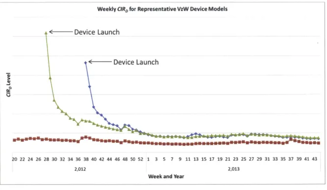
Examination of C/RD data over time for a number of Verizon devices reveals a consistent pattern of calling behavior for all devices. In the following figure, the C/RD data for several representative devices is plotted on a weekly basis over the course of 72 weeks between the spring of 2012 and the fall of 2013. This data reveals that for any device, the customer calling rate is highest at the time of market introduction for the device. Over time, the calling rate decays to a steady state level and remains fairly consistent over time. The steady-state level of C/RD varies by device model, but for all observed data the device calling behavior seems to follow this pattern.
Weekly CR0for Representative VzW Device Models
Device Launch
: Device Launch
20 22 24 26 28 30 32 34 36 38 40 42 44 46 48 50 52 1 3 5 7 9 11 13 15 17 19 21 23 25 27 29 31 33 35 37 39 41 43
2,012 2,013
Week and Year
Figure 6: Weekly CIRD for Representative VzW Devices
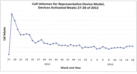
This pattern can be attributed to the logical behavior one would expect from any customer purchasing a new device. Upon activation of a new cell phone, it is rational to believe that a customer would have a high probability of calling into customer service. The customer is not yet familiar with the device, and any technical problems or questions regarding service plans are likely to come up when the device has just been activated. This concept is apparent from Figure 7 below, which shows weekly customer call volume for a representative device,
limited to customers who activated the device within a specific two-week time period.
The plot shows a burst of calls during the initial few weeks. Then as customers become more comfortable with the new phone and service issues are resolved, the call volume decays to a consistent level.
This behavior explains the decay pattern observed in the C/RD level over time in Figure 6. Initially, when a device is launched into the market, all of the device users are essentially new
Call Volumes for Representative Device Model, Devices Activated Weeks 27-28 of 2012
E
27 29 31 33 35 37 39 41 43 45 47 49 51 53 2 4 6 8 10 12 14 16
2012 2013
Week and Year
Figure 7: Call Volume for Devices Activated in Two-Week Time Frame
customers, for whom the device was just activated. In Figure 8 below, weekly active base over time for a representative device is presented, beginning with device launch. As more devices are sold into the marketplace, the proportion of experienced device users to new device users
Active Base for Representative VzW Device Model, Beginning with Device Launch
As Active Base increases, the proportion of experienced users to "new" device users increases, and thus CIRD decreases.
27 29 31 33 35 37 39 41 43 45 47 49 51 53 2 4 6 8 10 12 14 16 18 20 22 24 26 28 30 32 34 36 38 40 4244
2,012 2,013
Week and Year
Figure 8: Active Base for Representative VzW Device
increases. Given that the propensity of experienced users to call into customer service is low, the overall C/RD level decreases with time as the proportion of experienced device users increases.
At a given moment in time, the active base for any device model can be divided up into those devices which were recently activated and those which have been active for some time. The differing probability of placing a call into customer service for these groups forms the basis of the call forecasting model, to be discussed in a subsequent section.
2.2.2 Transient Factor
In addition to the device activation factor, observed CIRD levels over time tend to exhibit short-term fluctuations not related to device activation. These fluctuations are driven by transient market events which either stimulate or depress call center service demand for a brief period of time. In the plot below, the CIRD levels for a subset of Verizon Wireless devices are shown to demonstrate this transient behavior.
Weekly CIR, for Representative VzW Device Models, Transient Events Highlighted
Transient Events (Software Updates)
20 22 24 26 28 30 32 34 36 38 40 42 44 46 48 50 52 1 3 5 7 9 11 13 15 17 19 21 23 25 27 29 31 33 35 37 39 41 43
YearO Year 1
Week and Year
Figure 9: Transient Events, Software Updates
In the case of the above plot, the transient behavior is driven by device software updates. For most modern devices, both basic and smartphone devices, manufacturers have the ability to deliver software updates to add new features or correct problems with devices
currently in use. Software updates affect the operation of devices, typically upgrading device functionality but also potentially creating new problems. For many devices, software updates yield a noticeable transient shift in C/RD level.
In addition to software updates, transient events which can affect calling behavior include national holidays, wireless network outages and severe weather events. In the figure below, the transient effect of holidays is visible. The plot displays a weekly aggregate CIR level for the top twenty devices on the Verizon network (as of August 2013). In the weeks containing a major national holiday, the CIR level dips momentarily due to reduced demand for customer service. In addition, the week following a holiday tends to exhibit a slight increase in CIR level, due to customers delaying their service requests till after the holiday.
Weekly Aggregate CIR for Top 20 VzW Devices
National Holidays
20 22 24 26 28 30 32 34 36 38 40 42 44 46 48 50 52 1 3 5 7 9 1113 15 17 19 2123 25 27 29 3133 35 37 39 4143
Year 0 Year 1
Week and Year
Figure 10: Transient Events, National Holidays
For any forecasting model to be accurate, the effect of transient events must be taken into account. In the case of holidays and software updates, prior calling behavior can be used as a model for prediction. Since the schedules for both holidays and software updates are generally known in advance, past impacts can be used to predict future impacts. However,
both network outages and severe weather events are not predictable. Without advance knowledge of when such events may take place, it is difficult to account for them in any forecast.
For the forecast model implemented for this project, only predictable transient events (holidays and software updates) are taken into account.
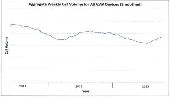
2.2.3 Call Volume Seasonality Factor
Incoming call volume to the call center system exhibits a noticeable seasonality, with the call volume peaking in the latter half of each calendar year and then decreasing into the first half of the following year. The figure below shows the seasonality pattern in aggregate call volume over the course of three years.
Aggregate Weekly Call Volume for All VzW Devices (Smoothed)
E
2011
I2012
I2013
Year
Figure 11: Seasonality in Aggregate Call Volume
This behavior is to be expected given the routine seasonal device activation pattern for Verizon Wireless and the wireless industry in general. Verizon tends to release the majority of
its flagship devices into the marketplace in the latter half of the calendar year to coincide with the increase in consumer spending into the holiday season. The figure below plots the sum of
weekly activations of flagship device models on the Verizon network in a representative year. (Flagship devices are those which are heavily marketed and attract the most customers. Such devices constitute a significant proportion of total active device count.)
Weekly Net Flagship VzW Device Model Activations
0
1 3 5 7 9 11 13 15 17 19 21 23 25 27 29 31 33 35 37
Year1
Week and Year
Figure 12: Flagship Device Activation Seasonality
Given that new device users have a higher propensity to call for customer service, the increase in new activations is accompanied by an increase in call volume. Thus, the seasonal behavior of gross call volume should primarily be explained by the device activation age factor, as previously described in section 2.2.1. However, when examining the CIRD level for several device models, there appears to be a slight seasonal increase in call volumes for some individual device models as well. (See Figure Below)
This seasonality contradicts the device activation age factor, given that the long term CIRD level does not simply converge to a static level, but rather seems to be influenced by the seasonality of gross device activations on the Verizon Wireless network. The devices which exhibit this behavior tend to be relatively older models which have been on the market for at least a full year. Most users of such devices have been using their devices for a long time, and
Weekly CIRD for Representative VzW Device Models, Seasonality Effect Highlighted
1 3 5 7 9 11 13 15 17 19 21 23 25 27 29 31 33 35 37
2,013
Week and Year
Figure 13: Seasonality in Device CIRD
perhaps may be considering upgrading to a newer model. Furthermore, given that the bulk of device activations take place in the latter half of the calendar year, many customers are coming to the end of their contracts within this time period and are able to upgrade at reduced prices. Given that the long-term C/RD levels tend to move with gross device activation levels, it is assumed that these users are calling into customer service to inquire about upgrading to the latest model devices. Such behavior would explain the observed slight seasonal shifts. This idea of seasonality influencing long term C/RD is the final component of the forecasting model developed for this project.
3 Forecast Model Proposal and Calibration
The following chapter describes the model formulation based upon previously described patterns discovered through data analysis. All data for call volume analysis was available on a per week basis, so the forecasting model was designed to forecast weekly call volume per device.
The model structure is presented in steps, with each step expanding the model to account for each of the three factors outlined in the previous chapter. After the model structure has been presented, the model calibration and fitting process is described.
3.1.1 Proposed Model Structure
The basic model formulation is inspired by mobile device return forecasting techniques developed for Verizon Wireless [1]. In prior research, the return rate for wireless devices was shown to be driven primarily by date of purchase. The warranty policy for Verizon cell phones covers the cost of replacement for a fixed period (generally one year from purchase). Thus, the device return rate was found to be relatively constant during the warranty coverage period, after which it would immediately fall to a minimal level. For this research project, the equivalent notion of customer service demand being driven by device age is applied in the forecasting model.
Given the device activation age factor described in section 2.2.1, the following initial model is proposed to describe user calling behavior. (See Figure Below) At the time of device activation, the propensity to call for customer service is greatest. After some time it decreases to a mid-level, and ultimately it settles to a steady-state level. These three temporal periods are represented by windows A, B and C in the below diagram.
Figure 14: Calling Behavior Model for New Activations
Given this model, when assessing user calling behavior for a given week, active devices can be split into three groups - new activations (activated within window A), recent activations (window B) and mature activations (window C). Thus, over the lifecycle of a device model D, for a given week n the incoming call volume CD(n) for the device is initially calculated as follows.
CD (n)= PA,DSA,D (n) + PB,DSB,D(n) + PC,D SC,D (n)
Equation 1: Initial Model
In this expression, PA,D, PB,Dand PCD are the number of calls received per device per week
for device model D for users in temporal groups A, B and C, respectively. The terms SAD(n), SB,D(n) and SCD(n) denote the number of active devices in temporal groups A, B and C, respectively. Thus, for each device model, the initial calculation of incoming calls for a week is accomplished by dividing up users according to device activation date and applying the above linear expression.
Note that in the context of this study, the only available statistic regarding device activation is the weekly active base count per device. Thus, the number of device activations which takes place in a week is assumed to be the increase in active base over that week. In
CORD
PA,D
PB,D
PC,D
User Calling Behavior Model
Time (Beginning with
Phone Activation)
reality this is not the case, as device de-activations will also take place, as in the following expression.
Active Base Current Week = Active Base Prior Week
+ Activations in Prior Week
- Deactivations in Prior Week
Due to the nature of the available data, for simplicity in this study the de-activation count is effectively ignored. Implications of this choice will be addressed in the discussion chapter. For parameters SAD(n) and SB,D(n), the values computed for analysis will be equivalent to the active base growth within windows A and B, respectively. In the case where a device active base is in decline, as for an older device model, the values of SA,D(n) and SBD(n) will be set to zero.
At this point the proposed model must be expanded to account for transient events. In the context of this project, both major holidays and device software updates are included as transient events. These events are assumed to affect all users of a device model, irrespective of device activation age. Thus, to include transients, Equation 1 above is expanded as follows.
CD(n)= PA,DSA,D(n)+ PB,DSB,D(n)+ PC,DSC,D(n)
+ TD (n)STOtal,D(n)
Equation 2: Incorporating Transients
In this expression, TD(n) is the transient function, which reflects the total transient impact in terms of number of calls per device for week n for device model D. The term STotalD(n) denotes the total active base for device model D in week n. (This term is equal to the sum of SA,D(n), SBD(n) and SC,D(n)) The transient function is to be constructed to account for both major
The final factor to be taken into account for the forecast model is the seasonality effect. The hypothesis drawn from data observations was that this effect was the result of users of older generation devices calling into customer service to inquire about the latest devices. The observed C/RD levels tend to increase with the seasonal increase in gross activations for new devices. Thus, the forecast model is further extended to account for this seasonal shift as follows.
CD(n)= PA,DSA,D(n)+ PB,DSB,D(n)+ PC,DSC,D(n)
+D (f)STotal,D(n)
+ HDG (n)STotal,D(n)
Equation 3: Complete Model
In this expression, G(n) denotes the total number of device activations of all models for week n. HD denotes the impact of seasonal device activations on call volume for users of device D. The product term HDG(n) reflects the increase in call volume in terms of calls per device for week n for device model D. The value of HD is distinct for each device and is expected to be greater for older device models, whose users may be looking to upgrade.
The completed model above was fit to input calling data for all devices using linear regression. The fitting process is detailed in the following section.
3.1.2 Model Fitting and Calibration
The first step required for model fitting is selecting appropriate data window lengths. The goal of the model is to construct a four month call volume forecast. Thus, calling data for all devices was divided into training and testing data, whereby a set number of weeks of calling data was used to fit model parameters, while the subsequent 16 weeks of data was used to
evaluate the model prediction accuracy. The number of weeks of calling data to use for model fitting was selected in order to yield an optimal forecast.
Given the pace of change in the mobile device marketplace, consumer behavior is likely to shift with time, and thus the model should try to capture recent information. However, the model must also capture enough information to ensure that the model fit is robust in the presence of data variability.
In addition to length of the fitting data window, the model as given in Equation 1 requires the choice of appropriate lengths for temporal windows A and B, as shown in figure 14. Window C encompasses all mature devices (those activated prior to windows A and B).
Defining window lengths a and b for windows A and B respectively, the active base counts referenced in Equation 1 are defined below.
SA,D(n) = Devices activated between week (n - a) and week n
SB,D(n) = Devices activated between week (n - a - b) and week (n - a)
Sc,D(n) = Devices activated before week (n - a - b)
Along with fitting data window length, appropriate values for a and b had to be selected such that the model would have optimal predictive value. To accomplish this, an experiment was conducted to test a number of parameter combinations. Input data window length (the
number of weeks of data used to fit the regression model) was varied between 20 and 40 weeks while the parameters a and b were varied between 0 and 3 weeks. For the purpose of this experiment, only the initial model given in Equation 1 was considered. Linear regression was applied to training data to determine the coefficient values PA,D, PB,D, PC,D for each device (using independent variables SAD(n), SB,D(f) and SC,D(n) and dependent variable CD(n)). These model coefficients were then applied to the subsequent 16 weeks of testing data to determine
the average percent error of the predictive model. This was repeated for all parameter combinations. (See Figure Below)
The results show that using a window length of 32 weeks, along with parameter settings a=1 and b=O, yields the optimal forecast results. (Setting the value of b to zero basically
Data Window = 26 Weeks Data Window
=
32 Weeks Data Window = 38 Weeksa
a
a1
b
b
b
Figure 15: Forecast Average Prediction % Error with Varying Parameters
removes the B window from the forecast equation entirely, and Equation 1 is reduced to having only two terms rather than three.) This is an interesting result - It shows that having a simpler forecast model that divides devices into only two groups based on activation time, rather than three, actually yields better predictive accuracy. This implies that the original three-group model was actually over-fitting to the data.
Having established the window parameters, the model is now expanded to account for transient events. To establish the time and impact of software updates, first a comprehensive list of updates was compiled for all devices. Then for each device, the CIRD level over time was examined to determine transient impact. This was done in a simple, ad hoc manner. In some cases, the impact of software updates was significant and easily noticeable (See Figure Below), but in other cases impact was indistinguishable from normal variability.
1 2 3 0 0.07638 0.09067 0.09154 1 0.09209 0.09370 0.09491 2 0.09622 0.09527 0.09744 3 0.09665 0.09890 0.09856 1 2 3 0 0.06766 0.08239 0.09150 1 0.08221 0.09265 0.09667 2 0.09344 0.09815 0.10351 3 0.09868 0.10605 0.10967] 1 2 3 0 0.06972 0.07993 0.08712 1 0.08015 0.08778 0.09198 2 0.08756 0.09129 0.09535 3 0.09147 0.09512 0.09872
Weekly CIRD for Representative VzW Device Model, Transient Event Highlighted
Software update impact on OIRD. __ Nominal level (without transient
event) shown as dottedline.
1 2 3 4 5 6 7 8 9 10111213141516171819202122 232425261
Year 1 Week and Year
Figure 16: Accounting for Transient Events
For those circumstances with noticeable transient impact, the nominal level of CIRD was inferred by looking at levels before and after the transient and interpolating the points between. This nominal level is assumed to be the level of CIRD which would have occurred if the software update had not taken place. The transient impact for a given software update,
measured in calls per device for week n, was calculated to be the difference between CIRD and the nominal level.
TD,Update(n) = CIRD(n) - NominalD(n) [For the given software update]
This method is analogous to how the impact of promotions is often calculated for sales forecasting. The impact of distinct promotions can be combined by superposition to find the full impact for sales over time. Such methods have also been used to assess the impact of promotions on call center demand [2].
For those software updates without any noticeable impact, it was assumed that this was a minor software change which did not yield any customer issues. Such updates were
effectively considered as non-events and removed from the database. Transient impact for all software updates for all devices was determined in this manner.
Prominent national holidays were assumed to affect all Verizon customers. To find these impacts, rather than analyze C/RD for all devices, the aggregate weekly CIR level for the top twenty devices (See Figure 10) was used. For the major holidays which exhibit a noticeable transient shift, the impact was measured in the same manner used for software updates. Note than in the case of holidays, transient shifts only occur for a single week, rather than several weeks as in the case of software updates. This is because software updates tend to have staggered distribution such that it takes several weeks for the update to be applied to all customers.
The final transient impact for device D for all weeks n is computed as the sum of impacts for all holidays and software updates.
TD(n) = THolidays(f)+ TD,Updates(f)
This transient function can be incorporated into the forecasting model shown in Equation 2 to improve model performance. In order to use the transient data, the linear regression process must be modified. Prior to the model fitting, the training data must be adjusted to remove the impact of the transient events. Essentially, this requires subtracting call volume attributed to transient events from the full call volume CD(n).
CD,Adjusted(n) = CD(n) - TD(f)STotal,D(f) [For Training Data]
After this correction, the linear regression is applied as before to the adjusted call volume data to determine the coefficients PA,D, PB,D, PC,D for each device. These can then be applied in linear combination to the 16 weeks of testing data to determine an initial call
volume. Finally, the 16 week call volume estimate is completed by adding the transient impact for those weeks back into the call volume.
CD(n) = CD,Adjusted(fn) + TD(n)STotal,D(n) [For Testing Data]
Accounting for transient events has the additional benefit of improving the potential accuracy of the regression coefficients, given that the adjusted data used in the linear regression is free of transient artifacts.
The final piece needed to complete device model fitting is the seasonality factor as given in Equation 3. The observed behavior revealed that there was an impact in C/RD related to the sales cycle for devices. In the case of customers who have been using their phones for some time, the release and sale of new devices appears to boost call volume.
Given the timeframe of the available data, a subset of device models was selected to build function G(n) in Equation 3.
G(n) = Sl,Dl(n) + Sl,D2(n) + S1,D3(n) +
In the above expression, S1,D1(n) is the number of activations of device model D1 which
have taken place within the 1 week prior to week n. Device models D1, D2, D3 and so on are selected to be the current flagship devices within the timeframe of the forecast fitting data. These are devices which will spur the most interest amongst current customers. G(n) is calculated as the sum in the expression above and is incorporated into the forecasting model as given in Equation 3. This element completes the model - The plot below displays an example of the application of the complete model to sample data.
Forecasting Example for Representative VzW Device
E
Training Data Testing Data
38 40 42 44 46 48 50 52 1 3 5 7 9 11 13 15 17 19 21 23 25 27 29 31
2012 2013
Week and Year
-Calls Estimate -Calls Answered
Figure 17: Example of Complete Forecast for Sample VzW Device
Note that the procedure for fitting and forecasting is the same as before. The training data must be corrected in advance to remove transient impacts, but now the regression is
applied to find an additional coefficient: PAD, PCD and HD (Note that PBD is no longer required, as the B window has been removed from the model). The parameter HD represents the impact of seasonal sales on call volume for device D. Using the window parameters already selected, the completed model yields an average percent error of 5.2% across all device models, an
improvement from the previous value of 6.7% (See Figure 15).
3.2 Potential Model Performance
Applying the completed model, the aggregate forecast performance can now be analyzed. In previous sections, the forecast model structure has been developed to
independently address device models. Now, the forecast output for all of the top 20 devices is summed over the 16 week span of testing data. This yields the results in the figure below.
Aggregate Call Forecast, Top 20 VzW Device Models
E .2
:9Training Data Testing Data
'5---1--- ---
---2 1 3 5 7 9 11 13 15 17 19 21 23 25 27 29 31 2013
Week and Year
-Calls Estimate -Calls Answered 38 40 42 44 46 48 50 1 2013 Week# % Error 16 0.005468805 17 0.02527215 18 0.014131713 19 0.00381784 20 0.006658774 21 0.045793972 22 0.059239403 23 0.007118692 24 0.026349561 25 0.074280454 26 0.018521097 27 0.092030636 28 0.075233318 29 0.047220075 30 0.066102036 31 0.047144584 Average 0.038398944
Figure 18: Aggregate Call Volume Forecast Potential Performance
The average percent error for the weekly forecast is 3.8%, and the maximum absolute error is 9.2%. The logical expectation for this aggregate forecast would be that the average percent error for the aggregate would be lower than that of the individual device models, assuming that the forecast error for all device models is mutually independent [3].
The results here do show a reduction in error, but this improvement is limited primarily because of the distribution of call volume amongst devices. While this analysis incorporates all of the top 20 Verizon Wireless device models, the actual call volume tends to be dominated by only the top few. Furthermore, there tends to be correlation in call volume in across devices in the case of software updates. For many device manufacturers, software updates for multiple smart phone models are released together. Thus, the transient impact of a software update can affect several device models at once. Any error in accounting for the update is magnified across more than one device.
The pareto chart below shows the distribution of call volume for the top 20 devices. The bulk of call volume is generated by the top few device models. Given this distribution, the error-cancelling effects that one would expect in the aggregate forecast are reduced.
Pareto Chart of Active Base Count for Top 20 VzW Device Models
W Top 3 VzW Models represent more than
30% of Tot aActive Devices
FA
M
Figure 19: Pareto Chart of Top 20 VzW Device Models
This performance analysis shows potential for the aggregate forecasting technique, but the last step in analysis is to assess performance in the case of true forecast device activations. Up to this point, all device calling and activation data has been drawn from the available dataset of prior values. Specifically, device activation data used to compute the independent variables SAD(n), SBD(n) and SCD(n) and G(n) (See Equation 3) for forecast testing data has been taken from the true dataset, ie., the actual data for activations. In an actual forecasting scenario, prior values would be used for training, but for the actual forecast the independent variables would themselves have to be estimated values.
This estimation is done using the device model sales forecast data, as described in the results chapter which follows.
4 Results
4.1 Device Sales Forecast Data
For the purpose of testing the live performance of the forecasting model, after fitting the model coefficients using prior data, the independent variables SAD(n), SBD(n) and SC,D(n) and G(n) for the 16 week forecast period must be estimated. Active base count data for the future is of course not available, but in the previous chapter it was established that the Verizon Wireless marketing division generates a 16 week sales forecast for all active device models. This data is used as a proxy for the active base data upon which the model was constructed and evaluated.
The sales forecast figures cannot be utilized directly. As discussed in Section 3.1.1, the calculated values used for SA,D(n) and SBD(f) are equivalent to the net increase in device active base within windows A and B, respectively. The sales figures account for all projected device sales each week via retail channels. They do not account for potential device activations which may occur when people obtain devices through non-standard channels, such as eBay or Craigslist. Furthermore, they do not account for device de-activations as do the active base statistics used to compute SA,D(n) and SB,D(n). Despite these distinctions, the projected sales figures still represent a significant portion of net active base change and are used for prediction as follows.
The 16 week sales forecast data is used to project the device active base for the same 16 weeks. This is accomplished by first making a simple observation. The plot below shows the active base count for several device models. Unlike the weekly call volume, the active base
count varies smoothly, with minimal variability from week to week. Furthermore, changes in the growth trend are gradual, with the slope of the curve shifting slowly over time.
Weekly Active Base for Representative VzW Device Models
41
2022242628303234363840424446485052:1 3 5 7 9 1113151719212325272931333537394143
2,012 2,013
Week and Year
Figure 20: Weekly Active Base for VzW Device Models
To project the active base for the subsequent 16 weeks, first a weekly shift trend RD is established by applying a weighted moving average to the prior five weeks of available active base data for each device in the following manner. (In the equations that follow, the most recent available week is referenced as week 0, and previous weeks are referenced with negative indices.)
RD
(
(Active Base Change between week (-4) and week (-3)) +(D= )
* (Active Base Change between week (-3) and week (-2)) +(18)
()-
* (Active Base Change between week (-) and week (-)) +( 18)
- * (Active Base Change between week (-2) and week (-0))+
(18)
This trend value serves as the baseline expected weekly shift in active base for device D over the next 16 weeks. The value is biased such that the highest weight is applied to the most
recent weekly change. This manner of moving weighted average is a common basic technique used for univariate forecasting. While more sophisticated techniques were considered [4], this method was chosen for its simplicity.
The sales forecast data is now used to project deviations from this baseline trend. This is done by taking a similar weighted average of the first four weeks of sales forecast data, with the greatest weight applied to the first week. This average value LD is then subtracted from all sales forecast values to find the deviations VD(n).
VD(n) = (Week n sales forecast for Device D) - LD
This function essentially captures how the sales forecast is deviating from the beginning trend over the course of 16 weeks. The assumption here is that the ending trend RD of the active base count shift corresponds to the beginning trend LD of the sales forecast. This is based upon the observation that active base for all devices varies gradually. The values of function VD(n) capture how the sales forecast is effectively varying from the expected level, and thus these values can be incorporated into the active base projection to account for changes in the expected level of sales over the next 16 weeks.
The final projection FD(n) is calculated as follows. n
FD(n) = FD(O)+ Y(RD + VD(k))
k=1
FD(n) is the projected active base for week n for device D over the course of 16 weeks. (Note again that week 0 is the latest prior week, thus FD(O) is the initial active base prior to the 16 week projection.) This projection is used to calculate the model input parameters SAD(n),
4.2 Forecast Model Performance
Having established projected data parameters for all devices, model performance can now be evaluated. For the case of the projection, the true impact on transient events is estimated based upon past behavior. National holidays are assumed to have to the same impact in the future as was the case in the previous year. Software updates are assumed to have the same impact in the future as similar software updates in the past. Note that since new software updates are different each time, the impact will likely not be the same, but for the purposes of forecasting this is an appropriate assumption.
The full forecasting process is summarized in the following, with the model fitting and forecasting processes separated.
Model Construction Call Forecasting
1. Gather historical Call Volume 1. Gather Device-Specific Sales and Device Activation Data Forecast data
2. "Correct" Call Volume Data in 2. Apply linear regression advance to account for coefficients to Sales Forecast
Transient Events Data to obtain Initial Call
3. Apply Linear Regression to Volume Forecast
determine device-specific 3. Apply "Corrections" to Initial behavior coefficients Forecast to account for
upcoming Transient Events
Figure 21: Complete Forecasting Process Steps
Applying this process with the latest 32 week window of device data and the 16 week device sales forecast yields the following aggregate call volume forecast for the top 20 Verizon device models. In the below diagram, weeks 4 through 35 of Year 1 are used as training data, while the weeks labeled FO to F15 are forecast.