Auto-adaptive and faster algorithm to optimize the calculus of the current flows in radiating structures

HAL Id: hal-00125960

https://hal.archives-ouvertes.fr/hal-00125960

Submitted on 3 Feb 2020

HAL is a multi-disciplinary open access

archive for the deposit and dissemination of

sci-entific research documents, whether they are

pub-lished or not. The documents may come from

teaching and research institutions in France or

abroad, or from public or private research centers.

L’archive ouverte pluridisciplinaire HAL, est

destinée au dépôt et à la diffusion de documents

scientifiques de niveau recherche, publiés ou non,

émanant des établissements d’enseignement et de

recherche français ou étrangers, des laboratoires

publics ou privés.

Auto-adaptive and faster algorithm to optimize the

calculus of the current flows in radiating structures

Pierre Dubois, Claude Dedeban, Jean-Paul Zolesio, Jean-Pierre Damiano

To cite this version:

Pierre Dubois, Claude Dedeban, Jean-Paul Zolesio, Jean-Pierre Damiano. Auto-adaptive and faster

algorithm to optimize the calculus of the current flows in radiating structures. Journées Internationales

de Nice sur les Antennes (JINA 2004), Nov 2004, Nice, France. pp.406-407. �hal-00125960�

AUTO-ADAPTIVE AND FAST ALGORITHM TO OPTIMIZE THE

CALCULUS OF THE CURRENT FLOWS IN RADIATING

STRUCTURES

P. Dubois

, C. Dedeban

, J.-P. Zolésio

, J.-P. Damiano

1

France Telecom Division R&D, Fort de la Tête de Chien 06320 la Turbie, France pierre.dubois@francetelecom.com, claude.dedeban@francetelecom.com,

2

CNRS-INRIA, Projet OPALE, 2001 Route des Lucioles, 06560 Valbonne, France Jean-Paul.Zolesio@inria.fr

3

Laboratoire d’Electronique, Antennes et Télécommunications Université de Nice-Sophia Antipolis – CNRS 250 rue Albert Einstein, 06560 Valbonne, France

damiano@unice.fr

Abstract

Accurate electromagnetic modeling is often too time-consuming. Solving electromagnetic scattering and radiation problems with moment methods or finite-element methods over a large frequency band requires the computer code to be run for every frequency sample. This is too expensive. So we propose a fast auto-adaptive method to optimize the calculus of the current flows for various radiating structures.

Introduction

The cost of computational electromagnetic simulation by the moment method or the finite-element method is expensive because the computer model has to be run for every frequency sample. But in recent years various interpolation algorithms have been developed and published [1-3]. Our aim is to obtain the current flows at the antenna surface over the frequency band using only a limited number of frequency samples, adding specific information based on the knowledge of the derivatives of these current flows [4-6]. Thus we have developed an original adaptive algorithm for which we present various results and comments for some structures.

Modeling

We propose an original method taking into account the formal knowledge of the derivatives of the variational expressions of the current flows. The numerical solution is obtained by a surface finite-element method coupled with an adaptive interpolation algorithm [5-6]. This approach takes into account the true electromagnetic behavior. From the frequency derivability results associated with the Huyghens principle for C2

surfaces we obtain the two derivatives of the Rumsey reaction [4] by a computer algebra system (Maple), and we then compute the unknown current flows and their derivatives at the antenna surface for a very small number of frequency samples. The expressions of the derivatives of the current flow become more complex when the order of derivation increases, and although the kernel singularity is never stronger than the original, integration of the successive kernels needs specific developments.

To solve the Rumsey reaction numerically we use a finite-element computer code (SR3D by France Télécom R&D). This is based on an integral equation formulation with triangular finite-element discretization. Thus the SR3D software solves an equation of bilinear form where the current flow X is the unknown. Therefore the derivatives of flows of current (X’, X’’) are also solutions of a linear system of the form: A . X = B. Operator A remains the same, only the second member changes: B’ for X’ and B’’ for X’’. The operator consists of the successive derivatives of A and B and of lower-order derivatives of the current flow. Once the successive derivatives of the unknown current flows are computed at some sampling points over the frequency band, our special adaptive interpolation routine is applied to evaluate them.

Interpolation

Interpolating and approximating a function by polynomials or rational functions appears difficult if only a small number of sample points are known, without other information.

Many kinds of interpolation methods exist [1-3,7-14], for example the well known least-square method, the Taylor series, the Newton, Lagrange, Chebyshev and trigonometric polynomial interpolations, the piecewise polynomial functions, the Padé and the Chebyshev or Chebyshev-Padé approximations, the Thiele interpolation, the spline functions, and so on. Rational approximations are sometimes superior to polynomials because of their ability to model functions with poles. It is quite difficult to determine the degree of the two polynomials. The interpolation by rational functions seems more stable, however when the known points of the signal are widely spaced oscillations also appear. This approximation is sometimes used by Computer-Aided-Design software analyzing general planar structures (Model Based Parameter Estimation (MBPE) or Adaptive Frequency Sampling modules). It allows the number of computed points to be divided by two or more. Other methods can be used in signal processing (basis functions, wavelet functions, etc.).

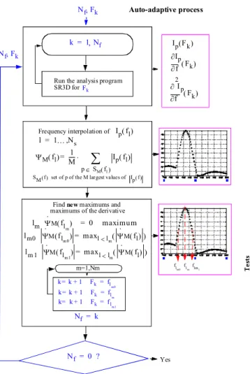
So we have developed an original and flexible adaptive fifth-order polynomial interpolation based on the knowledge of the derivatives of the current flows. This choice allows the number of frequency samples to be still further reduced (figure 1). In this flow chart we present our adaptive algorithm based on the detection of a "pathology" in the behavior of the function. It is based on the variations of the first and second derivative functions. An auto-adaptive algorithm to automatically identify new sampling points is exposed here. The new frequency points are related to the variations of a real function of the frequency, ΨM(f) defined from the M

highest values of the current flows (about 10% of the number of degrees of freedom). Thus this method clearly improves the localization of the concentrations of fields so as to detect the emergence of new resonances with variation of the frequency.

Our model gives better results than other methods such as simple polynomial interpolation, spline functions, or least square [5-6]. When there is only one peak in the original function the Thiele interpolation gives very good results. Comparisons are obtained between various interpolation results and our adaptive model with 7 points only for a 30% bandwidth. In the case of two or more peaks when the sample frequencies are equally spaced, Maple's formula for the Thiele approximation has singularities which cause it to fail. Some solutions exist but they do not always agree. We present a comparison between various interpolation results and our model with 7 points only for a 40% bandwidth (figure 2). We observe an excellent agreement between our original test function and the theoretical results.

Results

We consider a circular waveguide over the frequency band 4.6-6 GHz. This structure is meshed with 4,432 elements at 5 GHz. Using finite-element SR3D code and 70 frequency points we compute the reference variations of the VSWR (Voltage Standing Wave Ratio) over this band, given by a green curve. Figure 3 shows the comparison between this green reference curve calculated from the classical computed current flows and the interpolated variations of the VSWR obtained from the classical computed current flows (red curve). This is level 0 of the algorithm. The quadratic error is less than 5%. However we have "pathological" behavior around 4.9 GHz. So we run the adaptive version of our modified SR3D code to refine the data set around this frequency: this is level 1 of the algorithm. Figure 4 presents the refined VSWR obtained by adding one point to the uniform frequency set. We observe an excellent agreement between the reference and the new interpolated VSWR.

In the case of a line-slotted patch antenna the reference results of SR3D code are obtained with 55 frequency points. In figure 5 we present some examples of the efficiency of the adaptive algorithm. Part (a) presents the comparison of the average of the twenty highest values of the modulus of current flow versus frequency (4.5-6.0 GHz) for various numerical simulations. Part (b) concerns the quadratic average of the twenty highest values of the current flows. It is sufficient to give a excellent idea of the behavior of the real current flow. When we implement the first level of our adaptive algorithm we observe a very good alignment between the optimized curve (red curve) and the reference points (green circles). If the second level of the algorithm is applied, an excellent agreement is obtained (green curve).

Conclusion

We have presented an original and auto-adaptive optimization technique to calculate current flow at the antenna surface over a large frequency band with a very small number of frequency samples. Knowing the formal derivatives of the current flow, we are able to compute an accurate polynomial interpolation to obtain this current flow at the surface of the antenna. Comparing our results and those obtained by other techniques we observe an excellent agreement and a significant reduction in computing time (about 90%).

Run the analysis program SR3D for Frequency interpolation of Ψ_M( )f_l= _M---1 I_p( )f_l p∈SM( )fl

∑

SM f() set of p of the M largest values of Ip f() I_p( )f_l l = 1… N, _s l_m Ψ·Mf_l m ( ) = 0 maximum l_m0 Ψ·M(f_lm0)= max_{l lm<} (Ψ·M( )f_l ) l_{m 1} Ψ·M f_l m1 ( ) max_{l l} m < Ψ · M( )f_l ( ) = + + + f_l m0flmflm1 Fk

Find new maximums and maximums of the derivative

m=1,Nm k k 1= + Fk=fl_m0 k k 1= + Fk=flm k= k 1+ Fk=flm1 N_f = k k= 1 N, _f N_f,F_k N_f,F_k N_f =0 ? _Yes f ∂ ∂I_p F_k ( ) I_p( )F_k f 2 ∂ ∂ I_p F_k ( ) Auto-adaptive process

Figure 1 : Flow chart of the adaptive algorithm Figure 2 : Comparison between various interpolation _{results and our model with 7 points only for a 40%} bandwidth. Here a fifth-degree polynomial is used in

the least-square method.

Figure 3 : Variations of the VSWR - Level 0

Interpolation code (red curve).

Comparison with the reference (green curve).

Figure 4 : Variations of the VSWR - Level 1

Adaptive interpolation code (red curve). Comparison with the reference (green curve).

VSWR

2.0

1.6

4.6

5.0

5.4

5.8

From optimized and adaptive SR3D code

4.6

5.0

5.4

5.8

VSWR

2.0

1.6

1.2

(a)

(b)

Black curve : Numerical simulation including interpolation with 7 frequency

samples only.

Red curve : Simulation with first level

of refinement (2 additional points found by the adaptive algorithm)

Green curve : Second level of

refinement (3 new additional points found by the adaptive algorithm)

O : Values calculated by the classical SR3D code without any optimization

Figure 5 :

(a) Comparison of the average of the twenty highest values of the

current flows

(b) Comparison of the quadratic average of the 20 highest values of

the current flows

versus frequency (4.5 - 6.0 GHz) for various numerical simulations.

References

[1] P.L.Butzer and R.L.Stens, “Sampling theory for not-necessarily band-limited functions: A historical overview”, SIAM Review, vol.34, pp.40–53, 1992.

[2] E. Meijering, A chronology of interpolation : from ancient astronomy to modern signal and image processing, Proceedings of IEEE, vol.90, n°3, 319-342, 2002

[3] J.C. Rautio, Planar Electromagnetic Analysis, IEEE Microwave Magazine,vol.3, 35-41, 2003. [4] J.-P. Marmorat, J.-P. Zolésio, Rapport Contrat Armines-France Télécom, septembre 2000.

[5] J.P. Damiano, P. Dubois, C. Dedeban, J.P. Zolésio, P.Y. Garel, J.Y. Dauvignac, Original and accurate polynomial interpolation method to determine the surface currents with a minimum of known points in the case of diffraction and radiating problems, Proceedings of International Conference on Electromagnetics in Aerospace Applications (ICEAA), 2003, 8-12 sept., Turin, Italie, 491-494.

[6] P. Dubois, C. Dedeban, J.P. Zolésio, J.P. Damiano, Use of the frequency derivative of the harmonic regime for sensibility, European Congress on Computational Methods in Applied Sciences and Engineering, ECCOMAS 2004, Jyväskylä, Finland, 24-28 July 2004. [7] J. Yeo, R. Mittra, An algorithm for interpolating frequency variations of MoM matrices arising in the analysis of planar microstrip

structures, IEEE Trans. MTT, vol.51, n°3, 1018-1025, March 2003.

[8] X. Yang, E. Arvas, Use of frequency-derivative information in two-dimensional electromagnetic scattering problems, IEE Proceedings, Part. H, vol.138, n°4, 269-272, 1991.

[9] R. Lehmensiek, P. Meyer, Creating accurate multivariate rational interpolation models of microwave circuits by using efficient adaptive sampling to minimize the number of computational electromagnetic analyses, IEEE Transactions on Microwave Theory and Techniques, vol.49, n°8, 1419-1430, 2001.

[10] L. Xia, C.-F. Wang, L.-W. Li, P.-S. Kooi, M.-S. Leong, Fast characterization of microstrip antenna resonance in multilayered media using interpolation/extrapolation methods, Microwave and Optical Technology Letters, vol.28, n°5, 342-346, 2001.

[11] J.-L. Hu, C. H. Chan, T. K. Sarkar, Optimal simultaneous interpolation/extrapolation algorithm of electromagnetic responses in time and frequency domains, IEEE Trans. MTT, vol.49, n°10, 1725-1732, 2001.

[12] W. Koepf, Efficient Computation of Chebyshev Polynomials in Computer Algebra Systems: A Practical Guide (Ed. M. J. Wester). New York: Wiley, 79-99, 1999.

[13] C. Brezinski, Padé-Type Approximation and General Orthogonal Polynomials, Birkhäuser, Basel, 1980. [14] G. Micula, S. Micula, Handbook of Splines. Dordrecht, Netherlands: Kluwer, 1999.