HAL Id: halshs-03231786
https://halshs.archives-ouvertes.fr/halshs-03231786
Preprint submitted on 21 May 2021
HAL is a multi-disciplinary open access
archive for the deposit and dissemination of sci-entific research documents, whether they are pub-lished or not. The documents may come from teaching and research institutions in France or abroad, or from public or private research centers.
L’archive ouverte pluridisciplinaire HAL, est destinée au dépôt et à la diffusion de documents scientifiques de niveau recherche, publiés ou non, émanant des établissements d’enseignement et de recherche français ou étrangers, des laboratoires publics ou privés.
Urban economics in a historical perspective: Recovering
data with machine learning
Pierre-Philippe Combes, Laurent Gobillon, Yanos Zylberberg
To cite this version:
Pierre-Philippe Combes, Laurent Gobillon, Yanos Zylberberg. Urban economics in a historical per-spective: Recovering data with machine learning. 2021. �halshs-03231786�
WORKING PAPER N° 2021 – 33
Urban economics in a historical perspective:
Recovering data with machine learning
Pierre-Philippe Combes Laurent Gobillon Yanos Zylberberg
JEL Codes: R11, R12, R14, N90, C45, C81.
Urban economics in a historical perspective:
Recovering data with machine learning
aPierre-Philippe Combes
bLaurent Gobillon
cSciences Po - cnrs Paris School of Economics - cnrs
Yanos Zylberberg
dUniversity of Bristol May 2021
Abstract
A recent literature has used a historical perspective to better understand fundamental questions of urban economics. However, a wide range of histori-cal documents of exceptional quality remain underutilised: their use has been hampered by their original format or by the massive amount of information to be recovered. In this paper, we describe how and when the flexibility and pre-dictive power of machine learning can help researchers exploit the potential of these historical documents. We first discuss how important questions of urban economics rely on the analysis of historical data sources and the challenges as-sociated with transcription and harmonisation of such data. We then explain how machine learning approaches may address some of these challenges and we discuss possible applications.
Keywords: urban economics, history, machine learning
jel classification: R11, R12, R14, N90, C45, C81
aWe are grateful to Cl´ement Gorin for very helpful discussions, as well as to Gilles
Duran-ton and two anonymous reviewers for useful comments. The authors acknowledge the support of the ANR/ESRC/SSHRC, through the ORA grant ES/V013602/1 (MAPHIS: Mapping History). Laurent Gobillon acknowledges the support of the EUR grant ANR-17-EURE-0001.
b
Sciences Po - cnrs, Department of Economics, 28, Rue des Saints-P`eres, 75007 Paris, France. [email protected]. Also affiliated with the Centre for Economic Policy Research (cepr).
c
pse - cnrs, 48 Boulevard Jourdan, 75014 Paris, France. [email protected]. Also affiliated with the Centre for Economic Policy Research (cepr) and the Institute for the Study of Labor (iza).
dUniversity of Bristol. Also affiliated with the CESifo and the Alan Turing Institute.
1
Introduction
A recent, flourishing literature exploits historical data in order to understand the fundamental mechanisms underlying the spatial distribution of economic activity across countries, across regions or cities within countries, or across neighbourhoods within cities. Historical patterns of spatial development may indeed shed light on: the role of agricultural productivity on
ur-ban development (Matsuyama, 1992; Nunn and Qian, 2011); the long-term drivers of urban
structure within and between cities (Ahlfeldt et al., 2015; Siodla, 2015; Redding and Sturm,
2016;Heblich et al.,2021b;Hornbeck and Keniston,2017), and the specific role of
transporta-tion (Baum-Snow, 2007; Duranton and Turner, 2012; Brooks and Lutz, 2019; Heblich et al.,
2021a); the effect of transportation on the spatial distribution of economic activity (Atack,
2013; Donaldson and Hornbeck, 2016; Donaldson, 2018; Campante and Yanagizawa-Drott,
2018; Pascali, 2017; Trew, 2020) and the role of distance and communication in sustaining
economic exchanges (Bossuyt et al.,2001;Bakker et al.,2021;Juh´asz and Steinwender,2018;
Steinwender, 2018; Barjamovic et al., 2019); migration and how it shapes intergenerational
mobility (Olivetti and Paserman,2015; Abramitzky et al., 2012, 2021b;Ager et al., 2019).
These contributions often rely on large and scattered data sources which require digitisation and the creation of a consistent data structure. Digitisation includes the scanning of docu-ments and their transcription. The former, document imaging, is a costly process—usually undertaken by libraries and archives. The latter is a crucial step, yet often overlooked, and involves the recognition, encoding and labelling of features in scanned documents (e.g., table structure, images, manuscript characters). One example is the digitisation of transport
infras-tructure or borders on scanned historical maps (e.g.,Baum-Snow,2007;Duranton and Turner,
2012; Michalopoulos and Papaioannou,2013;Donaldson, 2018). The output of such a digiti-sation process may lack the structure and properties of a consistent dataset with well-defined variables (columns) and identifiers (rows). Harmonisation of variables and entry linkages are frequently needed. A recent example is the systematic linking between Census records,
con-scription lists or immigrant cards (e.g., Olivetti and Paserman,2015;Abramitzky et al.,2012,
2014;Ager et al.,2019). These different tasks share two common features: (i) they require the recognition of patterns across inconsistent sources; (ii) the amount of data limits the scope of labour-intensive solutions. Predicting patterns across numerous, noisy observations is a chal-lenge that is common to many research fields, which led to the widespread adoption of machine
learning techniques (seeMullainathan and Spiess,2017;Wager and Athey,2018;Athey,2019,
for applications in economics). This adoption—outside of census linking—remains however limited in urban economics and economic history, in spite of its obvious appeal.
In this paper, we discuss the possible use of machine learning for the creation of datasets from historical sources for urban economics. The analysis proceeds in three steps: (i) we
describe important research questions relying on the treatment of historical data; (ii) we present challenges associated with the transcription and harmonisation of historical data; (iii) we discuss machine learning approaches to addressing these issues, illustrating them with a few applications.
2
Research questions in urban economics relying on
his-torical data
The urban economics literature has made use of historical data, sometimes dating back to the archaeological period, in order to study spatial relationships and economic theories related to agriculture, urbanisation, growth, trade, mobility, and segregation among others. Information sources are often scattered across documents of various, unusual formats; they are so far mostly transcribed and coded by hand with non-automated processes. This collection process has hampered the use of data sources requiring significant data processing: for example, the manual extraction of information from scanned Census records is a long and strenuous task even for a team of research assistants, and the treatment of noisy raw information may not be consistent between individuals or over time. In this section, we show that important economic questions rely on access to historical sources that require significant processing. In that perspective, using more systematic predictive methods could prove attractive.
Note that our references to the literature are not meant to be exhaustive but rather illus-trative of the potential of historical documents for key research questions in urban economics.
2.1
Agricultural productivity and urbanisation
An important question of urban economics is whether and how historical agriculture expan-sion influenced urban development and productivity in the long run. There are interesting theoretical mechanisms relating agricultural productivity to economic growth across countries, and the same mechanisms can be transposed to within-country settings in order to study local
growth and the development of cities. Matsuyama (1992) shows that the effect of agriculture
productivity on growth depends on the ability to trade. If trade costs are prohibitive, a posi-tive relationship between agriculture productivity and growth can be predicted from a shift of labour from agriculture to manufacturing, where agglomeration economies take place. Indeed, fewer workers are needed for subsistence and extra ones can be allocated to manufacturing. In stark contrast and because of a comparative advantage mechanism, the reverse holds true when it is cheap to trade goods across space. Locations characterised by a higher agriculture productivity specialise in agriculture and do not develop much of their manufacturing. The
relationship between the development of agriculture and later economic growth is thus unclear and depends on transport costs and the resulting patterns of trade.
An empirical approach would consist in estimating the relationship between current
out-comes and past agricultural productivity. Nunn and Qian (2011) exploit the introduction of
potato cultivation in the Old World to assess the effect of agricultural productivity on popula-tion density: potato cultivapopula-tion is shown to account for one-quarter of urban growth between 1700 and 1900. Several empirical studies documenting the long-run impact of agriculture rely
on data that could be transcribed manually. For instance, Olsson and Paik (2020) use (i)
georeferenced archaeological sites located in the Western core of agricultural diffusion (Eu-rope, Middle East, North Africa, and Southwestern Asia) and (ii) digitised maps of regional Neolithic vegetation to show that regions transitioning to Neolithic agriculture earlier are now poorer than late adopters.
Historical information can be complemented by FAO’s GAEZ data about the local soil suitability to different types of agricultural production and technology, which allows to
char-acterise the local potential for agriculture. For instance, Fiszbein (2021) shows the impact
of agricultural diversity on long-run development across U.S. counties, Mayshar et al. (2019)
study the role of agriculture in the formation of the state, and Galor and ¨Ozak (2016) assess
the extent to which historical returns to agricultural investment affect time preferences today. This literature could gain from a better understanding of agricultural organisation in the past and its relation to the transport network and urbanisation. Transport infrastructure
affects agricultural returns through improved market access. For instance, Donaldson and
Hornbeck(2016) show that agricultural land values increased substantially when the railroad network expanded over the 1870–1890 period in the US. However, documenting the joint evolution of land use and urbanisation in the long run or the dynamics of agricultural produc-tivity and the determinants of structural transformation over time requires the digitisation of additional data. Agricultural censuses are needed to reconstruct the spatial distribution of agricultural productivity across regions over time. Land use and transportation infrastructure can be obtained from the transcription of a large set of map collections, for which the
infor-mation is not yet encoded.1 Such transcription can rely on machine learning techniques, such
as random forest or neural network approaches described in Sections 4.2 and 4.3 respectively.
2.2
Urban growth, city structure and transport
One important determinant of local development is the transportation network and its gradual expansion within and across cities over the past centuries. Transport infrastructure shapes the
1Two authors of this paper, Pierre-Philippe Combes and Laurent Gobillon, have a series of projects along
distribution of economic activity through changes in market access and transportation costs, sometimes persistently so. A number of applications assess the impact of past trade routes on
contemporary economic outcomes. Bleakley and Lin (2012) study the effect of past portage
sites along fall lines in the US on current population density using maps, historical reports and atlases as well as recent census and satellite night-time lights data. The effect of these original
locational advantages persists to this day, long after these advantages became obsolete.
Duran-ton and Turner (2012) show how the interstate highways network around a city boosts urban development. In order to isolate exogenous variations in the density of the interstate highways network, they rely on historical maps of transportation infrastructure, the interstate highway system and its original plans—which they complement by the digitisation of the 1898 railroad network and exploration routes from the sixteenth to the nineteenth century. Information on the transport network in England and Wales in the eighteenth and nineteenth centuries is
used by Trew(2020) in a quantitative model where transportation evolves endogenously with
trade, agriculture and manufacturing outputs. Better transportation infrastructure is shown to hamper structural transformation by dispersing economic activity across space, thereby reducing agglomeration spillovers.
Urban economics also studies the internal structure of cities, their hinterlands, and their
evolution over time. Baum-Snow (2007) uses the interstate highway original plans to study
the effect of transportation on the city structure. The interstate highway system, and the associated density of roads connecting city centres to their suburbs, are shown to be respon-sible for the suburbanisation of US cities over the second part of the twentieth century. A similar flight to the suburbs occurred in London between the late nineteenth century and early
twentieth century, with the development of public transportation (Heblich et al.,2021a). The
resulting separation of workplace and residence allowed the economic activity to concentrate around the City of London, thereby generating important agglomeration spillovers.
The previous research questions would benefit from more systematic approaches to the recovery of transport infrastructure from historical maps (e.g., the neural networks described in Section 4.3), especially so when transportation networks are dense, or mixed (with railroads, roads of different types), and manual data collection becomes tedious.
Analysing the drivers of city structure leads to the question of its persistence over time, as often documented through the persistence of residential segregation related to
environmen-tal (dis)amenities.2 Lee and Lin (2018) show how natural amenities shape neighbourhood
composition within U.S. metropolitan areas; Villarreal (2014) identifies drainage conditions
as a crucial factor in explaining urban development in New York; Heblich et al.(2021b) show
2The persistence of city structure is also shown through the long-run impact of an impermanent transport
infrastructure, i.e., street cars in Los Angeles (Brooks and Lutz, 2019), or past zoning/redlining policies (Shertzer et al.,2018;Aaronson et al., 2020).
how coal-burning factories of Victorian England generated a persistent East-West gradient in neighbourhood composition. The persistence of city organisation can be overturned by large shocks to urban structure. Recent contributions have shown the impact of urban renewal
us-ing bombus-ing in London (Redding and Sturm, 2016), the Great Fire in Boston (Hornbeck and
Keniston, 2017) or the San Francisco earthquake (Siodla,2015), as exogenous redevelopment factors.
Understanding the drivers of city structure requires collecting data on residents (e.g., Cen-sus records), firms (e.g., trade directories, the ancestor of yellow pages), transportation and other public amenities (e.g., city maps). Whilst these resources usually exist for large cities of developed economies and cover—at least—most of the twentieth century, their systematic ex-ploitation is challenging. For instance, most trade directories are manuscript and not yet even scanned; Census records include fragmented, noisy information (e.g., the address), or precise information that necessitates harmonisation (e.g., occupations or administrative units). The need for significant data processing has often limited studies to the analysis of one city at a
time, whether it be Berlin (Ahlfeldt et al., 2015), London, San Francisco or New York.
2.3
Communication, transport, and trade
Information from old ages has been used to study the patterns of trade and the role of transport and communication infrastructure. This requires quantifying trade flows and identifying the role of transport infrastructure in shaping these flows.
A literature studies ancient trade, relying on scarce data sources stored in unusual
for-mats. The recourse to automated methods may not add much to applications such asBakker
et al. (2021), who illustrate the relationship between connectedness and development using geographical information and a georeferenced list of archaeological sites (the Pleiades Project).
By contrast, machine learning may be of use in settings such as that ofBossuyt et al. (2001)
and Barjamovic et al. (2019) who use ancient administrative and commercial clay tablets to
identify political and economic interactions between cities. Bossuyt et al. (2001) isolate
refer-ences to other cities in records of transactions, contracts, and inventories for Mesopotamian cities in the third millennium BCE. They show that bilateral city citations are well explained by physical distance, testifying for a very early gravity pattern in political and economic
rela-tionships. Barjamovic et al.(2019) use commercial records produced in the nineteenth century
BCE by Assyrian merchants, and later transcribed in the “T¨ubinger Atlas des Vorderen
Ori-ents”, to evaluate a model of gravity using ancient trade routes. The original tablets include diplomatic letters, census and tax records, and inventories. The authors rely on textual anal-ysis to extract and isolate transactions, reconstitute trade routes and ultimately predict the whereabouts of cities whose location is still debated among historians. For this kind of studies,
one can imagine using machine learning to extract symbols from pictures of tablets and extract raw information with the support of archaeologists and automatic translation methods (e.g., using neural networks presented in Section 4.3). Image recognition methods coupled with machine learning may also help locate ancient settlements through the detection of buried
archaeological sites from aerial images (see Guyot et al., 2018, for instance).
Another literature shows how transport infrastructure shapes trade flows and income over the long-run, using historical transport networks either as an instrument or as the object of
the study itself. For instance, Duranton and Turner (2011) use historical maps of highways,
railroads and exploration routes to study the impact of road supply on road flows, showing in
particular that new transportation infrastructure does not decrease traffic congestion.
Don-aldson (2018) provides evidence on the extent to which Indian railroad network decreased trade costs, and increased trade and real income, when it was introduced over the 1870–1930 period.
The literature has also examined the relationship between communication and market in-tegration. This usually requires extensive information about transaction records and/or about
the transmission of information. Koudijs (2015) studies how private information transmitted
by boats sailing between London and Amsterdam at the end of the eighteenth century is in-corporated into prices of English securities. Information on arrivals of boats in Amsterdam and prices are collected from newspapers. Informed agents strategically trade securities such that prices in Amsterdam tend to co-move with those in London after the departure of boats.
Steinwender (2018) studies how information frictions distort transatlantic trade in the mid-nineteenth century, exploiting the introduction of the telegraph and its effect on prices and trade flows for cotton. Using data from newspapers, she finds a convergence of prices across the Atlantic ocean after the introduction of the transatlantic telegraph, coupled with larger
and more volatile trade flows. Juh´asz and Steinwender (2018) extract shipping information
from a daily, London-based publication, to investigate the drivers of trade in the nineteenth century cotton textile industry. Their study illustrates the potential of an automated ap-proach to the digitisation of historical newspapers: they use optical character recognition to convert the scanned images of publications into text files, which are then processed through a text matching procedure to extract the relevant information. The newly-processed data on trade records is used to show the role of communication in fostering economic exchanges across space: the introduction of the telegraph had a large impact on trade, especially so for
products that are the most easily codifiable.3
3Whilst these studies are interested in international communication, one can imagine conducting similar
exercises within countries in an urban economics perspective, relying on digitisation and machine learning approaches to extract economic transactions or shipping records from paper documents.
2.4
Migration and intergenerational mobility
A large literature at the fringe between urban economics, development economics and labour economics describes the movement of workers across space, analyses its determinants and its long-run impact on the sending and receiving ends.
Analysing the distribution of economic activity across space and over time requires under-standing the movement of the main economic factor, i.e., labour, which presents two main chal-lenges. First, researchers need to collect individual-level information from historical records (e.g., Censuses, conscription lists, immigration cards, passenger lists) which requires the scan-ning and transcription of handwritten or inconsistent notes. Second, constructing migration flows or isolating changes in the economic activity of workers implies linking entries from differ-ent data sources without consistdiffer-ent iddiffer-entifiers. In stark contrast with the literature presdiffer-ented in the previous section, the mobility literature has built upon earlier census linking efforts (Ferrie, 2005; Long and Ferrie, 2013) and incorporated systematic procedures to handle data
(often related to the exploitation of U.S. Census records and conscription lists, see
Feigen-baum, 2016;Abramitzky et al., 2021a, and sometimes using machine learning techniques, as described in Section 4.4.), thereby showing the research multiplier induced by cleaning and linking invaluable historical sources.
With mobility costs, there may exist different returns to labor across space. Abramitzky
et al. (2012) and Abramitzky et al. (2014) analyse the returns to international migration during the Age of Mass Migration in the United States (1850–1913), comparing labour returns at destination with returns at origin and with the performance of natives. These returns to
migration depend on cultural assimilation (Abramitzky et al.,2020a,b), and are passed on from
the first generation of immigrants to the subsequent generations (Abramitzky et al., 2021b).
These contributions have benefited from the systematic linking across historical records, e.g., across Census waves or between Censuses and immigration lists. The construction of migrant flows between regions, as well as between and within cities, allows a better understanding
of their impact on labour markets at destination (Boustan, 2007; Boustan et al., 2010), the
selection into migration and its impact on racial inequalities (Collins and Wanamaker, 2014,
2015), or the dynamics of income segregation patterns within cities (Lee,2020).4
While this recent literature sheds some light on the drivers of mobility and its impact on the distribution of economic activity and urbanisation in the United States, there remain large gains in assessing the general role of mobility and relocation rigidities in the rest of the world. This investigation would require to adapt/extend the systematic data processing that have
4A related literature, focusing on intergenerational mobility (Olivetti and Paserman, 2015; Feigenbaum,
2015;Ager et al.,2019) has also contributed to the development of systematic linkage procedures, identifying father-son pairs at prime working wage from the household structure recorded in one Census wave (the ‘fathers’ wave) and a link with a subsequent Census wave (the ‘sons’ wave).
been used in the U.S. to diverse economic environments.
3
Challenges with the treatment of historical data
The previous section has highlighted the possible research multiplier from the systematic exploitation of historical data. It has also indirectly emphasised two obstacles: (i) historical data are stored under unusual formats, especially those of interest for urban economists (e.g., handwritten records, newspaper articles, maps, old photos), and they require non-negligible transcription efforts once scanned; (ii) the data lack the inherent structure of usual data sources (e.g., proper identifiers) and thus require initial processing before they can be linked across sources.
3.1
Transcription of manuscript documents and tables
A large number of historical sources store information as manuscript or typeset text, e.g., micro-census records, transaction records, trade directories, immigration cards, ship registers, newspaper articles. The information may be subdivided and organised into bespoke tables, e.g., national or local statistics, prices of traded commodities. In this section, we briefly discuss the challenges associated with the systematic transcription of such data sources.
The textual transcription of scanned historical documents can be divided into two distinct tasks: (i) the reconstitution of the original text into computer-readable data; and (ii) textual
analysis (seeHirschberg and Manning,2015;Gentzkow et al.,2019, for a discussion of advances
in natural language processing and for a description of the use of text as data in economics). The first task involves the visual recognition of characters by a machine or by a human; the most obvious example is the digitisation of census records by the Mormon Church in the United States. Up until recently, only humans could deal with the visual recognition of irregular manuscript characters. Optical Character Recognition (OCR) based on deep learning
methods described in Section 4.3 are now an alternative.5 The most favourable scenario is one
in which the data is typeset into an organised table. Even then, and even if some methods now try to process entire documents at once, each scanned page needs in general to be broken down into columns and rows—which may involve the identification of anchor points (e.g., a line), the flattening/rotation of the image, the identification of lines through blurring or thresholding. Once a cell is isolated, its content can finally be extracted by machine learning.
5Note, however, that visual recognition algorithms require training sets, i.e., a partial transcription of the
document, on which the algorithm is calibrated. This ex-ante classification is often done by humans. However, new machine learning tools are currently developed to automatically generate training sets, or adapt existing training sets to new contexts, which is called ‘transfer learning’.
The second task, textual analysis, consists in extracting organised information from un-structured computer-readable text. A text is a meaningful sequence of words, each word carrying some information in its relationship with other, contiguous words. The purpose of textual analysis is to store this complex information into a limited set of well-defined variables, and the challenges associated with this task relates to the interlinked structure of language. An example extracted from a tablet from the Bronze Age and describing an economic transaction
illustrates these issues (seeBarjamovic et al., 2019):
In accordance with your message about the 300 kg of copper, we hired some Kaneshites here and they will bring it to you in a wagon... Pay in all 21 shekels of silver to the Kaneshite transporters. 3 bags of copper are under your seal...
Researchers interested in properly coding the previous transaction need to identify and relate goods (copper, silver), quantities (300 kg, 21 shekels, 3 bags), transportation (wagon) and par-ties (we, Kaneshites, you). The identification of separate notions or concepts may be difficult given the lack of a bespoke, segmented dictionary for each notion. For instance, horses can be a good or means of transportation. The combination of the separate notions is even harder to transcribe. In the previous example, the 300 kg of copper and the bags of copper are one and only object, mentioned before and after the payment for transportation. The extraction
procedure considered by Barjamovic et al. (2019) thus relies on a pre-identified dictionary of
cities to detect itineraries and ignores the more complex linkages between itineraries, transport mode, goods and quantities. The richness of the human language requires the use of
classi-fication or extraction algorithms that allow for a rich representation of texts (see Gentzkow
et al., 2019, for applications of machine learning to text analysis).
3.2
Transcription of features in historical maps
Accurate maps have been researched and drawn as a way to store and transmit information
about crucial, strategic data which may be of interest to the researcher in economics,6 e.g.:
physical geography; cities and communication networks; fire risk; land ownership; spatial poli-cies (designation of poor neighborhoods or slums); the spatial coverage of a disease outbreak. Preliminary steps in transcribing features of historical maps are (i) to scan the original material to obtain a computer-readable image (for instance, encoded as three variables, red, green and blue, for each pixel) and (ii) to georeference the output (i.e., to superimpose a coordinate refer-ence system such that each pixel can be localised on the earth surface). Even a geo-referrefer-enced image has distinctive features that complicate the extraction of information. In this section, we characterise these features using extracts of iconic map series which contributed to setting
6SeeNagaraj and Stern(2020) andNagaraj(2020) for a discussion of the incentives and constraints behind
cartographic standards worldwide: the Cassini Map from the 1750s, Etat-Major (i.e., Mili-tary) maps from the 1850s and Scan50 maps (aerial photographs) from the 1950s, covering France; and Ordnance Survey Maps covering England and Wales around 1880–1890s.
Maps are a repository of unorganised data: writings, symbols, lines/segments, and coloured surfaces are often grouped together on the same map tile and correspond to different pieces of information that has to be converted into separate variables. This implies that the nature of the data to be collected on the map tile requires to be determined by the extraction pro-cedure. Formally, one may want to isolate each feature on the map even when these features overlap. Several machine learning approaches can be implemented for that purpose. Support vector machines or decision trees can be used to distinguish surfaces of different nature (e.g., different land uses) and classify them into discrete categories. Neural networks make it possi-ble to recover and distinguish writings, symbols and lines (e.g., transport networks versus the delineation of complex buildings). Before getting into more detail about these procedures in Section 4, it is worth stressing specific issues related to the transcription of maps.
First, the display of different, conflicting information can make the attribution of the right category to each pixel quite challenging. For instance, symbols and writings might disrupt algorithms trying to recover the nature of the underlying surface. The recovery of some pieces of information may require to identify, or reversely ignore, other features. Reciprocally, the identification of symbols and names may be hard when superimposed on coloured surfaces. Figure 2(a) from the Cassini Maps shows the French port city of La Rochelle surrounded by writings and mills symbols on specific surfaces.
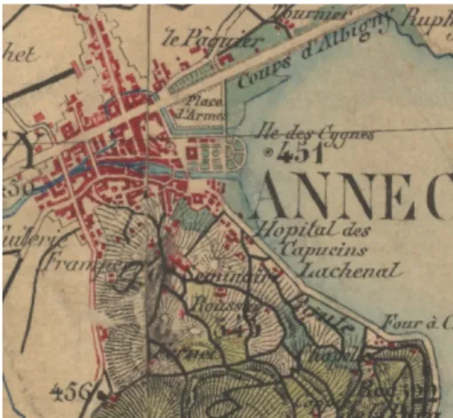
Maps may feature contour level lines to indicate topography; these lines could cut areas corresponding to uniform land use, as shown in Figure 2(b) (Etat-Major Map, south of An-necy, France). Lines indicating land use or contour level may interfere with administrative boundaries. These lines, representing different features, might be drawn in the same color and be hardly distinguishable from one another. Figure 2(c) (Etat-Major Map) displays one of those many instances of conflicting lines, around the French village of Cugn(e)aux.
Second, within data categories (e.g., cities, roads, plain areas), the researcher may want to recover specific details characterising a feature. One issue is that the representation of different feature types may be similar, and the representation of similar features may differ. This is often the case with simplified features, such as cities that may be represented as uniformly coloured surfaces without individual delineation of buildings or blocks. We illustrate this issue with the French city of Nevers for which only large built-up areas and the main roads are drawn—see Figure 2(d) (Cassini Map). Transport networks may be stylised and represented as a uniform plain line (without information on whether roads are narrow or large); alternatively, there may be different types of lines corresponding to different transport capacities. For medieval towns, fortifications may be represented in the same colour as built-up areas, and algorithms may
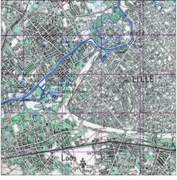
have hard time discarding them as such—as illustrated in Figure 2(e) (Etat-Major Map) with the fortifications of Strasbourg. Figure 2(f) (Scan50 Map, Lille) shows that many buildings are coloured in white, becoming hardly distinguishable from roads. Conversely, conventions to represent the same feature may differ: Whereas larger built-up areas may be represented with stripes, smaller ones may be uniformly filled.
Third, there exist a myriad of issues related to the quality of the original material which can be classified as: (i) the noise induced by the nature of data reporting (manuscript); (ii) the noise associated with storage and scanning; and (iii) the geographic nature of the stored infor-mation (e.g., the reference system used). These sources of noise interfere with data extraction, and a preliminary cleaning is often needed. For instance, characters may be drawn differently, with different fonts, and be reported with an angle. This is shown for the Ordnance Survey map covering Burnley, a factory town close to Manchester, in Figure 2(g). Colours or filling of objects may involve stripes or hatching and be mistaken for delineation lines or contour levels. This is the case for various series of the Ordnance Survey as shown on Figure 2(h) (Bristol). Different parts of a given map may have been drawn by different cartographers, at different time, or may be more or less damaged due to age; colours may thus not be consistent across map tiles as shown for the Etat-Major Map covering Paris (Figure 2(i)). The fragmentation of the geographic information across different map tiles may induce other inconsistencies, for instance, related to imperfect junctions between tiles (see Figure 2(j), Etat-Major map cov-ering the French town of Ruestenhart). Folds of the original map may appear as lines in the scanned images at the disposal of researchers. Finally, the territory covered by different map series may change over time as a result of boundary modifications due to wars and reparations; the harmonisation of boundaries may be a challenge.
3.3
Linkages across data sources and harmonisation
An often-overlooked component of data construction is the creation of a structure around well-identified variables and identifiers. This data structuring has been disciplined by the re-cent availability of, and need for, computer-based operations (e.g., the merge between datasets along a set of identifying variables); historical data sources often lack this inherent structure. For instance, one individual in a Census is not given any unique identifier and Census enu-merators are not particularly careful in reporting information (name, age, address) that would allow to recognise the individual in other data sources. In a similar vein, the name of a parish or district may change over time and there exist no look-up tables or keys linking adminis-trative units before and after repartitioning. Even more problematic, the repartitioning of administrative units through merges or splits are very frequent, because of political incentives (Bai and Jia, 2021), or less often because of changes in physical geography (Heldring et al.,
2019). Sometimes, it is possible to identify the timing and nature of changes from admin-istrative records, as the ‘Cassini project’ did with all mergers and splits for 40,000 French
municipalities since 1793.7
In the absence of identifiers (e.g., a social security number), researchers need to identify a set of variables which may help identify related observations across data sources. An immediate example is the use of names, age and birth location to link census records. Another example is the description of an address or a trade in directories. In both cases, the same information in different sources may differ due to reporting guidelines, or measurement error at the numerous, distinct stages of data collection and extraction. A matching procedure thus requires sufficient flexibility to allow for imperfect, ‘fuzzy’, matching. Given this description, linking records or observations requires to recognise noisy patterns across inconsistent data sources, an exercise similar in nature to pattern recognition within similarly noisy data. Machine learning has been developed to address this specific issue of pattern recognition and classification and its use is natural in this context, as we present in Section 4.4.
4
Machine learning methods and applications
In this section, we describe concrete applications of some machine learning approaches to urban economics.
4.1
An introduction to machine learning
Before we proceed, it is worth reminding the initial main difference between machine learning and econometrics. Consider a relationship, Y = f (X), between two variables, X and Y .
Economists are usually interested in obtaining an estimate bf (.) of function f (.), which usually
reflects an economic relationship. By contrast, machine learning has mostly been used to
produce an empirical prediction of the outcome, bY , knowing X.8
As a consequence, the econometrician estimates a single and best-suited model using the explanatory variables and assuming a functional form for f (.) that are relevant according to theory. This yields a unique prediction of the dependent variable Y for any combination of the explanatory variables. In machine learning, the researcher may estimate many distinct models, which differ from one another because they are based on different subsets of explana-tory variables and sometimes on different random sub-samples as in bootstrap econometric approaches. These distinct models yield different predictions of the dependent variable for the
7Seehttp://cassini.ehess.fr/for a description of the project in French.
8A recent, fast-growing literature however discusses the use of machine learning for identification of
treat-ment effects and inference (see, e.g., Wager and Athey, 2018;Chernozhukov et al., 2018; Athey and Wager, 2021).
same value taken by the explanatory variables. These predictions are usually re-aggregated into a single one that is the outcome of the procedure.
In some cases (e.g., in most neural networks), each model improves upon the previous one until converging to one with a satisfactory fit. In others, as in random forests, the final prediction is obtained as the majoritarian or average prediction of all the models. These flexible structures are particularly suited to cases in which the prediction of a variable is difficult, either because the sample is very heterogeneous (as the collection of many, and not fully consistent, map tiles) or because the variable itself is a complex object, as a character or a transport network. In that case, machine learning predictions tend to be more accurate because, instead of trying to fit a single function between variables for the whole dataset, the strategy decomposes the prediction into a series of functions, each possibly capturing different
characteristics of the object to be predicted or different regions of the dataset (see Athey and
Imbens, 2019; Gorin, 2021, for further insights into machine learning for economists).
We describe a handful of machine learning approaches that have been implemented to address some of the issues described in Section 3. We will mostly describe random forests (in Section 4.2) and convolutional neural networks (in Section 4.3)—two representative but specific examples, among many others, of the two broader types of machine learning approaches:
decision trees and neural networks.9 Many machine learning techniques can benefit from a
‘gradient boosting’ improvement, which we will describe in the specific case of census matching in Section 4.4. Gradient boosting consists in gradually improving the prediction fit by focusing on the parts of the sample that are more difficult to predict.
The majority of these approaches will be ‘supervised’, and the prediction will be informed by the ex-ante labeling of a sub-sample of data. Machine learning can also be used in non-supervised settings, e.g., for classification or clustering exercises in which the various classes or clusters are not, and cannot be, defined ex-ante. An example of a non-supervised clustering procedure to determine aggregate ‘superpixels’ will be detailed below.
The first step of a supervised machine learning approach consists in building a ‘training set’. A training set is a random subsample of the data for which variables to be predicted have been separately encoded, often manually. The algorithm fits on the training set a model that links the explanatory variables (e.g., the colour codes, R, G, B, for a pixel of a map) to predicted variables (e.g., an encoded land use type). The number of observations in the training set is usually small compared to the original dataset, reflecting the cost of manual classification and the (usually rapidly) decreasing returns to scale as regards the model’s performance. For instance, a training set of a few hundred thousand pixels could be enough
9There exist other approaches with potential applications to visual recognition. For instance, support
vector regressions might be used to measure historical changes in neighborhood quality from old pictures (see Naik et al.,2017, for a contemporary application).
to train an algorithm which classifies a map composed of billions of pixels. As said above, this achievement is obtained through increasing the number of fitted models. Doing so may however raise an issue called ‘overfitting’ in that the fit on the training set is so good that it does not generalise well to the rest of the data—an issue particularly salient with heterogeneous data. We will discuss strategies to avoid overfitting, e.g., using ‘penalisation functions’.
An ex-post validation of the model can be performed in two ways. First, when the es-timation is based on bootstrapped subsamples of the training set, as in random forests, the prediction quality of each model can be evaluated on the subsample of the training set that is not used in this specific estimation. The average prediction error over all models is called the ‘out-of-bag’ prediction error. Second, if a large share of observations is manually coded, one can isolate a validation sample that constitutes a ‘test set’ and is not included in the training set. The quality of the final (average) prediction of the whole procedure can be evaluated on this specific test set. The prediction rate may however vary across specific draws of the training and test sets. ‘Cross-validation’ consists in using many randomly-drawn training/test sets and averaging their prediction rate.
4.2
Random forests to classify land use from maps
Our first application is a land use classification based on historical maps covering the French territory; this involves the recognition and classification of pixels across predefined categories.
This application relies on the flexibility of random forest methods (Breiman,2001), well-suited
for the identification of irregular features and robust to outliers. We describe below theGorin
et al.(2021) procedure applied to the 19th c. French Etat-Major maps, which can be used to
classify pixels on any map with coloured features.10
A random forest is a collection of decision trees. Consider a training set of pixels, each of them being characterised by the value of the three variables R, G, and B and being given a label, a land use category. A decision tree is a partition algorithm that consists in a succession of binary splits of the sample, each based on a very simple function depending on a single variable, R for instance, and a single threshold value. Pixels for which the variable is below the threshold belong to the first group, the other pixels belong to the second group. For a given variable, the split is designed, i.e., the optimal threshold is chosen, such that the average heterogeneity within each of the two groups is minimised according to a Gini or Entropy criterion for example. The procedure then selects at each split the variable that leads to the minimum heterogeneity. Such splitting operation is repeated on each of the two sub-groups, resulting into four sub-groups, and the procedure iterates up until each sub-group is pure, i.e.,
10Build-up areas and roads from 18th c. French maps, containing simplified information compared to the
up until each sub-group contains only pixels with the same label. The resulting decision tree attributes a unique label to all pixels, including those outside of the training set, as it is based on variables available for the whole sample. At heart, a similar outcome could be obtained from a multinomial logit model based on the same explanatory variables.
A random forest is however a collection of random decision trees. More specifically, a decision tree can be trained on a bootstrapped random sub-sample of the training set (each encompassing, e.g., 75% of the whole training set) and selecting a random subsample of all available variables at each split of the tree, hence becoming a ‘random decision tree’. With 1,000 different random trees, the researcher obtains 1,000 labels for each pixel and can construct a probability to be given a certain label. One can then apply a majority rule to attribute a single label.
The procedure can also accommodate impure, or mixed, random trees, resulting in impure, or mixed, groups as final classes, setting the maximum number of labels allowed per group for instance or a maximum heterogeneity. In such a case, each tree allocates a set of label probabilities to each pixel, the average of which can be taken over all trees. Random forests are not restricted to discrete predicted variables and can also be used to attribute a value, or range of values, of a continuous variable, conditional on a specified maximum degree of heterogeneity for final groups.
A random forest gains from variability across decision trees: the quality of the prediction is usually higher with larger differences across the different predictive models—an observation that may prove counter-intuitive for economists usually trained to select ‘the best’ econometric model. Beyond bootstrapping in the training set, one way of generating such variation is to expand the set of variables, as only a random subset of them is drawn at each split. In the case of coloured images, one can use the colour of the pixel itself but also of its neighbouring pixels: For example, buildings (e.g., coloured in red) are often surrounded by streets (e.g., coloured in gray) when regions of plain lands (e.g., coloured in pink) and streets are infrequently collated. ‘Texture’ variables based on the local variations in colours around a pixel may be instrumental in the classification. Simultaneously, aggregating over many bootstrapped trees
reduces overfitting.11
In the previous example, we have considered that the unit of classification was a pixel—the smallest level observed in the image. It needs not be the case: pixels could be small (e.g., 4 metres by 4 metres) compared to the size of the typical map features. If a researcher is not interested in the exact shape of small objects (e.g., houses) but in the consistent identification
11In practice, one can use a strategy based on a ‘grey level co-occurrence matrix’ which: converts colours into
a small number of grey levels; counts the number of times a pixel of a given grey level is contiguous to any other grey levels (e.g., across the 8 surrounding pixels); produces texture variables based on the summary statistics characterising the distribution of these bilateral counts, for instance its variance, ‘homogeneity’ (whether closer values of grey are over-represented), or ‘contrast’ (whether distant values of grey are over-represented).
of larger objects, e.g., (proper) forests or fields, working with small pixels may be counter-productive. The researcher could aggregate pixels into superpixels, i.e., groups of contiguous pixels that share the same features and represent meaningful entities. Aggregating pixels also allows expanding the set of variables used by the machine learning algorithm: one can first envision adding the average, standard deviation, or higher moments of the initial variables within the superpixel. In stark contrast with the uniform pixels, superpixels have different shapes. Whereas streets may form superpixels that are long and narrow rectangles, buildings may result in regular superpixels (typically closer to a square than to a long and narrow rect-angle). Variables characterising the ‘shape’ of a superpixel can be built into the estimation of decision trees at the superpixel level.
The aggregation of pixels into superpixels can be conducted using the ‘Simple Linear
Iterative Clustering’ (SLIC), one of the fastest existing procedures (seeAchanta et al.,2012).
SLIC is an unsupervised image segmentation algorithm that groups pixels based on a trade-off between distance in the colour-space and physical distance between pixels. A large weight allocated to physical distance leads to uniformly-shaped superpixels in which pixel colours may differ (see Figure 3(a)). By contrast, with a large weight given to colours, the shape of each superpixel adjusts flexibly to homogenise the colours of its pixels (see Figure 3(b)). An alternative procedure named ‘Quickshift’ may lead to even more heterogeneous superpixels (see Figure 3(c)), which proves useful when features of different size need to be classified and when variables characterising the shape of superpixels are really needed to increase the predictive power of the subsequent machine learning algorithm. In that case, one can observe that building walls, in dark red, and their interior, in pink, belong to different superpixels that can be given separate labels before ex-post aggregation. To get further intuition about the gains from using superpixels, consider labelling forests. In flat areas, the forest is represented by a uniformly green surface. In mountainous terrain, the forest is represented by a green pattern with black stripes (representing contour lines), as shown in Figure 2(b). With pixels as the baseline unit of classification, black contour lines are likely to be classified in an arbitrary land use category. By contrast, contour lines will be included in larger areas when using superpixels, to which a consistent global label will be associated. The use of a large set of variables (e.g., colour homogeneity, shape, texture variables) would lead the forest label to be attributed to both uniformly green superpixels and green with black stripes superpixels. Texture variables in particular are instrumental in distinguishing a green with black stripes from a darker, uniform green—which could represent another land use category.
The quality of the final prediction also depends on a number of fine-tuning parameters and
choices. For the application to French Etat-Major maps (Gorin et al., 2021), the recovery of
small objects (buildings) and larger ones (fields, forests, etc.) is separated into two successive procedures: a random forest classification at the pixel level is first used to isolate built-up land
from any other land use types; a random forest classification at the superpixel level is then applied to distinguish among these other land use types. Second, a projection of RGB colours onto the LAB colour space (where L stands for lightness, A is the red/green coordinate and B is the yellow/blue one) appears to produce more discriminatory trees. Third, municipality boundaries are drawn in the same colour as buildings (see Figure 2(b)); a separate random forest where shape and texture variables play an important role is applied to separate them from buildings.
Machine learning is often used by researchers in economics to predict variables which are later used in a separate econometric specification. For instance, a researcher may want to
(i) reconstruct the historical transport network, ˆX, and (ii) estimate its effect, β on
develop-ment in the longer run, Y . Identification and inference in step (ii) may be influenced by the exact procedure and the fine-tuning parameters chosen in step (i). In our example, external information (e.g., the current road network) might be useful to inform feature extraction from historical documents, but it could then affect identification in step (ii)—through a survival bias differing across more or less developed areas. More generally, machine learning involves highly non-linear transformations of input variables—especially neural networks which we dis-cuss next; this has implications for identification and inference that are briefly disdis-cussed in the concluding section 5.
4.3
Neural networks for shape recognition
Random forests are not suitable to recognise characters, a coherent network of lines (e.g., transportation) or shapes in indiscriminate colours as in Figure 2(j). Indeed, these objects can only be identified from their surrounding context. One black pixel within the character ‘3’ cannot be distinguished from a black pixel within the character ‘7’ without zooming out to observe the shape formed by surrounding black pixels. The relationship between information and objects to be predicted is then complex, and the nature of a pixel crucially depends on its neighbours. Superimposing a large number of models, as in random forests, might not be enough because each model relies on simple functional forms and combines pre-defined explanatory variables that describe the pixel and its neighbourhood. A neural network allows for more flexible functional forms and generates its own variables throughout an iteration process. In particular, these generated variables are better able to capture specific features of shapes.
A neural network is made of successive ‘layers’. The first layer, called the ‘input layer’, simply gathers all initial explanatory variables. The following layers, called ‘hidden layers’, are each made of ‘neurons’ (or ‘units’). A neuron is a non-linear function of a new explanatory
variable, built as a parametrised linear combination of the explanatory variables.12 Each
hidden layer produces as many new explanatory variables as its number of neurons. The first hidden layer predicts a new set of explanatory variables from observed variables, the second layer predicts explanatory variables from the output of the first layer, and so on—a process called ‘forward propagation’. The final layer of the network, the ‘output layer’ that gives the final prediction, has one neuron per variable to be predicted using the explanatory variables created by the last hidden layer, in general through a simple linear model.
The previous forward propagation is repeated as follows. The initial parameter values entering the linear combination of explanatory variables for each neuron of the network are randomly chosen. The resulting prediction from the first forward propagation is evaluated for the training set observations against a loss function, e.g., the square difference between the previous prediction and the labelled value, or the share of correct predictions for discrete output variables. The gradients with respect to the parameters of the loss function are then used to update the parameter values of all neurons (e.g., by 10% of the absolute value of gradients). This iterative process is called the ‘gradient descent’ whereby each prediction is evaluated against a loss function, leading to an update of parameters. Then, a new forward propagation is performed using these updated parameters, which are themselves updated in a
new gradient descent, and so on, up until a satisfactory fit is achieved.13
Neural networks gain predictive power from the repetitions of a basic procedure. The first generation of neural networks had only one hidden layer with many neurons, thus creating many non-linear transformations from a linear combination of the initial explanatory vari-ables, and generating a prediction from these new variables. The increase in predictive power came from considering many more non-linear functions than the number of initial explanatory variables. This aspect is similar to econometric approaches such as ‘natural splines’ (piece-wise polynomial differentiable functions) or ‘general algebraic modelling’ systems (GAMS). One notable difference is that the gradient descent optimises at each iteration with respect to both the linear combination of the variables used as input and the parameters of non-linear functions, instead of only adjusting once the parameters of a single non-linear function.
The second generation of neural networks involved many layers, hence the name ‘deep learning’ in which the depth is the number of layers. The increase in predictive power came from composing simple linear functions in many layers, thereby generating highly non-linear functions able to capture complex features of the output and predict outliers. A single layer would require a huge number of neurons and high computing power to be as powerful
12The non-linear function is often simple, e.g., a logistic function or the often-used ‘rectified linear unit’
(ReLU), which takes the max of 0 and the variable.
13A ‘penalisation function’ can be added to the loss function when computing the gradient in order to
avoid over-fitting. For example, a penalisation function can sum the squares of each parameter to ‘cap’ the contribution of each single explanatory variable in the final prediction.
because of the simple function each neuron uses. Neural networks are however demanding in computing time/power because each iteration is costly in itself, and because a gradient needs to be computed between iterations. There is a trade-off between augmenting the number of layers (the depth) or the number of neurons (the width). Note that training sets for neural networks need to be much larger than those required for random forest approaches in order to fully exploit the possibility of non-linearities.
A drawback of neural networks for economists is that the final prediction is drawn from the output of the last hidden layer, which are complex transformations of the initial variables, in-volving many neurons and layers. This last model has no structural (economic) interpretation, even when initial variables do, and carries little intuition, which can be frustrating.
One can apply neural networks to the land classification exercise described in section 4.2. Each pixel would be one observation characterised by three colour variables, possibly aug-mented by texture variables. Neural networks would be useful if colour itself is not a dis-criminating factor, as in the French 1950 maps where buildings, characters, and the transport infrastructure are drawn in black (see Figure 2(f)). Neural networks would capture the plain shapes and sharp angles that characterise buildings, through the composition of non-linear functions applied, among others, to a few variables characterising neighbouring pixels.
Neural networks are most efficient to identify features that are meaningful in relation to their local environment. Another natural application is Optical Character Recognition (OCR), which is often used to digitise scanned text (see Section 3.1) but can also be applied to map symbols. A common feature of both tasks is that each pixel is only meaningful in relation to the other pixels forming the image. This may require isolating sub-images in a preliminary
step (e.g., as small rectangles), each sub-image delineating one character to be classified.14
Each sub-image is one observation, characterised by many variables—typically the set of core variables characterising all pixels within the sub-image. Using a neural network on these ob-servations at the sub-image level may lead to an efficient prediction on characters, because the composition of non-linear functions would capture the global organisation of pixels within the sub-image—an organisation that can be used to distinguish different characters. One can largely improve the algorithm by transforming the output of each layer through a kernel trans-formation (e.g., using a weighting matrix for the pixel and its 8 neighboring pixels), the kernel weights being optimised along the gradient descent. This strategy is named ‘convolutional neural networks’, and allows for an optimised characterisation of local dependencies through
the kernel transformation.15
14This procedure is easy to implement when characters are separated by spaces of another colour but less
easy for manuscript writings for instance. In that case, a separate algorithm is needed in a preliminary step.
15An early use of convolutional networks for character recognition is described inLeCun et al.(1990). See
LeCun et al. (2015) for a general review of deep learning and Gorin (2021) for a presentation designed for economists.
4.4
Machine learning for census matching
A recent literature exploits newly-digitised Census records in the United States to study pat-terns of the American economy during the Age of Mass Migration and shed light on the long-run impact of family history (e.g., through intergenerational mobility, or early life con-ditions). This literature relies on matching historical records across different data sources without consistent identifiers. A naive match between a subset of invariant characteristics (names, and birth location and date) would generate many false negatives—due to differ-ent survey guidelines and frequdiffer-ent reporting errors—and many more false positives—due to the restricted set of invariant characteristics and their commonality within a large popula-tion. A standard matching procedure across datasets A and B thus proceeds as follows (see
Abramitzky et al.,2021a, for a description of various algorithms): (i) invariant characteristics are harmonised in both datasets, (ii) a set of potential matches is created in dataset B for each observation of A, (iii) a score is generated to characterise the quality of each match, (iv) a decision rule selects the most likely pair(s) for each observation. A conservative proce-dure, aiming at minimising false positives, would only keep perfect matches along invariant
characteristics and the decision rule would drop all “ties”.16
The previous matching procedure aims at clustering observations across different data sources, i.e., many individuals in various data sources, along a very large number of clusters, each cluster being a unique individual. This differs slightly from the previous machine learning applications where a very large number of observations had to be classified along a limited number of pre-defined categories. However, the nature of the exercise is the same: previous steps (ii), (iii) and (iv) are designed to select a decision rule that minimises prediction errors. Machine learning approaches may help discipline the choice of this decision rule.
A few recent contributions use such machine learning approaches in order to select matching
records across data sources (Goeken et al.,2011;Feigenbaum,2016;Price et al.,2019;Helgertz
et al., 2020). Feigenbaum (2016) uses a small, manually-generated training set and various classification algorithms in order to associate a score to each possible matching pair. He finds that a matching score based on a probit classifier and a large set of match-specific variables, e.g., including Jaro-Winkler string distances between names, performs better than random
forests with a relatively low rate of false negatives. Price et al. (2019) use a very large
training set from the FamilySearch genealogy platform, to identify about 4.5-5 million links between the U.S. Censuses of 1900–1910 and 1910–1920. They compare the performances of the following classifiers: neural networks, random forests, logit regressions, and a gradient boosting algorithm (i.e., XGBoost) applied on decision trees, the latter model being ultimately
16Note that this conservative procedure may have undesirable effects beyond reducing sample size: there is
selection along matching within census entries, and the subsample of perfect matches usually differs from the population (seeAbramitzky et al.,2021a).
a linear combination of fitted decision trees. The gradient boosting algorithm is found to be the best along a combination of three targets: efficiency, accuracy and computational speed. Gradient boosting algorithms are iterative, additive learners which minimise a loss function at each iteration, as in neural networks. However, gradient boosting considers even simpler base functions (a “weak predictor”) and restricts the parameter updating procedure to the part of the training set where the prediction is the worst—which provides a new, more accurate predictive model. Also, the gradient boosting at a given stage is performed on bootstrapped subsamples of the training set to prevent overfitting and compute out-of-bag prediction errors. In their specific application, the stochastic gradient boosting algorithm identifies about 43 million links between the 1900 and 1910 Census waves, with a false positive rate of 13%. Machine learning is found to markedly increase the matching rate over more conservative approaches, and to discipline the balance between false positives and false negatives.
5
Concluding remarks
Machine learning may be a powerful tool to recover historical information and investigate important questions in urban economics. With the recent transcription of historical censuses or newspapers and the scanning of historical maps by archives and libraries across the world, we believe that it is time to extend these approaches and reap the benefits of these research developments.
There are however limits to the application of machine learning in the treatment of his-torical sources, possibly explaining its slow adoption. First, setting up a machine learning procedure is time-consuming, and training often requires the (manual) labelling of at least thousands of features. Automated procedures become desirable when the manual labelling of features is costly, indeed, but the number of such features is at least one order of magnitude larger than that required for training. This is certainly the case when digitising many complex features scattered across numerous map tiles. The appeal is less obvious when identifying a
few thousands objects and when machine learning predictions may be noisy (as in Heblich
et al., 2021b, for instance).
Second, using machine learning to construct a variable that is later used for the estima-tion of an economic relaestima-tionship has implicaestima-tions for identificaestima-tion and inference. Indeed, machine learning may induce noise compared to manual approaches, especially for complex problems such as the analysis of free-form text or visual recognition. The gain in coverage or time may be partly overshadowed by a loss in accuracy. One example would be mislabelling district borders as roads or railway lines, which would affect the estimation of the long-run effect of transportation—given the very distinct effects of borders and railway lines on urban development. Another, more subtle issue relates to the use of non-parametric and highly
non-linear transformations of input variables, as described in Sections 4.2 and 4.3, which has implications for the structure of prediction errors. Recent papers discuss inference when deep
learning is used in a first-step estimation (Farrell et al., 2021), as when recognising objects
on a map, or debiasing for regularisation and overfitting biases in high-dimensional problems (see Chernozhukov et al., 2018).
References
Aaronson, Daniel, Hartley, Daniel A, and Mazumder, Bhashkar. The effects of the 1930s holc’redlining’maps. Frb of chicago working paper no. wp-2017-12, 2020.
Abramitzky, Ran, Boustan, Leah Platt, and Eriksson, Katherine. Europe’s tired, poor, hud-dled masses: Self-selection and economic outcomes in the age of mass migration. American Economic Review, 102(5):1832–56, 2012.
Abramitzky, Ran, Boustan, Leah Platt, and Eriksson, Katherine. A nation of immigrants: Assimilation and economic outcomes in the age of mass migration. Journal of Political Economy, 122(3):467–506, 2014.
Abramitzky, Ran, Boustan, Leah, Eriksson, Katherine, and Hao, Stephanie. Discrimination and the returns to cultural assimilation in the age of mass migration. In AEA Papers and Proceedings, volume 110, pages 340–46, 2020a.
Abramitzky, Ran, Boustan, Leah Platt, and Connor, Dylan. Leaving the enclave: Historical evidence on immigrant mobility from the industrial removal office. Working Paper 27372, National Bureau of Economic Research, 2020b.
Abramitzky, Ran, Boustan, Leah Platt, Eriksson, Katherine, Feigenbaum, James J, and P´erez,
Santiago. Automated linking of historical data. Journal of Economic Literature, 2021a.
Abramitzky, Ran, Boustan, Leah Platt, J´acome, Elisa, and P´erez, Santiago. Intergenerational
mobility of immigrants in the US over two centuries. American Economic Review, 2021b. Achanta, Radhakrishna, Shaji, Appu, Smith, Kevin, Lucchi, Aurelien, Fua, Pascal, and
Ssstrunk, Sabine. Slic superpixels compared to state-of-the-art superpixel methods. IEEE transactions on pattern analysis and machine intelligence, 34(11):2274–2282, 2012.
Ager, Philipp, Boustan, Leah Platt, and Eriksson, Katherine. The intergenerational effects of a large wealth shock: White southerners after the civil war. Working Paper 25700, National Bureau of Economic Research, 2019.
Ahlfeldt, Gabriel, Redding, Stephen, Sturm, Daniel, and Wolf, Nikolaus. The economics of density: Evidence from the Berlin Wall. Econometrica, 83(6):2127–2189, 2015.
Atack, Jeremy. On the use of geographic information systems in economic history: The
american transportation revolution revisited. Journal of Economic History, 73(2):313–338, 2013.
Athey, Susan. The impact of machine learning on economics. In Agrawal, Ajay, Gans, Joshua, and Goldfarb, Avi, editors, The Economics of Artificial Intelligence: An Agenda. University of Chicago Press, 2019.
Athey, Susan and Imbens, Guido. Machine learning methods that economists should know about. Annual Review Methods, 11:685–725, 2019.
Athey, Susan and Wager, Stefan. Policy learning with observational data. Econometrica, 89 (1):133–161, 2021.