HAL Id: hal-02105473
https://hal.archives-ouvertes.fr/hal-02105473
Submitted on 21 Apr 2019
HAL is a multi-disciplinary open access
archive for the deposit and dissemination of
sci-entific research documents, whether they are
pub-lished or not. The documents may come from
teaching and research institutions in France or
abroad, or from public or private research centers.
L’archive ouverte pluridisciplinaire HAL, est
destinée au dépôt et à la diffusion de documents
scientifiques de niveau recherche, publiés ou non,
émanant des établissements d’enseignement et de
recherche français ou étrangers, des laboratoires
publics ou privés.
Analysis
Mark Wieczorek
To cite this version:
Mark Wieczorek. Strength, Depth, and Geometry of Magnetic Sources in the Crust of the Moon From
Localized Power Spectrum Analysis. Journal of Geophysical Research. Planets, Wiley-Blackwell, 2018,
123 (1), pp.291-316. �10.1002/2017JE005418�. �hal-02105473�
Strength, Depth, and Geometry of Magnetic Sources
in the Crust of the Moon From Localized
Power Spectrum Analysis
Mark A. Wieczorek1
1Université Côte d’Azur, Observatoire de la Côte d’Azur, CNRS, Laboratoire Lagrange, Nice, France
Abstract
Spacecraft observations show that weak magnetic fields of crustal origin are ubiquitous across the surface of the Moon. To investigate the origin of these magnetic anomalies, a model was developed for the magnetic power spectrum that consists of ensembles of randomly magnetized sills or prisms. Localized spectrum analyses constrained how the parameters of this model vary with position, including the size of the sources, a quantity proportional to their mean-squared dipole moment, and the depth to the top and bottom of the magnetized region. The depth to the top of the magnetized region varies from the surface to about 25 km. The magnetic carriers in the deep crust likely formed at the same time as the crust itself, implying that a core-generated dynamo field must have existed when the crust was cooling during the first 100 Myr of lunar evolution. The parameter related to the strength of magnetization shows the existence of a prominent region on the nearside hemisphere that is largely unmagnetized and that correlates with a region of extremely low surface field strengths. This region lies entirely within a geological province that is highly enriched in heat-producing elements (the Procellarum KREEP Terrane), suggesting that this region escaped being magnetized because of prolonged high crustal temperatures. The nearside magnetic low may be representative of the size of that portion of the crust that is highly enriched in heat-producing elements, which is almost one third the size of the Procellarum KREEP Terrane based on surface thorium abundances.1. Introduction
The Moon today does not have a global magnetic field generated by a core dynamo, yet orbital magnetic field data show the existence of strong crustal magnetic anomalies and paleomagnetic analyses show that some lunar rocks are strongly magnetized (for reviews, see Fuller & Cisowski, 1987; Weiss & Tikoo, 2014). The simplest explanation for these observations is that the core of the Moon once generated a magnetic field in its past that magnetized portions of the crust, and that as the Moon continued to cool over time, the dynamo eventu-ally stopped when the heat escaping the core passed below some critical threshold value. A similar scenario has been proposed for the planet Mars (e.g., Acuña et al., 1999) that, like the Moon, has strong crustal magneti-zation but does not possess a present day core-generated magnetic field.
Even though this broad outline of lunar magnetism is widely accepted, lunar magnetism remains poorly understood with fundamental questions remaining about the timing and strength of the dynamo field, the nature of the sources that powered the dynamo, and the origin of the magnetic carriers that are responsible for crustal magnetization (e.g., Weiss & Tikoo, 2014). Paleomagnetic analyses of lunar samples have shown that a core dynamo likely operated between as early as about 4.25 Ga (Garrick-Bethell et al., 2009, 2017) and as late as somewhere between 1 and 2.5 Ga (Tikoo et al., 2017). The strength of the field on the surface is pre-dicted to be similar to that of Earth up until 3.56 Ga Suavet et al. (2013), and afterward the surface field strength decreased by an order of magnitude (Tikoo et al., 2014, 2017). Several sources of power have been proposed to drive a lunar dynamo, including thermal convection (e.g., Evans et al., 2014; Konrad & Spohn, 1997), core crys-tallization with compositional convection (e.g., Laneuville et al., 2014; Scheinberg et al., 2015), precession of the solid mantle Dwyer et al. (2011), and short-lived perturbations in the Moon’s rotation rate following large impact events Le Bars et al. (2011). Together, these sources could power continuously a long-lived dynamo lasting more than a billion years after Moon formation. Regardless, a longstanding unresolved issue is that the surface field strengths predicted by the dynamo models are more than 10 times smaller than required by the paleomagnetic measurements.
RESEARCH ARTICLE
10.1002/2017JE005418
Key Points:
• Lunar crustal magnetism is investigated using a localized power spectrum analysis • Most magnetization is deep in the
crust and dates from the first 100 Myr of lunar history • A nearside province has extremely
low field strengths as a result of high crustal temperatures
Correspondence to:
M. A. Wieczorek, mark.wieczorek@oca.eu
Citation:
Wieczorek, M. A. (2018). Strength, depth, and geometry of magnetic sources in the crust of the Moon from localized power spectrum analysis. Journal of Geophysical
Research: Planets, 123, 291–316.
https://doi.org/10.1002/2017JE005418
Received 10 AUG 2017 Accepted 21 DEC 2017
Accepted article online 5 JAN 2018 Published online 30 JAN 2018
©2018. American Geophysical Union. All Rights Reserved.
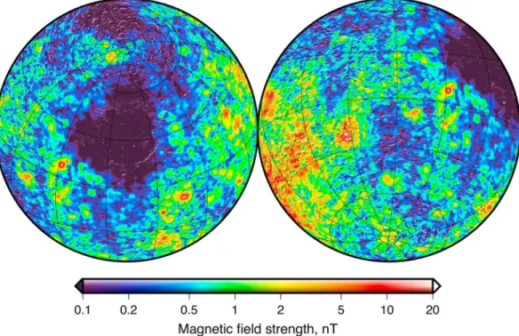
Figure 1. Total magnetic field strength of the Moon at 30 km altitude plotted using a (top) linear and (bottom)
logarithmic color scale. The magnetic field was evaluated using a 449∘and order spherical harmonic expansion of
the model of Tsunakawa et al. (2015). The field strength maps are presented in Lambert azimuthal equal-area projections centered over the (left) nearside and (right) farside hemispheres and are overlain by a shaded relief map derived from
the Lunar Orbiter Laser Altimeter Smith et al. (2010). Grid lines are spaced every 30∘in latitude and longitude.
Another fundamental question concerning lunar magnetism is the origin of the magnetic carriers. Though it is well known that metallic iron alloyed with small quantities of nickel (kamacite) is the primary magnetic mineral in lunar rocks (e.g., Fuller & Cisowski, 1987), this metal could be either of lunar or meteoritic origin. Given that most endogenous crustal rocks have low concentrations of metallic iron, they are incapable of accounting for the strongest crustal magnetic anomalies observed from orbit Wieczorek et al. (2012). Recent studies have thus highlighted the importance of the delivery of metallic iron to the Moon from the projectiles that formed the largest impact basins. In one such study by Wieczorek et al. (2012), hydrocode simulations of the impact process have shown that if the giant farside South Pole-Aitken basin formed under oblique impact conditions, with the projectile traveling from south to north, projectile materials could have been deposited precisely where the largest grouping of farside magnetic anomalies is found. In another study by Oliveira et al. (2017), the impact melt sheets of several Nectarian-aged impact basins (including Mendel-Rydberg, Nectaris, Serenitatis, Humboldtianum, and Crisium) were shown to possess central magnetic anomalies that could be accounted for by small quantities of metallic iron derived from the projectile.
As a result of vectorial magnetic field measurements made from orbit by the Lunar Prospector and Kaguya spacecraft, the global properties of the Moon’s lithospheric magnetic field are now well characterized. The total magnetic field strength of the Moon at 30 km altitude from the model of Tsunakawa et al. (2015) is plotted in Figure 1, which is based on measurements from both missions. The nearside and farside hemi-spheres are plotted on the left and right, respectively, and the upper and lower set of images plot the field
strength using a linear and logarithmic color scale, respectively. As shown in the upper set of images, there are only a few dozen strong anomalies scattered across the lunar surface, and a large grouping of anomalies in the farside highlands. Though a few of these anomalies are associated with impact basins, the vast majority have no known correlation with any lunar geologic process. Many investigations have investigated the strength and direction of magnetization of the strongest and most isolated of these anomalies (e.g., Arkani-Hamed & Boutin, 2014; Blewett et al., 2007; Halekas et al., 2001, 2003; Hemingway & Garrick-Bethell, 2012; Hood, 2011; Hood et al., 2001, 2013; Mitchell et al., 2008; Nayak et al., 2017; Nicholas et al., 2007; Oliveira & Wieczorek, 2017; Oliveira et al., 2017; Purucker et al., 2012; Richmond et al., 2003, 2005; Takahashi et al., 2014; Wieczorek et al., 2012).
When the magnetic field strength is plotted using a linear scale, one could have the impression that only a small portion of the crust of the Moon was ever magnetized. However, when the field strength is plotted using a logarithmic scale, it is evident that magnetic fields are present everywhere and that large portions of the crust must in fact be magnetized. The lowest intensities plotted in this map are not a result of mea-surement noise as the same general tendencies can be seen in the surface field strengths derived from the Lunar Prospector electron reflectometer, which is based on a completely different measurement technique (see Mitchell et al., 2008). These weak, omnipresent crustal fields have not been investigated in any detail, and their origin is thus largely unexplored. In particular, it is not known if the magnetized materials respon-sible for these weak anomalies are located near the surface or if they are instead found deep in the crust. It is not known if the magnetic minerals are derived from endogenous lunar materials, or if they are instead a result of meteoritic contamination. Lastly, it is not known if these anomalies formed early in lunar history when the primordial crust was cooling, or if they formed later as a result of processes related to impact events or crustal magmatism. It is the origin of these weak fields that encompass the Moon that will be the main focus of this work.
To address the origin of lunar crustal magnetism, one would like to know the strength of magnetization in the crust, the geometry of the sources, and the depth range over which the sources reside. With this information, it would be possible to test various hypotheses. For example, if the magnetic sources were all located close to the surface, this might indicate that the sources were delivered to the Moon during impact events. If the sources were instead found deep in the crust, this might suggest that they either formed at the same time as the crust itself or they are related to later magmatic intrusions that cooled within the crust. Furthermore, if there were any variations in the strength of crustal magnetization, this could either be indicative of lateral variations in the abundance of magnetic carriers, or time variations in the strength of the field that magnetized the crust.
These questions will be addressed in this paper by the use of a statistical model of crustal magnetization. It will be assumed that crustal magnetization can be described by ensembles of magnetized sills or prisms, where the locations and magnetization vectors of the sources are both random. As will be shown, it is possible to derive analytic expressions for the power spectrum of the magnetic field that depend upon four parameters that describe the strength, size, and depth range of the magnetic sources. This model is highly inspired by a similar model that was developed by Voorhies (1998) and that was used to interpret the magnetic field of both Earth and Mars. In contrast to the pioneering work of Voorhies et al. (2002) and Voorhies (2008), who analyzed global magnetic power spectra, we will instead perform a localized power spectrum analysis using the techniques developed by Wieczorek and Simons (2005, 2007) to constrain how the model parameters vary across the surface of the Moon. A similar application of this approach applied to Mars can be found in Lewis and Simons (2012).
Our analysis comprises several steps. In section 2, the mathematical relations needed for a power spectrum analysis of a global magnetic field are provided. Two stochastic models of crustal magnetization are then developed that predict the global power spectrum, where one consists of ensembles of magnetized prisms and the other of magnetized sills. The properties of these two models are then explored and contrasted. In section 3, the technique of using a localized power spectrum analysis to invert for model parameters is described. This includes the construction of localization windows and a description of the manner by which both the data and model are localized. Furthermore, a Monte Carlo technique for placing confidence limits on the inversion parameters is described. In section 4, we perform a localized spectrum analysis of the Moon’s magnetic field and invert for model parameters. Next, in section 5 we discuss two aspects of our model results. First, we describe how the size, geometry, and depth of sources constrain the origin and timing of crustal
A
B
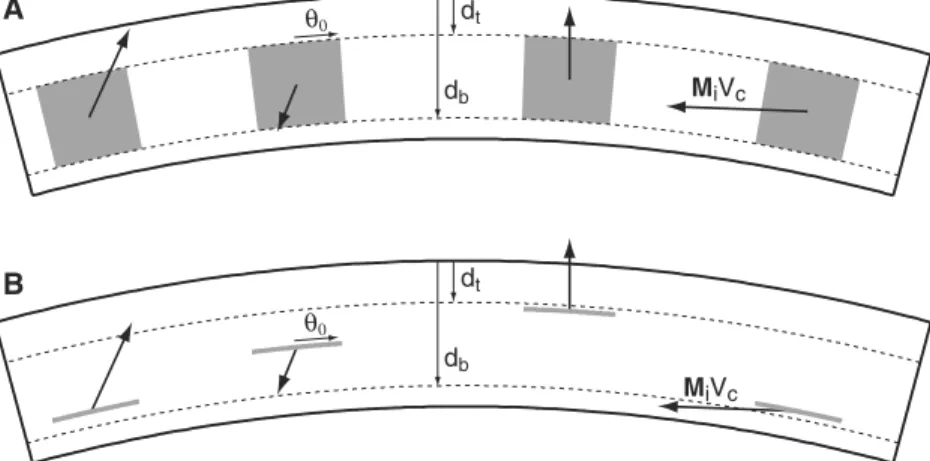
MiVc dt db θ0 dt db MiVc θ0Figure 2. Schematic diagram of the stochastic model of crustal magnetization used in the magnetic field power
spectrum analysis. (a) The magnetization is confined to a series of thick spherical prisms, each possessing the same
volumeVc, the same angular radius𝜃0, and the same depths to the top and bottom of magnetization,dtanddb,
respectively. A spherical prism is here defined to be a cone with its apex at the center of the planet that is truncated
by two spheres of different radii. The magnetization vectorsMiare random, as are the locations of each cap. (b) The
magnetization is confined to a series of thin spherical caps with total magnetic momentMiVc, and each cap is located
randomly in the shell between the depthsdtanddb.
magnetization. Second, we discuss the origin of a region of crust on the nearside that has extremely weak magnetization and field strengths. Finally, we conclude in section 6 by discussing some questions that remain unresolved and by providing guidance for future directions of research.
2. Stochastic Power Spectrum Models
The objective of this section is to calculate the theoretical power spectrum that results from a statistical collection of magnetized regions in a planetary body. This problem was studied previously by several authors. Voorhies, (1998, 2008) and Voorhies et al. (2002) gave expressions for the power spectrum when the magne-tized regions were spatially uncorrelated dipoles in a spherical or ellipsoidal shell, depth correlated dipoles, or infinitesimally thin radially magnetized spherical caps. Jackson (1990, 1994) gave expressions for the case where the distribution of magnetization could be described by a lateral and vertical spatial correlation function. Bouligand et al. (2009) made use of a fractal model of magnetization whose Cartesian power spectrum was described by a power law in order to invert for the depth of magnetization on Earth. In a study by Thébault and Vervelidou (2015), the power spectrum of laterally varying magnetic susceptibility was assumed to follow a power law, which allowed to predict the magnetic power spectrum of the field induced by a central dipole. This technique was applied to Earth by Vervelidou and Thébault (2015) to invert for the thickness of the magnetic layer.
For the Moon, there are presently no fields generated by a core dynamo, and the observed static magnetic field is due entirely to magnetization in its lithosphere. To describe the observed magnetic power spectrum, two theoretical models will be developed that expand upon and generalize the results of Voorhies et al. (2002). The first model assumes that the power spectrum of the magnetic field can be approximated by that due to an ensemble of thick magnetized spherical prisms, each of which possesses a random lateral position, random volumetric magnetization, and random magnetization direction (model A in Figure 2). The fixed parameters of this model include the angular radius of the spherical prisms, a parameter that depends on the mean-squared dipole moment, and the depth to the top and bottom of the magnetized region. The second model is a gen-eralization of the first and accounts for the case of thin magnetized caps (referred to below as sills) that are placed randomly within a thick spherical shell (model B in Figure 2). Both of these generic models are consis-tent with the functional forms given in Jackson (1994). Furthermore, these models reduce to the equations given in Voorhies et al. (2002) for their special cases of crustal magnetism. In particular, our model can account for their model of random dipoles placed within a finite thickness shell, vertically correlated dipoles within a finite thickness shell, and thin magnetized spherical caps. In contrast, we note that Voorhies et al. (2002) did not provide equations for vertically correlated spherical caps (our model A), nor uncorrelated spherical caps within a finite layer (our model B). Since the magnetic field of a uniformly magnetized sphere is equivalent
to that of a single dipole in the center of this sphere, our magnetic power spectrum models also account implicitly for uniformly magnetized spheres as well.
In the first subsection, definitions of the magnetic potential, power spectrum, and spherical harmonic nor-malizations are provided that are required for the analysis. The theoretical power spectrum is then derived for the two classes of magnetization that are shown in Figure 2. Following these derivations, the properties of their power spectra are described and compared.
2.1. Definitions
In the absence of free currents and time-variable electric fields, the curl of the magnetic field B is zero. This allows B to be expressed as the gradient of a scalar potential
B(r) = −∇U(r) (1)
that can be calculated explicitly via a surface and volume integral over the distribution of magnetization (e.g., Blakely, 1995, equation 5.4) U(r′) = 𝜇0 4𝜋 ∫S M(r)⋅ da |r′− r| − 𝜇0 4𝜋 ∫V ∇⋅ M(r) dV |r′− r| , (2)
where M is the dipole moment per unit volume (in units of A m−1) within the volume V enclosed by the surface S, da is the differential surface area with direction normal to the surface, and𝜇0is the magnetic constant, 4𝜋 × 10−7T m A−1. As a solution to Laplace’s equation, the potential can be expanded exterior to the magnetized
sources as a weighted sum of spherical harmonic functions
U(r) = a L ∑ l=1 l ∑ m=−l (a r )l+1 glmYlm(𝜃, 𝜙), (3)
where Ylmis a spherical harmonic function of degree l and order m as a function of colatitude𝜃 and longitude
𝜙, glmis the corresponding spherical harmonic Gauss coefficient (in units of teslas) evaluated at radius a, and
Lis the maximum spherical harmonic degree of the expansion. The real spherical harmonic functions are defined by
Ylm(𝜃, 𝜙) =
{ ̄Plm(cos𝜃) cos m𝜙 if m≥ 0
̄Pl|m|(cos𝜃) sin |m|𝜙 if m < 0, (4)
where the Schmidt seminormalized associated Legendre functions ̄Plm are related to the unnormalized
functions, both of which exclude the Condon-Shortley phase of (−1)m, by
̄Plm(x) =
√
(2 −𝛿0m)(l − m)!
(l + m)!Plm(x), (5)
where x = cos𝜃, and where 𝛿 is the Kronecker delta function. With these definitions, the spherical harmonics are orthogonal over the sphere and possess the normalization
∫Ω
Ylm(𝜃, 𝜙) Yl′m′(𝜃, 𝜙) dΩ = 4𝜋
(2l + 1)𝛿ll′𝛿mm′, (6) where dΩ = sin𝜃 d𝜃 d𝜙. If the coefficients glmare initially referenced to a radius a, as in equation (3), the
corresponding coefficients referenced to a′can be shown to be given by g(alm′)= glm
(a
a′
)l+2
. (7)
Later, for the localized spectral analyses, it will be necessary to make use of 4𝜋-normalized harmonics, which are defined by
∫Ω
Ylm(4𝜋)(𝜃, 𝜙) Yl(4′m𝜋)′(𝜃, 𝜙) dΩ = 4𝜋 𝛿ll′𝛿mm′. (8)
It is easily shown that Schmidt-seminormalized and 4𝜋-normalized spherical harmonic coefficients are related by the expression
g(4lm𝜋)= √glm 2l + 1.
The total power of the magnetic potential at the reference radius a is 1 4𝜋 ∫Ω U(a, 𝜃, 𝜙)2dΩ = L ∑ l=1 SU(l), (10)
where the power spectrum S is
SU(l) = a2 (2l + 1) l ∑ m=−l g2lm= a2 l ∑ m=−l ( g(4lm𝜋))2. (11)
Similarly, the total power of the magnetic field at radius r can be shown (after a somewhat complicated derivation) to be 1 4𝜋 ∫ΩB(r)⋅ B(r) dΩ = L ∑ l=1 SB(l, r), (12)
where the Lowes-Mauersberger power spectrum of the magnetic intensity is (e.g., Lowes, 1966)
SB(l, r) = (a∕r)2l+4(l + 1) l ∑ m=−l g2 lm, = (a∕r)2l+4(l + 1)(2l + 1) SU(l)∕a2. (13)
For ease of notation, the radius at which the power spectrum is calculated will not be indicated when it is equal to the reference radius of the coefficients a. In the geomagnetism community, SBis commonly denoted by the
symbol R. If it is assumed that the coefficients glmare independent Gaussian random variables with zero mean,
and that the variance of the coefficients depends only upon degree l, then it can be shown (see Wieczorek & Simons, 2007, appendix C) that the variances of the magnetic potential and magnetic power spectra are
var{SU(l)}= 2 (2l + 1)⟨SU(l)⟩ 2, (14) var{SB(l) } = 2 (2l + 1)⟨SB(l)⟩ 2, (15)
where the operator⟨· · ·⟩ denotes an ensemble average over the random variables.
2.2. Magnetized Prisms
We start by calculating the Gauss coefficients of a single uniformly magnetized spherical prism of angular radius𝜃0with upper and lower bounding radii r+and r−, respectively (see Figure 2a). A spherical prism is here
defined to be a cone with its apex at the center of the planet that is truncated by two spheres of different radii. For our inversions later in this paper, for convenience, the bounding radii will be expressed in terms of the depth to the top and bottom of the magnetized region, dtand db, respectively. Since we are concerned primarily with calculating the power spectrum of the magnetic field, and since the power spectrum is invariant under a rotation of the coordinate system, with no loss of generality, we can place the center of the spherical cap at𝜃 = 0.
If the magnetization in the cap is constant in direction
M = Mx̂x + Mŷy + Mẑz, (16)
then both the divergence of M and the volume integral in equation (2) are identically zero. By calculating a surface integral over the prism, the Gauss coefficients can be shown to be equal to (see Appendix A)
glm= 𝜇0 2 [(r+ a )l+2 −( r− a )l+2] × [ 1 2 ( 𝛿m1Mx+𝛿m,−1My ) ( ∫ 1 cos𝜃0 ̄Pl1(x) ̄P11(x) dx +
̄Pl1(cos𝜃0) sin𝜃0cos𝜃0 (l + 2) ) +𝛿m0Mz ( ∫ 1 cos𝜃0 ̄Pl0(x) ̄P10(x) dx − ̄Pl0(cos𝜃0) sin2𝜃0 (l + 2) )] . (17)
The coefficients for a magnetized spherical prism centered at any arbitrary location could be obtained using standard spherical harmonic rotation algorithms (e.g., Blanco et al., 1997; Varshalovich et al., 1988).
We next make the assumption that the planet contains N magnetized spherical prisms, all of the same size
𝜃0and all with the same bounding radii r+and r−. The Gauss coefficients for the ensemble of these prisms
are simply ̃glm= N ∑ n=1 g(n)lm (18)
where g(n)lmare the coefficients of the nth prism centered at (𝜃n, 𝜙n). If the position, volumetric magnetization,
and magnetization direction of each prism are all random, the expectation of the power spectrum at radius
ais ⟨SB(l)⟩ = (l + 1) ⟨ l ∑ m=−l N ∑ i=1 N ∑ j=1 g(i)lmg(j)lm ⟩ . (19)
The expectation of the product of the two coefficients is zero when i≠ j, and since the power for an individual prism at degree l is unchanged by a rotation of coordinates, the power spectrum is simply N times the power of a single prism ⟨SB(l)⟩ = N (l + 1) ⟨ l ∑ m=−l g2lm ⟩ . (20)
Given the assumption of random volumetric magnetizations and magnetization directions, we have ⟨MxMy⟩ = ⟨MxMz⟩ = ⟨MyMz⟩ = 0, (21) and ⟨M2 x⟩ = ⟨M 2 y⟩ = ⟨M 2 z⟩ = ⟨M 2⟩∕3, (22)
where⟨M2⟩ is the average squared magnetization in the prisms. Using these equations to calculate the
expec-tation of the square of equation (17), the expecexpec-tation value of the power spectrum can be shown to be given by ⟨SB(l)⟩ = N ⟨M2⟩ Z p l ( 𝜃0, r+, r−, a ) , (23)
where we have introduced for convenience the function Zp that contains all terms related to the source
geometry and volume, and where the superscript denotes that this is for the model of composed of prisms:
Zlp(𝜃0, r+, r−, a ) =𝜇 2 0(l + 1) 12 [(r+ a )l+2 −( r− a )l+2]2 × [ 1 2 ( ∫ 1 cos𝜃0 ̄Pl1(x) ̄P11(x) dx +
̄Pl1(cos𝜃0) sin𝜃0cos𝜃0
(l + 2) )2 + ( ∫ 1 cos𝜃0 ̄Pl0(x) ̄P10(x) dx − ̄Pl0(cos𝜃0) sin2𝜃0 (l + 2) )2] . (24)
In practice, it will be more convenient to solve for a quantity related to the magnetic moment (in units of A m2) as opposed to the magnetization M. This is because there will be a partial trade-off between the chosen
magnetization and the volume of the magnetized region, with the volume dependence being accounted for in the function Z. Multiplying and dividing equation (23) by the volume-squared of the prism yields
⟨SB(l)⟩ = N ⟨M2⟩ Vp2 ⎧ ⎪ ⎨ ⎪ ⎩ Zlp(𝜃0, r+, r−, a )( 3 2𝜋 (r3 +− r−3) (1 − cos𝜃0) )2⎫ ⎪ ⎬ ⎪ ⎭ , (25)
where the volume of a single prism is given explicitly by Vp=2𝜋 3 ( r3 +− r 3 − ) ( 1 − cos𝜃0). (26)
As shown in Appendix B, the integrals of the associated Legendre functions in equation (24) can be expressed in terms of the first derivatives of ordinary Legendre polynomials. Using the power spectrum for a prism of a specific size, it is straightforward to derive the predicted power spectrum for a given size-frequency distribution of prisms.
2.3. Magnetized Sills
A related model for the magnetic power spectrum of a planet is to assume that the observed spectrum is the result of many thin spherical caps that are each magnetized in a random direction and that are randomly distributed in the volume between radii r+and r− (see Figure 2b). Such thin caps could be thought of as magmatic sills. We start by generalizing the power spectrum of N spherical prisms from equation (23) to that of a single thin cap at radius rxwith a finite, but small, thickness d. When r+and r−approach rxit is easily
shown that ⟨SB(l, rx)⟩ =𝜇20⟨M 2⟩(l + 1)(l + 2)2 12 (d a )2( r x a )2l+2 × [ 1 2 ( ∫ 1 cos𝜃0 ̄Pl1(x) ̄P11(x) dx +
̄Pl1(cos𝜃0) sin𝜃0cos𝜃0
(l + 2) )2 + ( ∫ 1 cos𝜃0 ̄Pl0(x) ̄P10(x) dx − ̄Pl0(cos𝜃0) sin2𝜃0 (l + 2) )2] . (27)
If N sills are located randomly within a volume V defined by upper and lower radii r+and r−, such that the spatial density of sills is simply N∕V, the total power spectrum can be calculated as
⟨SB(l)⟩ = N V ∫ r+ r− ∫Ω SB(l, rx) r2xdrxdΩ, (28) where V =4𝜋 3 ( r3 +− r 3 − ) . (29)
At this point, two possible assumptions could be made about the sills: either the volume of the sills or the thickness of the sills could be considered constant. The two scenarios are nearly identical from a numerical point of view, but the constant thickness sill solution is more amenable to analysis when there is a distribution of sill sizes. Here we make the assumption that the sill thickness d is constant and present the results for constant volume sills in Appendix C. Integrating equation (28), the power spectrum is shown easily to be
⟨SB(l)⟩ = N ⟨M2⟩ Zsl ( 𝜃0, r+, r−, a ) , (30) where Zs l ( 𝜃0, r+, r−, a ) =𝜇 2 0d 2a𝜋 3 V (l + 1)(l + 2)2 (2l + 5) [(r+ a )2l+5 −( r− a )2l+5] × [ 1 2 ( ∫ 1 cos𝜃0 ̄Pl1(x) ̄P11(x) dx +
̄Pl1(cos𝜃0) sin𝜃0cos𝜃0
(l + 2) )2 + ( ∫ 1 cos𝜃0 ̄Pl0(x) ̄P10(x) dx − ̄Pl0(cos𝜃0) sin2𝜃0 (l + 2) )2] , (31)
10−5 10−4 10−3 10−2 10−1 100 101 Power, nT 2 θ0=0.01°, dt=0, db=10 km θ0=0.1°, dt=0, db=10 km θ0=0.5°, dt=0, db=10 km θ0=1°, dt=0, db=10 km 10−5 10−4 10−3 10−2 10−1 100 101 Power, nT 2 θ0=0.1°, dt=0, db=30 km θ0=0.1°, dt=5 km, db=30 km θ0=0.1°, dt=10 km, db=30 km θ0=0.1°, dt=20km, db=30 km 10−5 10−4 10−3 10−2 10−1 100 101 Power, nT 2 0 50 100 150 200 250 300 350 400 450 0 50 100 150 200 250 300 350 400 450 0 50 100 150 200 250 300 350 400 450 Spherical harmonic degree
θ0=0.1°, dt=0, db=10 km
θ0=0.1°, dt=0, db=20 km
θ0=0.1°, dt=0, db=30 km
θ0=0.1°, dt=0, db=40 km
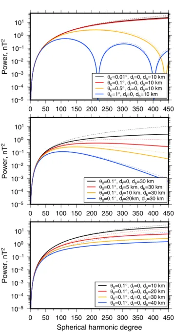
Figure 3. Example power spectra for ensembles of magnetized prisms
(solid lines) and sills (thin dashed lines). (top) Dependence of the power
spectrum on the angular radius𝜃0of the magnetized sources (1∘is
∼30 km on the lunar surface). All magnetized sources are placed
between the surface and 10 km depth. (middle) Dependence of the power spectrum on the depth to the top of the magnetized region.
The depth to the bottom of the magnetized region is 30 km, and𝜃0
is 0.1∘. (bottom) Dependence of the power spectrum on the depth to
the bottom of the magnetized region. The top of the magnetized
region is located at the surface and𝜃0is 0.1∘.
and where the superscript s denotes that this is for the model composed of sills. Multiplying and dividing equation (30) by the volume squared of the sills yields ⟨SB(l)⟩ = N ⟨M2⟩ Vs2 ⎧ ⎪ ⎨ ⎪ ⎩ Zls(𝜃0, r+, r−, a )( 5 (r3 +− r3−) 6𝜋 d (r5 +− r−5) (1 − cos𝜃0) )2⎫ ⎪ ⎬ ⎪ ⎭ , (32) where the average volume of a sill of constant thickness and angular radius
𝜃0is Vs= 6𝜋 d 5 ( r5 +− r 5 − ) ( r3 +− r−3 ) (1 − cos 𝜃0). (33)
It is noted that the last term in brackets of equation (32) does not depend upon the sill thickness d, as the reciprocal of d−2is found in the function Zs.
2.4. Example Power Spectra
The model power spectra for randomly magnetized prisms and sills are very similar in form. As seen in equations (25) and (32), the spectra depend upon a multiplicative prefactor N⟨M2⟩V2that is the total number of sources
multi-plied by their mean-squared dipole moment, and a degree-dependent term
Zthat depends upon the geometry of the sources. The geometric function Z is composed further of two multiplicative terms, one that depends solely on the radii over which the sources reside and another that depends solely on the angular size of the sources. Given the nature of the prefactor N⟨M2⟩V2,
it will not be possible to invert individually for the number of sources, their magnetization, or their dipole moment, as they are all correlated.
The three terms that control the form of the geometric factor Z are the depth to the top of the magnetized region dt, the depth to the bottom of the
mag-netized region db, and the angular radius of the sources𝜃0. The dependence
of the model spectrum on these terms is illustrated in Figure 3, where the top panel shows how the magnetic power spectrum varies as a function of the angular size of the sources, the middle panel shows how the spectra vary as a function of the depth to the top of the magnetized region, and the bottom panel shows the dependence on the depth to the bottom of the magnetized region. The maximum spherical harmonic degree plotted is 450, which cor-responds to the maximum resolution of the lunar magnetic field that will be employed later.
In Figure 3 (top), spectra are plotted for several values of 𝜃0 from 0.01∘ (∼30 m) to 1∘ (∼30 km), with dtand dbset to constant values of 0 and 10 km, respectively. It is first noted that the model spectra for magnetized sills and prisms are nearly identical for degrees less than about 150. For higher degrees, the power is slightly larger for magnetized sills than for magnetized prisms. For both models, the majority of the power is found to reside in the first spec-tral lobe, which empirically is found to have a bandwidth of about 1.2×180∕𝜃0,
with𝜃0in degrees. The spectral lobes are a result of the fact that the
magne-tized regions have a finite width with sharp boundaries. Each successive lobe has a lower maximum amplitude, and for the smallest values of𝜃0 plotted (0.01∘ and 0.1∘), only a portion of the first lobe is visible. As𝜃0
approaches zero, the spectra are seen to converge rapidly to an asymptotic form.
In Figure 3 (middle), spectra are plotted for several values of the depth to the top of the magnetized region, from 0 to 20 km. Here the depth to the bottom of the sources was set to 30 km, which is slightly smaller than the average thickness of the lunar crust (e.g., Wieczorek et al., 2013), and the angular radius of the sources was set to 0.1∘. The depth to the top of the sources is seen to have a major influence on the spectra at the
10−5 10−4 10−3 10−2 10−1 100 101 Power, nT 2 0 50 100 150 200 250 300 350 400 450 Spherical harmonic degree
Random magnetization Radial magnetization Horizontal magnetization
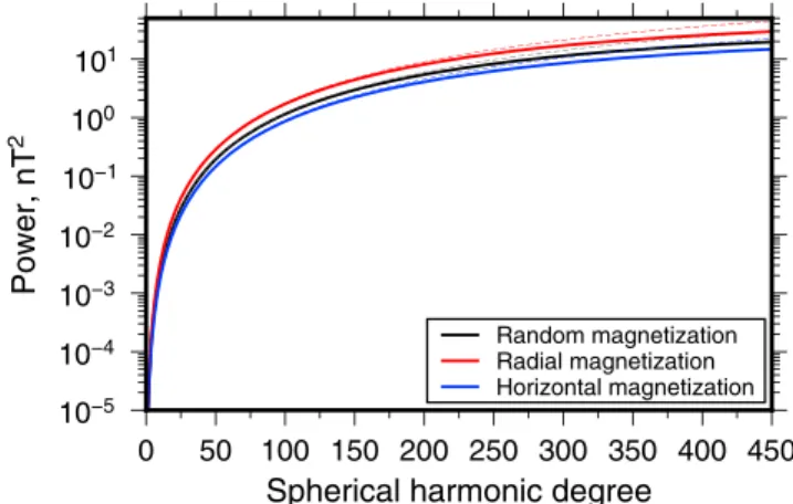
Figure 4. Dependence of the magnetic power spectrum on the
direction of magnetization for ensembles of prisms (solid lines) and sills (thin dashed lines). Black curves correspond to the case where the magnetization directions are random, whereas the red and blue curves correspond to the cases where the sources are all magnetized in either the radial or horizontal directions, respectively. All magnetized sources are placed between the surface and 10 km depth, and the
angular radius𝜃0of the sources is 0.1∘.
highest degrees. As the depth to the top of the sources increases, the high-degree power decreases. This behavior is easily understood from the math-ematical form of the geometric function Z in equations (24) and (31), and suggests that this value will be constrained easily from observations. Figure 3 (bottom) demonstrates how the magnetic power spectrum depends upon the depth to the bottom of the magnetized sources. In this example, the angular radius of the sources was set to 0.1∘, the top of the magnetic sources was set to the surface, and the depth of the sources was varied from 10 to 40 km. For most of the degree range that is plotted, the spectra all have some-what similar slopes, especially for degrees greater than about 100. Beyond this degree, the spectra are approximately offset only by a vertical scaling fac-tor. This behavior suggest that it will be difficult to invert for the depth to the bottom of the magnetized region as this will partially trade off with the factor
N⟨M2⟩V2that multiplies each of these curves.
Finally, we consider how the direction of magnetization affects the model power spectra. Up until this point, we have treated the case where the direc-tion of magnetizadirec-tion of each individual source was random. This assumpdirec-tion provided a simple expression for the expectation of the magnetization vector in each orthogonal direction as given by equation (22), as well as zero values for the cross expectation of two components in equation (21). An alternative model might be to instead assume that all magnetic sources were magne-tized in the same direction. We quantify how the magnetic power spectrum for this case differs from that of random magnetization by considering two end-member cases: horizontally magnetized sources and radially magnetized sources.
The derivations for these models are nearly identical to those presented earlier in this section, and only dif-fer by setting M = Mx̂x for horizontally magnetized sources and M = Mẑz for vertically magnetized sources.
In Figure 4 we plot these two models in blue and red, respectively. The power spectrum for the case of radi-ally magnetized sources is found to be always about 2 times larger than the case of horizontradi-ally magnetized sources. As these two curves are very similar to our model with random magnetization directions, which lies between the two end-members, we do not expect the results of our inversion to depend sensitively on the actual direction of magnetization. This factor of 2 difference will simply become incorporated into the prefactor N⟨M2⟩V2.
3. Localized Spectrum Analysis
A stochastic model consisting of randomly magnetized prisms or sills was developed in section 2 that predicts the expected global magnetic power spectrum of a planet. This model assumes implicitly that the proper-ties of the magnetic sources are globally uniform and do not vary from place to place. In reality, as a result of lateral variations in geologic processes (such as variations in crustal cooling rates and variations in the abundance of the magnetic carriers), one might expect that the model parameters should also vary as a func-tion of posifunc-tion. To quantify such lateral variafunc-tions, instead of inverting the observed global magnetic power spectrum for best fitting model parameters, we will perform a localized multitaper power spectrum analysis that extracts the spectral properties of the magnetic field over prescribed regions. In this section, we describe the methodology used in this analysis, which includes the construction of a global spherical harmonic model of the Moon’s magnetic field based on the gridded data of Tsunakawa et al. (2015), the construction of spa-tiospectral localization windows for the multitaper spectrum analyses, the inversion of the localized spectra for model parameters, and Monte Carlo techniques for estimating the uncertainties of the model parameters. We first develop a global spherical harmonic model of the Moon’s magnetic field that is based on the global 0.2∘ gridded map of the radial component of the magnetic field developed by Tsunakawa et al. (2015). This model is based on a combination of vector magnetic field measurements from the Kaguya and Lunar Prospec-tor spacecraft, and after a global model for the radial field was constructed, Tsunakawa et al. (2015) were able to derive maps of the other two horizontal components directly from their radial field map. The gridded model of the radial field thus contains all the information in their model. Using the software package SHTOOLS (Wieczorek et al., 2016), the spherical harmonic coefficients of the radial magnetic field were calculated,
10−4 10−3 10−2 10−1 100 Power, nT 2 0 50 100 150 200 250 300 350 400 450 Spherical harmonic degree
Tsunakawa et al. (2015)
Purucker and Nicholas 2010 (sequential) Purucker and Nicholas 2010 (coestimation) Purucker and Nicholas 2010 (correlative)
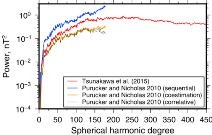
Figure 5. Magnetic power spectra of the Moon. The power spectrum
of the model developed by Tsunakawa et al. (2015) is based on measurements obtained by the Kaguya and Lunar Prospector spacecraft, whereas the three models of Purucker and Nicholas (2010) are based exclusively on measurements from Lunar Prospector. The power is calculated at a radius of 1,737.4 km.
and the Gauss coefficients of the magnetic potential were then obtained by dividing these by (l + 1) (cf. equation (3). The final spherical harmonic model is developed up to degree 449, which is the maximum degree allowed by the Driscoll and Healy (1994) sampling theorem.
The magnetic field intensity of the Tsunakawa et al. (2015) model was shown previously in map form in Figure 1, and here we plot in Figure 5 the mag-netic power spectrum of this model. The form of the power spectrum is similar in many respects to that of the model spectrum developed in section 2. The power is low at the lowest degrees and then increases several orders of mag-nitude over the first 100 degrees. The power then increases more slowly to achieve a broad peak close to degree 200 and then decreases slightly and continues with a nearly constant value after about degree 350. Also plotted are the power spectra of three different global models developed by Purucker and Nicholas (2010) that were based solely on Lunar Prospector data. These models have a lower spatial resolution than the Tsunakawa et al. (2015) model, with a maximum spherical harmonic degree of 180. Furthermore, it is seen that the power spectra of the three Purucker and Nicholas (2010) models dif-fer by about a factor of 5, which they interpreted to be a result of the strong regularization applied to their “coestimation” model. The power spectrum of the Tsunakawa et al. (2015) model lies about halfway between the “sequential” and “coestimation” models of Purucker and Nicholas (2010).
To obtain estimates of the magnetic power spectrum localized to a prescribed region of interest, we use the multitaper spectrum analysis technique as developed in spherical geometry for scalar fields by Wieczorek and Simons (2005, 2007). The technique is conceptually very simple: Several orthogonal windows of prescribed spherical harmonic bandwidth are constructed that localize optimally their energy in a spherical cap of spec-ified angular radius, the localization window is rotated to the region of interest, the data are multiplied by the window, the resulting function is expanded in spherical harmonics, and the power spectrum of the localized function is computed. The multitaper spectrum estimate is defined as the average of the spectra from each of the individual localization windows. By using several orthogonal localization windows, statistical fluctuations associated with the underlying process are reduced, which provides a better estimate of the power spectrum expectation of the process. The uncertainty in the multitaper spectrum estimates decreases as 1∕√K, where
Kis the number of localization windows (Wieczorek & Simons, 2007, equation 4.4). All of these computations are readily performed by routines in the SHTOOLS software package.
Only minor modifications to this method are required when applying a multitaper spectrum analysis to magnetic field data (see also Lewis & Simons, 2012). First, we convert the Schmidt seminormalized Gauss coef-ficients to 4𝜋-normalized coefficients using equation (9) in order to be compatible with the normalization used by the localization windows. Second, we localize the magnetic potential (not the vector components) and then convert the localized spectrum of the potential to a localized power spectrum of the magnetic field by multiplying by (2l + 1)(l + 1)∕a2(see equation (13)). At this point, all that is left to do is to choose the size
and the spectral bandwidth Lwinof the window: these two quantities determine how many windows will be
well localized. We note that it is desirable that the spectral bandwidth of the windows be as small as possible, since the localized spectrum can be interpreted only between Lwinand L − Lwin, where L is here 449. On the
low-degree end, this limitation is a result of the fact that it is not possible to resolve wavelengths that are greater than the size of the localization region. On the high-degree end, this limitation arises because the local-ized spectrum at degrees greater than L − Lwindepends upon global spherical harmonic model coefficients
beyond what are available. As Lwinincreases, the number of windows that are well localized increases, the
uncertainty associated with the multitaper spectrum estimate decreases, and the degree range over which the localized power spectrum can be interpreted decreases. Alternative localization techniques that make use of vectorial fields can be found in Thébault et al. (2006) and Plattner and Simons (2017).
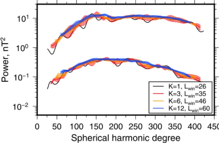
As an illustrative example, we chose the size of the localization region to be a spherical cap with an angular radius of 10∘ and then chose the spectral bandwidth of the windows to be 26, 35, 46, and 60. Using the criteria that a window is well localized if 99% of its power is concentrated in the region of interest, these bandwidths provide 1, 3, 6, and 12 windows that are well localized. Figure 6 plots the localized magnetic power spectra
10−2 10−1 100 101 Power, nT 2 0 50 100 150 200 250 300 350 400 450 Spherical harmonic degree
K=1, Lwin=26
K=3, Lwin=35
K=6, Lwin=46
K=12, Lwin=60
Figure 6. Example localized magnetic power spectra using windows
with an angular radius of 10∘. The localized spectra were calculated over
two representative regions on the farside: a high field strength region
at (30∘S, 170∘E) and a medium field strength region at (15∘S, 120∘E).
The number of well-localized tapersKfor the specified spectral
bandwidth of the window varies from 1 to 12 and the plotted error bars correspond to the standard error of the multitaper estimate.
using these four sets of windows for two regions on the farside of the Moon, one that has high field strengths in the northern portion of the South Pole-Aitken basin and another with low field strengths to the northwest of this basin. The spectra of the two regions are similar in form and differ primarily by a multiplicative constant, reflecting different strengths of magnetization in the crust. As is seen, when a single localization window is used (black lines), the spectrum possesses substantial oscillations, but as more and more win-dows are employed, the multitaper spectrum estimate becomes progressively smoother. The uncertainty of the spectral estimates decreases with the num-ber of windows, and as expected, the uncertainty using 12 windows is about 2 times smaller than when using 3 windows. As the number of well-localized windows increases, the bandwidth of the windows also increases, which reduces the range of spherical harmonic degrees that can be interpreted. When a global function is multiplied by a localization window, the power spectrum of the localized function will differ naturally from that of the global function. Thus, when comparing localized spectra of the observed magnetic field to a model, it is important that these be compared to models that are localized in a similar manner. In many geophysical analyses, such as when ana-lyzing the relation between gravity and topography (e.g., Besserer et al., 2014), it is possible to construct a forward model of the field that is then localized in exactly the same manner as the data. In our case, though, the magnetization model is inherently statistical in nature, and the generation of individual forward models would be somewhat more cumbersome. Fortunately, a relationship does exist that relates the statistical expectation of the local-ized multitaper spectrum estimate to the power spectra of the global field and window (Wieczorek & Simons, 2005, 2007). In particular, for a global scalar function f and a set of localization windows h(k), the expectation
of the multitaper power spectrum of the localized field Φ is ⟨ S(mt)ΦΦ(l) ⟩ = Lwin ∑ j=0 (K ∑ k=1 akS(k)hh(j) ) l+j ∑ i=|l−j| Sff(i) ( Cl0 j0i0 )2 , (34)
where the symbol C is a Clebsch-Gordan coefficient, Shhand Sffare respectively the power spectrum of the window h and function f , and akare the weights used in constructing the multitaper estimate. For this study,
ak will be set equal to 1∕K. The derivation of this equation makes only the assumption that the spherical harmonic coefficients of the function f are zero-mean random variables, and that the coefficients are isotropic, with the variance depending solely on spherical harmonic degree.
When inverting the observed localized magnetic power spectra for model parameters, the goodness of fit between the observations and model will be quantified by a reduced𝜒2function. This misfit function depends
upon the four parameters of our model, N⟨M2⟩V2, d
t, db, and𝜃0, and is given explicitly by
𝜒2 𝜈 ( N⟨M2⟩V2, d t, db, 𝜃0 ) =1 𝜈 L−L∑win l=Lwin ( S(mt)B (l) − S(mt)B (l; N⟨M2⟩V2, d t, db, 𝜃0 ) 𝜎(mt)(l) )2 , (35)
where𝜈 is the number of degrees of freedom that is equal to L−2Lwin− 4, the first two terms in the numerator are respectively the observed multitaper power spectrum and the localized version of the model calculated from equation (34), and𝜎(mt)is the uncertainty associated with the observed multitaper power spectrum,
which is simply the standard error of the K windowed power spectra. The best fitting model parameters will be obtained by sampling the entire model space using an exhaustive grid search.
The 1𝜎 uncertainties on the inversion parameters will be estimated by using a criterion for the maximum allowable misfit that comes from Monte Carlo simulations. To determine this maximum allowable misfit, a global model power spectrum of the magnetic potential is first calculated that corresponds to a set of rep-resentative model parameters. Tests using different model parameters show that the final uncertainties are insensitive to the exact values chosen. Assuming that the spherical harmonic coefficients of the magnetic potential are random variables, which is consistent with the assumptions of our stochastic model, the Gauss coefficients were set to Gaussian random deviates with variance given by equation (14). By definition, this
ensures that the expectation of the magnetic power spectrum is equal to that of the global model. Next, a localized analysis is performed on the simulated Gauss coefficients, and the best fitting model parameters are determined by minimizing the𝜒2
𝜈 function of equation (35). The best fitting𝜒𝜈2is saved, and the entire
procedure is repeated using a new set of Gaussian deviates for the coefficients of the magnetic potential. The cumulative probability distribution P(𝜒2
𝜈) is computed, and the value of𝜒𝜈2where P(𝜒𝜈2) is equal to 68.2%
is ultimately used as the maximum allowable misfit . This misfit defines the 68.2% confidence intervals for the inversion parameters, which determines the 1-𝜎 uncertainties with respect to the best fitting value.
4. Results
A localized spectral analysis and inversion for model parameters was performed at each point on an equally spaced grid that covered the lunar surface with a 5∘ grid spacing at the equator. At each location, the mag-netic potential coefficients were downward continued to the mean elevation of the analysis region using the global topographic map of Smith et al. (2010), and the depths to the top and bottom of the magnetized region were referenced to this datum. The localization analyses made use of windows with an angular radii of 8∘ (a diameter of about 480 km) and spectral bandwidths of 58, which yielded six well-localized windows. The localized spectrum was analyzed from degree 58 to 391, and the misfit was calculated by an exhaustive grid search of the four-parameter model space. As will be discussed at the end of this section, the results were found to be insensitive to variations in the degree range of the localized spectrum that was analyzed and to variations in the localization window parameters.
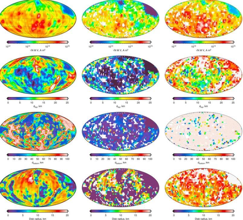
We start by discussing the inversion results using the magnetic power spectrum model that consists of magne-tized sills (the results of the model using prisms are very similar). In Figure 7 are plotted from top to bottom the results for the square root of N⟨M2⟩V2, the depth to the top of the magnetized region, the depth to the bottom
of the magnetized region, and the sill radius. From left to right are plotted the best fitting values interpolated over the entire surface, and the 1𝜎 lower and upper limits of the model parameters. For the uncertainties, individual points are plotted only when the misfit is below the maximum value expected for the 68% con-fidence limit. As expected, about 74% of the analyses can be fit by the model to within the 68% confi-dence limit.
The results for the square root of the parameter N⟨M2⟩V2 (in units of A m2) are perhaps the easiest to
interpret. This parameter is a measure of the number of magnetized sills in the crust, their magnetization, and the sill volume. The best fitting values for this parameter vary over about 3 orders of magnitude, and the lateral variations in this parameter are broadly similar to those seen in the observed magnetic field intensity as plot-ted in the lower portion of Figure 1. Magnetic field strength is thus, unsurprisingly, largely correlaplot-ted with the number of magnetized sills in the crust, and/or their magnetization. As seen in this map, there are two regions that have exceedingly weak magnetizations: one prominent region on the nearside in the region of the Imbrium basin and Oceanus Procellarum and a second smaller region on the northern farside highlands. Each of these regions has prominent magnetic lows in the total magnetic intensity. This map also shows that some of strongest regions of magnetization are located in the central farside highlands, just north of the South Pole-Aitken basin. This again correlates well with the regions having the strongest magnetic field intensities in Figure 1. Maps of the 1𝜎 limits of this parameter show the same behavior as the best fitting values. The next best constrained parameter is the depth to the top of the magnetized region. It is first noted that even though this depth was allowed to lie above the surface in our inversions, the best fitting depths of mag-netization lie almost always below the surface. This is a positive outcome of the model and lends credibility to the assumptions under which it was generated. (It is noted that the depth of magnetization in a study of Mars by Lewis and Simons (2012) was sometimes found to lie above the surface.) Though a few regions do predict best fitting depths of magnetization above the surface, within uncertainties, these regions are consistent with having the top of the magnetized zone located at the surface or below. A histogram of the best fitting depths are plotted in Figure 8, which shows that the depth to the top of the magnetized region lies between the surface and about 25 km depth. The average depth to the top of the magnetized region is 11 km, and the average uncertainties on the depths are ±6 km. Thus, though some magnetization extends to the surface, in other regions it is below the surface by more than 10 km.
The spatial distribution of the depth to the top of magnetization is heterogeneous, and it is not easy to corre-late with known geologic processes. Nevertheless, it is noted that there is a broad region on the farside that possesses extremely shallow depths of magnetization. This region encompasses a portion of the South Pole-Aitken basin near (180∘E, 45∘S) and extends to both the northwest and northeast in a V-shaped pattern.
Figure 7. Inversion results for ensembles of magnetized sills. From top to bottom are global maps centered on the farside of the square root ofN⟨M2⟩V2,
depth to the top of the magnetized region, depth to the bottom of the magnetized region, and sill radius. From left to right are shown interpolated best fitting
parameters and the 1𝜎lower and upper limits for each analysis. For the upper and lower limits, data points are plotted only if the minimum misfit is below
the expected 68% limit from Monte Carlo simulations. The angular radius of the localization windows is 8∘, the window bandwidth is 58, and the number of
localization windows used is six. Analyses were performed on an equally spaced grid with a spacing of 5∘at the equator, and data are presented in Mollweide
projections centered on the 180∘meridian. Grid lines are spaced every 30∘in latitude and longitude.
For this region, the best fitting depths range from about 0 to 7 km, the shallower 1𝜎 limit approaches the sur-face (black circles), and the deeper 1𝜎 limit is close to 10 km. The depth to the top of magnetization in this region is thus shallow. The region of low field intensities on the nearside also possesses shallow depths to the top of magnetization, but the shallower 1𝜎 limits are here close to 20 km. Outside of these regions, the shal-lowest 1𝜎 limits of the depths to the top of the magnetized regions are several kilometers below the surface (i.e., those regions with non-black circles in the middle panel), suggesting that the upper portion of the crust is there not magnetized.
0 20 40 60 80 100 Number dtop, km 0 25 50 75 100 125 150 175 Number −5 0 5 10 15 20 25 30 0 5 10 15 20 25 Disk radius, km
Figure 8. Histograms of the best fitting depths to the top of the (left) magnetized region and (right) sill radii.
In contrast to the depth to the top of the magnetized region, the depth to the bottom of this region is not well constrained, if at all. Though there are regional variations in the best fitting depths to the bottom of the magnetized region, the 1𝜎 lower limits extend to 100 km, which was the maximum value tested in our inversions. It was noted previously in section 2.4 that the form of the theoretical power spectrum would make it difficult to constrain this parameter.
Lastly, our inversions place some constraints on the angular radius of the sills in our model. A histogram of the sill radii is plotted in Figure 8 showing that the radii are almost all less than about 15 km. This distribution is somewhat bimodal, with peaks near 0 and 13 km, but as shown in Figure 7, the uncertainties on this parameter are somewhat large. The vast majority of our analyses have 1𝜎 lower limits on the sill radii that approach 0 km, and the 1𝜎 upper limits approach 20 km. There are some regions, however, as shown by the colored circles in Figure 7 (middle column), that appear to constrain the sill radii to larger values close to 15 km. It is noted that the maximum disk radii of about 20 km in our inversions is likely related to the spatial resolution of the magnetic field model of Tsunakawa et al. (2015). As shown in section 2.4, the majority of the model power is confined to lie within the first spectral lobe of bandwidth 1.2 × 180∕𝜃0. Since this spectral lobe is never
completely resolved in the localized spectra, the disk radii must be less than about 15 km. A higher-resolution model of the magnetic field would help to further constrain this value.
In addition to inverting for model parameters using the model of magnetized sills, inversions were also per-formed using magnetized prisms. The two models fit the observations equally well, and the results are quite similar. The only difference worth noting is that the depths to the top of the magnetized region are often shal-lower by up to 6 km when compared to the model of magnetized sills. As a result of this, those regions with near-zero depths of magnetization in Figure 7 predict magnetization to lie above the surface. The reason for this behavior can be seen in Figure 3, which shows that the power in the high-degree portion of the spectrum is slightly greater for the model of magnetized sills than prisms. In our inversions with magnetized prisms, this is compensated by decreasing the depth to the top of the magnetized region, which increases the power at these degrees. Even though it is unphysical to have magnetization lying above the surface, we cannot exclude the prism model given the uncertainties on this inversion parameter. For our simulations using sills with local-ization windows of 10∘, out of 412 analyses, 6 analysis regions have best fitting magnetlocal-ization depths above the surface. Nevertheless, within 1𝜎 uncertainties, all of these are consistent with the magnetization being located below the surface. For the prism model, 54 analysis regions have best fitting depths above the surface, and 47 of these are consistent with lying below the surface within 1𝜎 uncertainties. If it were possible to decrease the uncertainties on the depth to the top of magnetization (which is about ±6–8 km), it might be possible to distinguish between these two models. The results for the sill model will be used in our discussion, but none of the conclusions would differ if the prism model were used instead.
The sensitivity of our results to the parameters of our inversion was tested in several ways. First, as the highest degrees of the magnetic field could perhaps be contaminated by noise, the degree range over which the model was compared to the observations was first varied, by truncating the global model at spherical har-monic degrees 250 and 350. The major consequence of using lower maximum degrees was to have higher uncertainties on the inverted model parameters. The results for the square root of N⟨M2⟩V2and the depth
to the bottom of the magnetized region were unchanged by using the lower degree ranges. As the inverted degree range decreased, however, the shallower 1𝜎 limits on the depth to the top of the magnetized regions also increased, such that a larger portion of the analyses were compatible with having the magnetized region
extending to the surface. In contrast, the deeper 1𝜎 limit did not change much. As expected, the range of sill radii increased as the maximum spatial resolution of the model was degraded.
The sensitivity of our inversion results to the size of the localization windows was also tested. Inversions were performed using localization windows with angular radii of 8, 9, 10, 12, and 16∘, all with spectral bandwidths of 50. For these parameters, there were respectively 3, 5, 6, 12, and 25 orthogonal well-localized windows for computing the multitaper spectrum. For our inversions using the full resolution of the global model, the best fitting parameters and 1𝜎 limits were largely unchanged. Though the uncertainties were somewhat greater for the inversions with smaller window sizes, this effect was not nearly as dramatic as truncating the global model to lower degrees. As the window size decreased, the lateral variability in the best fitting model param-eters increased somewhat. Six orthogonal localization windows with a size of 8∘ were chosen subjectively to present our nominal results as it was visually smooth and largely devoid of statistical fluctuations. The con-clusions of this work would not be affected if they were based on the results using either larger or smaller localization windows.
5. Discussion
5.1. Origin and Timing of Crustal Magnetization
The results of our analysis place constraints on the strength, depth, and geometry of magnetic sources in the lunar crust, and this allows us to investigate not only the origin of lunar magnetic materials but also the timing of when they became magnetized. One of the first results concerns the size and thickness of the regions that are magnetized in the crust. Our inversions imply that the horizontal scale of magnetization is less than about 30 km, but given that this upper limit is likely related to the maximum spatial resolution of the magnetic field model, it is plausible that the width of the magnetized regions could be even smaller. Thus, as opposed to having wide coherent blocks of materials that are magnetized, the picture that emerges for the Moon is rather a scenario where the magnetization is confined to numerous small regions.
The range of depths where the magnetized sills in our model reside is well constrained. As shown in Figure 8, the depths to the top of the magnetized region vary laterally and extend from the surface down to about 25 km. When considering the shallower 1𝜎 uncertainty on this parameter, the depths to the top of the magne-tized region must be deeper than more than several kilometers for over more than half of the Moon’s surface. In contrast to the depth to the top of the magnetized region, the depth to the bottom of this region is rela-tively unconstrained with the 1𝜎 limits extending to more than 100 km. One might expect that the maximum depth to the bottom of the magnetized region would correspond to the crust-mantle interface. Inversions of both Gravity Recovery and Interior Laboratory (GRAIL) gravity and Apollo seismic data suggest that the aver-age thickness of the crust lies somewhere between 34 and 43 km, and that locally, the thickness can be as great as 80 km Wieczorek et al. (2013). Together, these observations imply that much of the deep crust of the Moon (deeper than 10 km) is magnetized, and that in some places the magnetization extends to the surface. The upper 10 km or so of the crust is unmagnetized in places, suggesting that either the upper crust was never mag-netized in these regions or the upper crust was subsequently demagmag-netized, such as by later impact events. The depth range, lateral size of the magnetized regions, and distribution of magnetization place important constraints on the origin of the magnetic carriers. Three possibilities that can be considered are that (1) the magnetization is related to magmatic intrusions in the crust, (2) the magnetization is related to materials accreted to the Moon during large impacts, and (3) the magnetization is primordial and formed at the same time as the crust. The first scenario involving magmatic intrusions can be safely ruled out. Though the size of the magnetized regions is consistent with what one might expect for magmatic sills, nearly the entire crust of the Moon possesses significant magnetization from the perspective of the parameter N⟨M2⟩V2. The vast
majority of this crust resides in the lunar highlands where there are few basaltic eruptions and where there is little remote sensing evidence for basaltic intrusions in the largely anorthositic crust. In fact, the vast major-ity of lavas that erupted on the Moon are located on the nearside in Oceanus Procellarum and Mare Imbrium, and it is this region that has the lowest magnetic field intensities. Magmatic intrusions might account for a few isolated magnetic anomalies in the highlands, but not the majority of the ubiquitous weak fields that are found there.
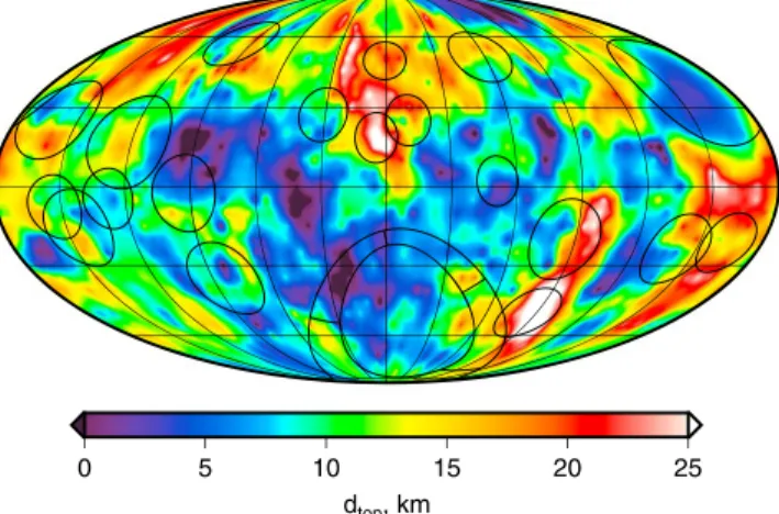
The second possibility for the origin of the magnetic carriers is that they were delivered to the Moon during large impact events. For this scenario, one might expect that the magnetization would be shallowest within and surrounding the largest basins. The depth to the top of the magnetized region is replotted in Figure 9