Does Monetary Policy Respond to Commodity Price Shocks?

(1)

HAL Id: hal-01511915

https://hal.archives-ouvertes.fr/hal-01511915

Submitted on 21 Apr 2017

HAL is a multi-disciplinary open access archive for the deposit and dissemination of sci-entific research documents, whether they are pub-lished or not. The documents may come from teaching and research institutions in France or abroad, or from public or private research centers.

L’archive ouverte pluridisciplinaire HAL, est destinée au dépôt et à la diffusion de documents scientifiques de niveau recherche, publiés ou non, émanant des établissements d’enseignement et de recherche français ou étrangers, des laboratoires publics ou privés.

Does Monetary Policy Respond to Commodity Price

Shocks?

Kuhanathan Ano Sujithan, Sanvi Avouyi-Dovi, Lyes Koliai

To cite this version:

Kuhanathan Ano Sujithan, Sanvi Avouyi-Dovi, Lyes Koliai. Does Monetary Policy Respond to Com-modity Price Shocks?. 62nd annual meeting of the AFSE, Jun 2013, Marseille, France. pp.52. �hal-01511915�

(2)

1

Does Monetary Policy Respond to Commodity Price Shocks?

Kuhanathan ANO SUJITHAN

†

Sanvi AVOUYI-DOVI

*

Lyes KOLIAI

†

First Draft

Abstract

Commodity prices, especially oil prices, peaked in the aftermath of the financial crisis of 2007 and they have remained highly volatile. All things being equal, the increase in commodity prices may induce a similar tendency of inflation and hence become a monetary policy issue. However, the impact of the changes of commodity prices on inflation is not clear. In this paper, by using Markov-switching models we show that there is an implicit impact of commodity markets on short-term interest rates for a set of heterogeneous countries (the U.S., the Euro area, Brazil, India, Russia and South Africa) over the period from January 1999 to August 2012. Besides, the VAR models reveal that short-term interest rates respond to commodity volatility shocks whatever the country. Moreover, the linkage between commodity markets and monetary policy instruments is stronger since the recent financial crisis.

JEL Classification: E43, E52, E58

Keywords: Monetary Policy, Commodity prices, Markov-switching, VAR models

(†) Paris-Dauphine University

(*) Banque de France and Paris-Dauphine University. Corresponding author Tel.: +33142929084, e-mail address: sanvi.avouyi-dovi@banque-france.fr

(3)

2

Hamilton (1983), Gisser and Goodwin (1986) and Mork (1989), among others, analyzed the effects of oil price shocks on real activity after a decade characterized by low growth rates in developed economies, volatile inflation and two major oil crises (1973 and 1979). The main findings of this body of literature are: oil price shocks have both inflationary effects and negative impact on output. Besides, one strand of the literature examined the role of commodity prices in the conduct of monetary policy. Our paper is related to this latter in which the changes in commodity prices have assumed to be one of the relevant sources of information for the conduct of monetary policy. Following the work of Hall (1982) regarding the role of the commodity prices for the Fed monetary policy, many studies have been performed:

i) Garner (1985, 1989) argued that central bankers should not target commodity prices as they cannot control them. He showed that even though commodity prices can provide useful information, Consumer Price Index (CPI) and commodity prices are not fully cointegrated;

ii) According to Boughton and Branson (1988),commodity prices could be interpreted as a leading indicator of CPI, in other words, turning points in commodity prices frequently preceded turning points in CPI inflation;

iii) Furlong (1989) noticed that commodity prices can help improve inflation forecasting. As a consequence, they can be useful for the conduct of monetary policy;

iv) According to Cody and Mills (1991), taking into account commodity prices in the monetary policy decisions significantly impacts inflation and output dynamics. In addition, they stress that the Federal Reserve (Fed) made its policy decisions without using information from commodity prices.

More recent papers do not confirm this view. They reveal that the links between commodity prices and inflation are time-varying; as a result, they are not entirely appropriate for central bankers. For instance, according to Bloomberg and Harris (1995), commodity prices are reliable forecasters of CPI in the 1970s and early 1980s but not in the mid 1980s. This result could be explained by the declining share of commodities in the US economy. Furlong and Ingenito (1996) obtained a similar conclusion. Polley and Iombra (1999) argued that commodity prices do not provide any significant information on the dynamics of interest rate spread and exchange rate. So, the role of commodity prices in the conduct of monetary policy is marginal since the 1990s, they have been omitted from analysis frameworks of monetary policy. However, Barsky and Kilian (2002), Frankel (2007), among others, studied the topic in another aspect, investigating the impact of monetary policy on commodity prices. Other strands of literature focused on the impact of commodity prices on expected inflation (Awokuse and Yang, 2003). Besides, according to Kilian and Lewis (2009), the traditional monetary policy framework should be replaced by a Dynamic Stochastic General Equilibrium (DSGE) model that takes into account the endogeneity of the oil price. The results of an estimated DSGE model performed by Bodinger et al. (2012) allow to confirm the proposals of Kilian and Lewis (2009). They concluded that central bankers should respond to oil price fluctuations.

Most of these studies focus on the US economy. Few papers regarding the others countries are available. Indeed, Boughton and Branson (1988) worked on a sample of developed countries; the paper by Hamori (2007) is devoted to the Japanese economy; Bloch et al. (2006) analyzed two major commodity exporters – Australia and Canada; Ocran and Biepke (2007) investigated the case of South Africa; the paper by Hassan and Salim (2011) is devoted to Australia.

(4)

3

Our paper aims to study the relationship between commodity prices and the dynamics of monetary policy instruments. We consider a set of heterogeneous countries (the US, the Euro area, Brazil, India, Russia and South Africa). The analysis is performed over the period span from January 1999 to August 2012. We model commodity prices using EGARCH-M models in order to highlight some stylized facts regarding the volatility of these prices. The aim of this point is to compare this volatility to the dynamics of monetary policy instruments. Then, we examine the links between monetary policy instruments and the fluctuations of commodity prices. More precisely, we look for the co-movement between the commodity prices cycles and that of the instruments of monetary policy. To do so, assuming that monetary policy instrument is short-term interest rates, we estimate for this instrument AR(p)-Markov-switching models with Time-Varying Transition Probabilities (TVTP) governed by commodities prices. Then, we implement VAR models, widely used in this body of literature, and study impulse responses to commodity price shocks, with unrestricted models and a baseline restricted model suitable for all countries. Finally, we study threshold VAR models.

The remainder of the paper is organized as follows. Section I provides a general overview based on a brief description of both the monetary policy frameworks of the previously mentioned six countries and the stance of commodities in these economies. Section II describes the recent developments in commodity markets. Section III provides a presentation of the models and the empirical results including robustness checks analyses. Section IV concludes.

I. General overview

If commodity prices are introduced in the decision making procedures of central banks, it should exist significant links between these prices and monetary policy instruments. Statuses and institutional objectives of central banks determine their monetary policy frameworks. Due to the heterogeneity of the set of countries under review in this paper, it is worth noting to examine the different frameworks in order to identify and establish their key factors.

Regarding the Fed, the main objectives are to stabilize inflation (currently a target of 2%) and to act in favor of full employment. These objectives lead to insure stability of long term interest rates. In order to comply with these objectives, Fed can adjust the Fed Funds rate; during the recent financial crisis, some unconventional measures, like Quantitative Easing (QE) programs, have been set up in order to provide markets with liquidity. The European Central Bank (ECB) has a single objective: to stabilize inflation (currently a target of 2%). Its main instruments are the refinancing Refi. (MRO, etc.) rates. The ECB also implemented some unconventional measures (the Securities Market Program) for the similar reasons. Brazil and South Africa display inflation targeting policies:

- The Central Bank of Brazil (CBB) has a CPI inflation target of 4.5% with a tolerance of 2 points. The main tool at CBB’s disposal is the SELIC rate on overnight collateralized loans; - The South African Reserve Bank (SARB) has a CPI inflation target range from 3 to 6%. Its key

policy rate is the Repurchase rate.

The Reserve Bank of India (RBI) adopted the multiple instruments approach. Its objectives are to maintain price and financial stability on one hand, to ensure sufficient flow of credit to productive sectors on the other hand. To comply with its objectives, RBI uses two key rates: the repo and the reverse repo rates. In addition, RBI also uses different reserve requirements: Cash reserve ratio (CRR) and Statutory liquidity ratio (SLR). Finally, The Bank of Russia (BoR) has a double target: an

(5)

4

inflation target and an exchange rate target. To achieve both targets BoR can adjust reserve requirements or act directly on financial markets via the open market operations (OMOs).

To sum up, these central banks have CPI inflation as one of their main target. The control of short-term interest rates as a monetary policy instrument is another common characteristic of these banks.

Regarding the commodities, in a more general perspective, they can induce some differences between countries under review: the sample includes three net commodity exporters (Russia, Brazil and South Africa) and three net commodity importers (the U.S., the Euro area and India). In 2011, India displays one of the highest negative commodity trade balances (-7.2% of GDP versus -2.1% for the U.S., see Table 1). The ratio of commodity exports to GDP of India is also relatively high (around 8% of GDP). The net exporters group is also heterogeneous: commodity trade balance to GDP is 15% in Russia, three times as high as that of Brazil. The ratio of commodity exports to GDP of Russia is really impressive (around 18%).

To be more precise, (see Table 2) Brazil is a net exporter of crude oil but a net importer of processed oil; India is in a symmetric position. The Euro area, the US and South Africa are net importers of energy (oil and gas). As a consequence, commodity prices swings will differently affect these countries. For illustration purposes, an increase in commodity prices, will boost export revenues, stimulate aggregate demand and will, most likely, lead the economy to inflationary pressures through demand in the case of Russia, for India or the US, inflationary pressures will be driven only by supply side.

Table 1 - Commodity trade to GDP ratios (in %)

U.S.A Euro area Brazil India Russia South Africa

Commodity exports to GDP 2.48 2.36 6.55 7.94 17.55 13.60 Commodity trade balance to GDP -2.11 -3.62 4.10 -7.23 14.99 6.25

(6)

5 Table 2 – Trade profiles for major commodities

Developed Economies Emerging Economies

U.S.A. Euro area Brazil Russia India S.A

Crude oil

-

+

-

Oil, not crude

-

+

-

Gas

-

+

-

Gold

+

N/A

-

+

Copper

-

+

Wheat

+

-

+

-

Soybeans

+

-

+

-

+

Corn

+

-

+

Coffee

-

+

-

+

-

Sugar

-

+

-

+

+ Net exporter / - Net importer; N/A: non available

Sources: International Trade Center (ITC) database and authors’ calculations, 2011

II. Recent developments in commodity markets

II.1 Which commodity prices and instruments of monetary policy to use?

Empirical evidence can be sensitive to the choice of commodity prices or instruments of monetary policy on one hand, to the sample period under review or data frequency on the other hand. As a consequence, the selection of the indicators and the sample period should be made carefully. The dataset is drawn from Datastream. Database covers six countries (the US, the Euro area, Brazil, India, Russia and South Africa). China is omitted from our analysis since its financial markets is less liberal compared with those of the countries under review.

Database consists of monthly observations from January 1999 to August 2012. 1 This frequency is more appropriate to describe the stance of monetary policy. In addition, it enables us to introduce macroeconomic factors in our framework. Besides, the starting date was selected for consistency reasons: the single monetary policy is conducted in the Euro area since 1999. The period under review contains many cycles (episodes of expansions and recessions) of commodity prices as well as phases of conventional and unconventional monetary measures. So, it seems convenient to analyze the links between commodity prices and monetary policy over this specific period.

1

(7)

6

The first differences of the variables or of the logarithm of the variables are stationary series (see Appendix 2).

Here, we employ two commodity price indicators: i) the Commodity Research Bureau (CRB) index, which is a composite index that includes a large set of commodities, and (ii) the Brent, as crude oil price. It is one of the most important and scrutinized commodity prices.

We also consider the underlying volatilities evaluated by the EGARCH-M models that we estimated in the following subsection. Our final monetary target is measured by the CPI. 2 Short-term interest rate (domestic interbank 3-month interest rate) acts as an indicator of monetary policy. We assume that the short-term rate is the most appropriate instrument as it reflects the stance of monetary policy and is highly sensitive to market changes.

Overall, our series show a mean close to zero. Broadly, short-term interest rates decreased over the period. Most of the series are leptokurtic and show negative skewness. The standard deviations of short-term interest rates are rather high for Russia and Brazil over the period, reflecting their domestic financial issues (banking crisis for Russia, debt crisis for Brazil).

II.2. Some observations on commodity prices and instruments of monetary policy

Between 1999 and 2002, non-fuel commodities prices declined steadily while oil prices were fairly stable. After that period, all commodity prices rose sharply from 2003 (see Figure 1). The amplitude of the rise was large and unprecedented. In addition, this trend was displayed by some major commodities: metals, minerals and oil. The price of the barrel of crude oil was around $25 in 2002; it reached $140 six years later (summer 2008). Although food commodity prices rose, it was nothing comparable with metals, minerals and oil. If we look at prices in real terms, only this last group of commodities reached all-time high prices.3 In addition, prices continued to rise even after the occurrence of the subprime crisis in 2007. Prices peaked during the summer 2008 and then fell sharply to reach the levels of 2005 at the beginning of 2009. Various factors linked to both demand and supply sides explain the fluctuations of these prices. Increasing demand was due to a combination of sources: (i) strong growth of major emerging economies such as China and India, (ii) the weakness of dollar, (iii) the growing demand for bio fuels which increased demand for agricultural commodities, and (iv) the “financialization” of commodity markets and as a consequence, a sharp development of speculation on these markets. On the supply side, it is a common knowledge that the increase in demand was unexpected thus leading to shortfalls. Regarding oil, we can also stress that shortfalls were associated with geopolitical unrest and uncertainty (Iraq, Iran, etc.). The collapse of commodity prices after mid-2008 is mainly explained by the global economic crisis with lower growth rates and rather negative expectations related to the uncertainty regarding the global real activity.

2

Activity indicators such as industrial production index, retail sale index or confidence index are not available for some countries of our panel in monthly frequency. As a consequence, we do not introduce monthly real activity indicators in the empirical analysis.

3

Recent commodity market developments: trends and challenges, United Nations Conference on Trade and

(8)

7 Figure 1 – Commodity prices

Sources: Datastream and authors’ calculations

However, commodity prices were back to an increasing trend starting mid-2009. The fast recovery in emerging economies explains such a phenomenon; the global crisis seemed only to have slowed down their growth. Emerging economies are still pulling the global demand for commodities. According to Radetzki (2006), their demand is driven by long term and structural factors which have positive outlooks. On the supply side, 2010 has been marked by shortfalls, especially in agricultural commodities following droughts in Eastern Europe and Russia and flood in Asia.

Even though prices remain quite high and rather volatile, the peak of 2008 has not been reached anymore. In order to improve our understanding of the dynamics of commodity prices, it is interesting to model and to jointly estimate the changes of these prices and their volatility. To do so, we propose to study both the log variations of the Brent (or log variations of the CRB) and its volatility using an EGARCH-M model.4

For the commodity return process{𝑦_𝑡}_𝑡=1𝑇 , an EGARCH-M(p,q) model is defined by

𝑦

𝑡

= 𝜇 + 𝛿ℎ

𝑡

+ 𝑧

𝑡

�ℎ

𝑡

log(ℎ

𝑡

) = 𝛼

0

+ � 𝛼

𝑖

𝑧

𝑡−𝑖 𝑞 𝑖=1

+ � 𝛾

𝑖

(|𝑧

𝑡−𝑖

| − 𝔼|𝑧

𝑡−𝑖

|)

𝑞 𝑖=1

+ � 𝛽

𝑖

log(ℎ

𝑡−𝑖

)

𝑝 𝑖=1

𝑧

𝑡

~i. i. d. (0,1)

where 𝛽_𝑖captures the GARCH dynamic of the conditional variance; 𝛼_𝑖the ARCH effects and 𝛾_𝑖the leveraged asymmetry effects on the conditional variance,

𝛿

represents the ARCH-in-mean effect. Using standard information criteria, we retained an M (2,1) for the Brent and an EGARCH-M(2,2) for the CRB. Most estimated parameters are significant (see Appendix 3) for the two indices. Both commodity prices are impacted negatively by their volatility ( 𝛿̂ being negative in both models).

4_{The results of our estimations will be used later on.}

100 150 200 250 300 350 400 450 500 550 600 100 300 500 700 900 1 100 1 300 1 500

Price of Brent and CRB Index (Jan. 1999=100)

Brent (left scale) CRB Index (right scale)

June 2008, average Barrel of brent = $132

(9)

8

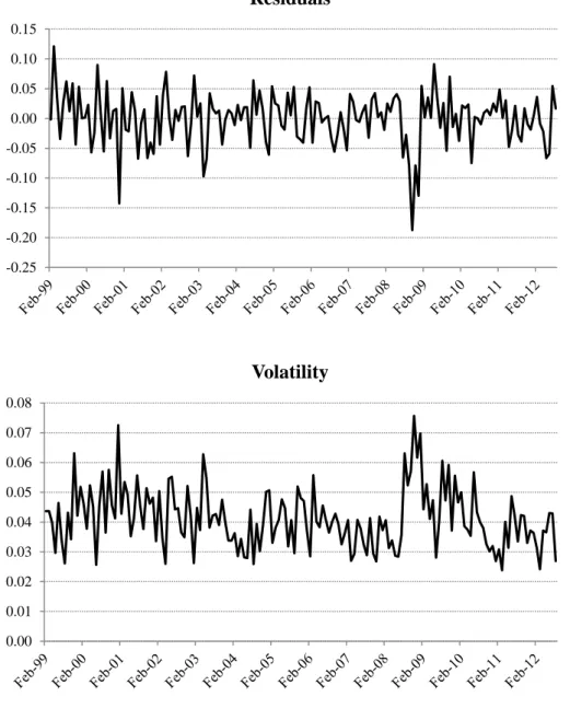
Moreover, CRB experiences a greater impact from its volatility than the Brent. In addition, volatility has been higher since 2008 for both series, and especially for the CRB (see Figures 2 and 3).

Figure 2 – Estimated residuals and volatility for the Brent from an EGARCH-M(2,1) model

-0.25 -0.20 -0.15 -0.10 -0.05 0.00 0.05 0.10 0.15

Residuals

0.00 0.01 0.02 0.03 0.04 0.05 0.06 0.07 0.08

Volatility

(10)

9

Figure 3 – Estimated residuals and volatility for the CRB from an EGARCH-M(2,2) model

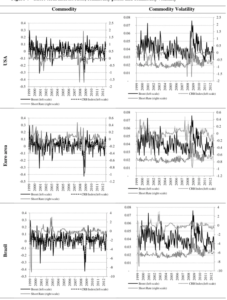
For the six countries, we observe that short rates dynamics and commodity prices show similar patterns (see Figure 4). While comparing short rates with commodity volatility, we note that short rates move oppositely to volatility, with the exception of Russia, which show similar patterns for both (see Figure 4). This phenomenon is especially noticeable with CRB’s volatility during the recent high volatility episodes. -0.10 -0.08 -0.06 -0.04 -0.02 0.00 0.02 0.04 0.06 0.08

Residuals

0.00 0.01 0.01 0.02 0.02 0.03 0.03 0.04 0.04 0.05 0.05

Volatility

(11)

10

Figure 4 – Short-term interest rates, commodity prices and commodity volatility

Commodity Commodity Volatility

US A E u ro a rea B ra zi l -2 -1.5 -1 -0.5 0 0.5 1 1.5 2 2.5 -0.5 -0.4 -0.3 -0.2 -0.1 0 0.1 0.2 0.3 0.4 1 9 9 9 2 0 0 0 2 0 0 1 2 0 0 2 2 0 0 3 2 0 0 4 2 0 0 5 2 0 0 6 2 0 0 7 2 0 0 8 2 0 0 9 2 0 1 0 2 0 1 1 2 0 1 2

Brent (left scale) CRB Index(left scale)

Short Rate (right scale)

-2 -1.5 -1 -0.5 0 0.5 1 1.5 2 2.5 -0.01 0.02 0.03 0.04 0.05 0.06 0.07 0.08 1 9 9 9 2 0 0 0 2 0 0 1 2 0 0 2 2 0 0 3 2 0 0 4 2 0 0 5 2 0 0 6 2 0 0 7 2 0 0 8 2 0 0 9 2 0 1 0 2 0 1 1 2 0 1 2

-1.2 -1 -0.8 -0.6 -0.4 -0.2 0 0.2 0.4 0.6 -0.5 -0.4 -0.3 -0.2 -0.1 0 0.1 0.2 0.3 0.4 1 9 9 9 2 0 0 0 2 0 0 1 2 0 0 2 2 0 0 3 2 0 0 4 2 0 0 5 2 0 0 6 2 0 0 7 2 0 0 8 2 0 0 9 2 0 1 0 2 0 1 1 2 0 1 2

-1.2 -1 -0.8 -0.6 -0.4 -0.2 0 0.2 0.4 0.6 -0.01 0.02 0.03 0.04 0.05 0.06 0.07 0.08 1 9 9 9 2 0 0 0 2 0 0 1 2 0 0 2 2 0 0 3 2 0 0 4 2 0 0 5 2 0 0 6 2 0 0 7 2 0 0 8 2 0 0 9 2 0 1 0 2 0 1 1 2 0 1 2

-10 -8 -6 -4 -2 0 2 4 -0.5 -0.4 -0.3 -0.2 -0.1 0 0.1 0.2 0.3 0.4 1 9 9 9 2 0 0 0 2 0 0 1 2 0 0 2 2 0 0 3 2 0 0 4 2 0 0 5 2 0 0 6 2 0 0 7 2 0 0 8 2 0 0 9 2 0 1 0 2 0 1 1 2 0 1 2

-10 -8 -6 -4 -2 0 2 4 -0.01 0.02 0.03 0.04 0.05 0.06 0.07 0.08 1 9 9 9 2 0 0 0 2 0 0 1 2 0 0 2 2 0 0 3 2 0 0 4 2 0 0 5 2 0 0 6 2 0 0 7 2 0 0 8 2 0 0 9 2 0 1 0 2 0 1 1 2 0 1 2

(12)

11

Commodity Commodity Volatility

India Ru ssi a So ut h A fr ic a

Sources: Datastream and authors’ calculations

-2.5 -2 -1.5 -1 -0.5 0 0.5 1 1.5 2 -0.5 -0.4 -0.3 -0.2 -0.1 0 0.1 0.2 0.3 0.4 1 9 9 9 2 0 0 0 2 0 0 1 2 0 0 2 2 0 0 3 2 0 0 4 2 0 0 5 2 0 0 6 2 0 0 7 2 0 0 8 2 0 0 9 2 0 1 0 2 0 1 1 2 0 1 2

-2.5 -2 -1.5 -1 -0.5 0 0.5 1 1.5 2 -0.01 0.02 0.03 0.04 0.05 0.06 0.07 0.08 1 9 9 9 2 0 0 0 2 0 0 1 2 0 0 2 2 0 0 3 2 0 0 4 2 0 0 5 2 0 0 6 2 0 0 7 2 0 0 8 2 0 0 9 2 0 1 0 2 0 1 1 2 0 1 2

-50 -40 -30 -20 -10 0 10 -0.5 -0.4 -0.3 -0.2 -0.1 0 0.1 0.2 0.3 0.4 1 9 9 9 2 0 0 0 2 0 0 1 2 0 0 2 2 0 0 3 2 0 0 4 2 0 0 5 2 0 0 6 2 0 0 7 2 0 0 8 2 0 0 9 2 0 1 0 2 0 1 1 2 0 1 2

-50 -40 -30 -20 -10 0 10 -0.01 0.02 0.03 0.04 0.05 0.06 0.07 0.08 1 9 9 9 2 0 0 0 2 0 0 1 2 0 0 2 2 0 0 3 2 0 0 4 2 0 0 5 2 0 0 6 2 0 0 7 2 0 0 8 2 0 0 9 2 0 1 0 2 0 1 1 2 0 1 2

-1.5 -1 -0.5 0 0.5 1 1.5 -0.5 -0.4 -0.3 -0.2 -0.1 0 0.1 0.2 0.3 0.4 1 9 9 9 2 0 0 0 2 0 0 1 2 0 0 2 2 0 0 3 2 0 0 4 2 0 0 5 2 0 0 6 2 0 0 7 2 0 0 8 2 0 0 9 2 0 1 0 2 0 1 1 2 0 1 2

-1.5 -1 -0.5 0 0.5 1 1.5 -0.01 0.02 0.03 0.04 0.05 0.06 0.07 0.08 1 9 9 9 2 0 0 0 2 0 0 1 2 0 0 2 2 0 0 3 2 0 0 4 2 0 0 5 2 0 0 6 2 0 0 7 2 0 0 8 2 0 0 9 2 0 1 0 2 0 1 1 2 0 1 2

(13)

12

In order to analyze the impact of the recent crisis on the dynamics of commodity prices and the short-term interest rates, we split the sample into two sub-periods: before (from January 1999 to August 2008) and after (from August 2008 to August 2012) the Lehman collapse. We calculate correlations between commodity prices and short rates in order to highlight the differences between the two sub-periods. The correlation between commodity prices and short rates was close to 0 for all economies before August 2008. Since then, it has become positive and significantly different from 0 for the US, the Euro area and India; which are net commodity importers. Conversely, correlation has become negative for net commodity exporters (Brazil, Russia and South Africa). The correlations between oil price volatility and short rates are, in general, different from 0 and higher after the Lehman Brothers collapse. The correlations between CRB volatility and short rates are close to zero before the collapse but they are, in general, significantly different from 0 after August 2008 with exception for Russia and Brazil.

Table 3 – Linear correlation between commodity prices and short rates

Sub-period USA EURO BRAZIL INDIA RUSSIA SA

Δl Brent Until August 2008 -0.07 -0.01 0.00 0.04 -0.04 0.05 After August 2008 0.27 0.30 -0.18 0.42 -0.44 -0.21

Δl CRB Until August 2008 0.08 -0.01 0.02 0.01 0.02 0.01

After August 2008 0.16 0.30 -0.01 0.40 -0.45 -0.06 Brent Volatility Until August 2008 -0.15 -0.08 0.08 -0.24 -0.02 -0.13 After August 2008 -0.27 -0.54 0.01 -0.34 0.35 -0.24 CRB Volatility Until August 2008 0.02 0.05 0.00 0.08 0.02 -0.01 After August 2008 -0.45 -0.51 0.01 -0.61 0.10 -0.22 Sources: Datastream and authors’ calculations. Δl X= ln (X/X-1)

III. Understanding evidence on the relationships between commodity prices

and instruments of monetary policy

III.1 Specification of Markov-Switching models

In order to identify the different phases in the dynamics of the variables (instruments of monetary policy, etc.), we specify and estimate Markov-switching models for the instruments of monetary policy. Indeed, Markov-switching models provide a simple way to disentangle the regimes affecting the fluctuations of these variables. More precisely, for each country, we model the dynamics of short-term interest rate via a Markov-switching process. According to Filardo (1994), we assume that the transition probabilities vary over time. So, we set up Markov-switching models combined with time-varying transition probabilities (MS-TVTP). We consider a two regime process. Each regime is characterized by an AR(p) process. The transition probabilities depend on a commodity prices –CRB or Brent- and / or their volatilities.

(14)

13 Δ𝑦𝑡 = 𝜇𝑆𝑡+ � 𝜓𝑆𝑡,𝑖Δ𝑦𝑡−𝑖+ 𝑘 𝑖=1 𝜎𝑆𝑡𝜀𝑡, where, 𝜇_𝑆_𝑡= 𝜇₀+ 𝑆_𝑡(𝜇₁− 𝜇₀),𝜓_𝑆_𝑡,𝑖 = 𝜓_0,𝑖+ 𝑆_𝑡�𝜓_1,𝑖− 𝜓_0,𝑖�, 𝜎_𝑆_𝑡= 𝜎_0,𝑖+ 𝑆_𝑡(𝜎₁− 𝜎₀), 𝜀_𝑡~𝒩(0,1), 𝑘 is the lag order and 𝑆𝑡 ∈ {1,2}.

The Ar(p) process and the innovation are state-dependant with respect to a state variable 𝑆_𝑡. This state variable{ 𝑆_𝑡}_𝑡=1𝑇 follows a first-order two-state Markov process with a time-varying transition matrix𝑃_𝑡 defined by 𝑃(𝑆𝑡 = 𝑠𝑡|𝑆𝑡−1= 𝑠𝑡−1, 𝑧𝑡) = � 𝑝_{1 − 𝑝}11(𝑧𝑡) 1 − 𝑝22(𝑧𝑡) 11(𝑧𝑡) 𝑝22(𝑧𝑡) �, where, 0 ≤ 𝑝𝑖𝑗,𝑡≤ 1, � 𝑝𝑖𝑗,𝑡 = 1 2 𝑖=1 𝑎𝑛𝑑 𝑗 = 1,2 𝑝11,𝑡(𝑧𝑡) = 𝑃(𝑆𝑡 = 1|𝑆𝑡−1= 1, 𝑧𝑡) = Φ(𝛼1+𝛽1𝑧𝑡) 𝑝22,𝑡(𝑧𝑡) = 𝑃(𝑆𝑡 = 2|𝑆𝑡−1 = 2, 𝑧𝑡) = Φ(𝛼2+𝛽2𝑧𝑡)

The matrix components are estimated each date 𝑡 using a univariate probit model (Krolzig, 1997) as the functional form of the probabilities.5

𝑧𝑡 is the vector of exogenous variables that governs the dynamics of the transition probabilities and

𝛽𝑖(𝑖 = 1,2) are the parameters associated with 𝑧𝑡 in each regime. Models are estimated using the

maximum likelihood method.

Models using the CRB as exogenous variable of transition probabilities performed poorly for the US and was a little less accurate for the Euro short rate. Likewise, models using the Brent as 𝑧_𝑡 were not properly fitted for India and Russia. In the case of Brazil and South Africa, they were quite similar but we decided to include the models with the CRB and group them with the emerging economies (see Appendix 4). As a consequence, we have set 𝑧_𝑡 to be the Brent (respectively CRB) for the US and the Euro area (respectively for Brazil, India, Russia and South Africa).

As expected, the models detect two distinct regimes and the main coefficients are significantly different from zero for each country (see Tables 4). The models outline only few ‘”high volatility” periods for the US, the Euro area and Brazil whereas there are long periods of “high volatility” regime for Russia and many shifts in the case of India and South Africa (see Appendixes 5 and 6). We can stress the link between the “high volatility” regime in the dynamics of short rates with episodes of expansions and recessions of the commodity prices. Symmetrically, less turbulent episodes in commodity markets seem to draw short rate dynamics towards a “low volatility” regime (see Appendixes 5 and 6).

5

The logistic functional form could also be used for defining the transition probability (see Filardo, 1994).

(15)

14

On a country level, the regimes identified by the models (i.e. the link between commodity returns and a monetary policy instrument) differ in many regards. The duration of “low volatility” regimes identified by the models are more important for all countries except South Africa. Both regimes have equivalent durations for South Africa, while showing high durations in both regimes for Russia.

Table 4a –MS-TVTP for the US with Brent

Constant Sigma α β Duration (months) Log Likelihood State 1 0.03* 0.01* 1.95* -1.08* 25 54.85 (0.01) (0) (0.33) (0.35) State 2 -0.27** 0.4* 5.57** 0.8 7 (0.14) (0.07) (2.29) (4.28)

Table 4b –MS-TVTP for the Euro area with Brent

Constant Sigma α β Duration (months) Log Likelihood State 1 0.01 0.02* 3.17* -0.41 59 80.1 (0.01) (0) (1.61) (0.69) State 2 -0.62* 0.07 10.07 1.93 3 (0.14) (0.12) (11.64) (7.75)

Table 4c –MS-TVTP for Brazil with CRB

Constant Sigma α β Duration (months) Log Likelihood State 1 -0.07*** 0.18* 2.03* -1.12 47 -140.5 (0.04) (0.02) (0.29) (1.12) State 2 -1.33 9.87** 0.04 9.8 6 (1.12) (3.86) (12.7) (17.22)

Table 4d –MS-TVTP for India with CRB

Constant Sigma α β Duration (months) Log Likelihood State 1 0.07* 0.04* 1.03* -0.67 7 -76.87 (0.02) (0.01) (0.25) (0.44) State 2 -0.15 0.56* -0.79 13.18 3 (0.12) (0.13) (5.58) (10.35)

(16)

15 Table 4e –MS-TVTP for Russia with CRB

Constant Sigma α β Duration (months) Log Likelihood State 1 -0.07* 0.55* 6.62* -1.84* 5e10 -305.19 (0) (0) (0) (0) State 2 -0.54* 15.61* 0.04* -5.03* 28 (0) (0) (0) (0)

Table 4f –MS-TVTP for South Africa with CRB

Constant Sigma α β Duration (months) Log Likelihood State 1 0 0.004* 0.45** -0.51** 3 -18.66 (0.01) (0) (0.2) (0.21) State 2 -0.12* 0.26* 4.28 -7.42 3 (0.06) (0.04) (3.81) (4.65)

Standard errors are in parenthesis. *, ** and *** denote respectively 1%, 5% and 10% significance To sum up, due to parameter estimates significance, we need to consider the presence – at some extent – of an implicit impact of commodity markets on short rate series.

In order to check the robustness of the results drawn from the univariate models, we compare them to a benchmark linear model. Then, we estimate a series of less flexible Markov-switching models in which variances are not state dependent (

𝜎

₁

= 𝜎

₂

)

. We report standard statistics such as AIC, LR and we calculate regime classification measures (RCM, see Ang and Bekaert, 2002).6 The regime classification measure is given by:

𝑅𝐶𝑀 = 400 ×1_{𝑇 � 𝑝}11,𝑡(1 − 𝑝11,𝑡) 𝑇

𝑡=1

RCM are better for Markov-switching models but the models with fixed variance dominate the others. Overall, within the framework of fixed variance, models show better LR tests (see Table 5). Nevertheless, we observe that these models show very few significant parameters (see Appendix 7); the results of RCM could be explained only by the dynamic properties of the variables. Moreover, there is no economic motivation or intuition that would back the hypothesis of fixed variance. Hence, we prefer our set of models which seems more consistent with economic intuition.

6

The RCM is a summary point statistic which describes the quality of regime classifications. Good regime classification is associated with low RCM values. If the RCM is close to zero, the regime classification is perfect whereas a value of 100 means that no information about regimes is revealed.

(17)

16 Table 5 – Identification procedure

USA Euro Brazil India Russia

South Africa RCM Linear regression 100 100 100 100 100 100 MS-TVTP 8.94 2.09 6.00 38.81 3.60 30.18 MS-TVTP with σ1=σ2 0.78 0.06 0.00 2.59 0.19 2.78 LR test MS-TVTP -0.84 0.47 1.79 1.45 1.49 4.02 MS-TVTP with σ1=σ2 3.62 0.47 1.50 1.17 1.34 1.83

In order to test the relevance of Markov-switching specification for short rates and commodity prices dynamics, we perform the Markov-Switching Augmented Dickey–Fuller (MS-ADF) test proposed by Hall et al. (1999) 7 in order to detect explosive bubble behaviors in short-rate series.

Given the MS-ADF model specified as

Δ𝑦𝑡 = 𝜇𝑆𝑡+ 𝜙𝑆𝑡𝑦𝑡−1+ � 𝜓𝑆𝑡,𝑖Δ𝑦𝑡−𝑖+

𝑘 𝑖=1

𝜎𝑆𝑡𝜀𝑡,

where, 𝜙_𝑆_𝑡= 𝜙₀+ 𝑆_𝑡(𝜙₁− 𝜙₀) is the ADF coefficient. If we refer to the regime with a larger (resp. lower) ADF coefficient as regime 1 (resp. 0), the MS-ADF bubble test is defined as follows:

- In regime 1, the unit root null hypothesis is 𝜅₁≡ max(𝜙₀, 𝜙₁) = 0 against the explosive alternative 𝜅₁> 0.

- In regime 0, the unit root null hypothesis is 𝜅₀≡ min(𝜙₀, 𝜙₁) = 0 against the stationary alternative 𝜅₀ < 0.

We use parametric bootstrapping to obtain the critical values of the MSADF test, as in van Norden and Vigfusson (1998) and Shi (2012). 4000 replications are used in the bootstrapping, with model estimation coefficients as priors.

We reject the unit root null hypothesis of 𝜅₁ for Brent and CRB series at 10% and 1% significance levels respectively and we fail to reject that for short rate series at 10% confidence level (see Table 6). Furthermore, we fail to reject the unit root null hypothesis in regime 0 of all series at the 10% significance level. In other words, both Brent and CRB are mixtures of a unit root process and an explosive process, whereas short rate series seem to be driven by random walk processes.

7

Although this test was designed for Markov-switching models with fixed transition probabilities (FTP), we use it in our time-varying transition probabilities (TVTP) framework, since no adapted tests exists in the literature in such a framework. Additional study on the unit-root tests for MS-TVTP models would be an interesting research topic.

(18)

17 Table 6 – MS-ADF tests

Brazil India Euro USA Brent CRB

𝜅₀ 𝜅₁ 𝜅₀ 𝜅₁ 𝜅₀ 𝜅₁ 𝜅₀ 𝜅₁ 𝜅₀ 𝜅₁ 𝜅₀ 𝜅₁ Estimates Coefficients -0.653 -0.003 -0.082 0.521 0.016 0.228 -0.019 -0.002 -0.180 0.385 -0.113 0.546 ADF Stats -0.011 -0.329 -1.440 0.092 0.654 0.028 -1.814 -31.097 -2.740 0.083 -3.889 3.148 Critical Values 10% -2.40 0.60 -3.33 0.80 -2.34 66.46 -37.81 1.09 -101.84 -0.42 -88.79 -25.36 5% -2.90 0.90 -3.80 1.04 -3.43 70.25 -39.93 1.36 -125.81 0.01 -102.54 -0.13 1% -3.78 1.80 -4.46 1.54 -8.23 75.73 -44.11 2.10 -201.06 0.67 -128.94 0.60

Source: authors’ calculations

Since we find that univariate non-linear specification may be unsuited to model short rate and commodity prices, we propose to investigate a multivariate framework which allows a joint dynamic of these series.

III.2 What can we draw from a multivariate framework?

In order to analyze the joint relations between commodity prices and monetary policy instruments we estimate a basic VAR (p) (Sims, 1980). The VAR model includes the short-term interest rate, the CPI and the CRB volatility as estimated with EGARCH-M specifications in the previous section. Conventional information criteria (Akaike, Hannan-Quinn, etc.) help to evaluate p, the number of lags which turns to be 3. p=3, or one quarter in the context of monthly data, appears sufficient to take into account interactions between the variables. If 𝑦_𝑡 represents the vector of the variables, the model is given by

A(L)𝑦𝑡 = 𝑐 + εt

where A(L)is a polynomial matrix of degree p in the lag operator L, ε_t~𝒩₃(I₃, Σ) and 𝒩₃(∙) is the 3 −dimensional normal distribution. Estimates are realized using the OLS per equation method. To obtain the best empirical results, the estimation is performed in two steps:

- First, we estimated an unrestricted VAR(3) model for each economy;

- Second, in order to capture a common specification for the whole sample, we estimated a restricted VAR model that fits properly with significant parameters within the six considered economies.

Finally, we perform impulse responses for each estimated model in the case of a unit shock on the commodity variable.

We focus the analysis on the equations of short-term interest rates and especially on the value and significance of the coefficient of the commodity volatility in these equations.

In the set of unrestricted VAR(3), we observe that the commodity volatility impacts the short rate at some point (see Appendix 8). In all countries, with the exception of the Euro area, the short rate is impacted after a quarter by the CRB’s volatility. Brazil’s short rate is impacted negatively after a quarter, but the coefficient in absolute terms is significantly lower than one for the U.S. For the Euro

(19)

18

area and India, the short-term interest rate is impacted by the CRB volatility with a two-month delay. The coefficient is much higher though for India. For South Africa, the short rate is impacted negatively after a two-month delay but the impact is low and then we observe a positive impact after a quarter. In the case of Russia and the U.S, the equation of the short rate is impacted in opposite direction by the CRB volatility in lag one (positive coefficient) and three (negative coefficient).The absolute values of coefficients are close; nevertheless they are slightly superior for the first lag. With exception of Russia and the US, we can state at this point that higher commodity volatility induces lower short-term interest rates. In other words, the central banks reactions seem to be moderate when the commodity prices become volatile i.e. if uncertainty regarding commodity prices increases the central banks reactions are attenuated. These results are in line with those regarding central banks reactions when data uncertainty prevails.

In the restricted framework, which turns out to be a VAR (1), with the exception of India and the Euro area, all countries display a significant coefficient for the commodity volatility in their short rate equation (see Appendix 9). We have seen in the earlier model that the short rate for both the Euro area and India were impacted by commodity volatility first after two months. That might explain why we do not observe any significant impact in a specification restricted to one lag. Russia’s short rate increases with commodity volatility whereas in the other economies, the relation between short rate and commodity volatility is a decreasing one. The U.S. short rate is the one least impacted (coefficient of -2.1) while the short rates of Brazil and Russia are the most sensitive (respectively -8.2 and 26.7). However, the degree of the sensitivity of Brazil and Russia’s short-term rates to the commodity volatility is surprising and difficult to justify.

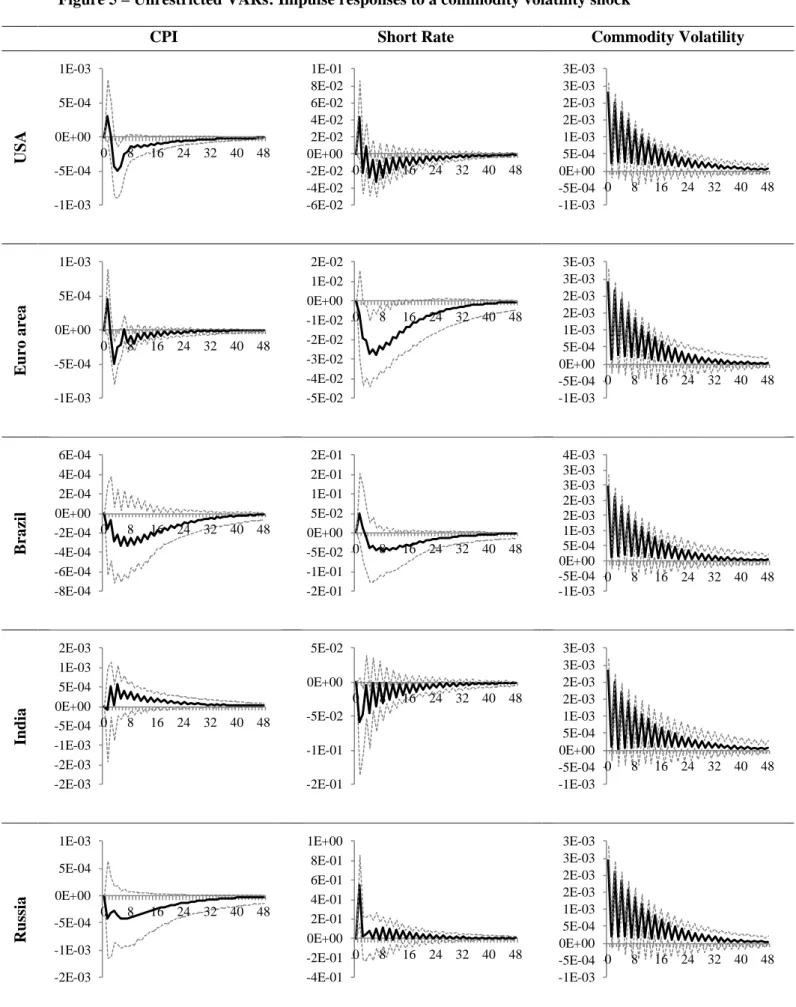
The impulse responses of the short-term rate for a commodity volatility shock lead to:

- The U.S. short rate increases in a first time before starting to decrease after one month (see Figure 5). It reaches its lowest values at around the second quarter after the initial shock;

- South Africa’s short rate is hit rapidly and peaks down after a quarter before starting its recovery; - The pattern which prevails for India is quite similar to South Africa’s response;

- The case of Russia is quite unique as it is the only economy in which the short rate increases after a shock. This might be explained by the large value of the coefficient of the commodity variable at the first lag in the short rate equation. The short rate peaks after a quarter and then decreases;

- Overall, the shock is absorbed rapidly, except for the Euro area and Brazil who experience a prolonged effect.

(20)

19

Figure 5 – Unrestricted VARs: Impulse responses to a commodity volatility shock

CPI Short Rate Commodity Volatility

US A E u ro a rea B ra zi l India Ru ssi a -1E-03 -5E-04 0E+00 5E-04 1E-03 0 8 16 24 32 40 48 -6E-02 -4E-02 -2E-02 0E+00 2E-02 4E-02 6E-02 8E-02 1E-01 0 8 16 24 32 40 48 -1E-03 -5E-04 0E+00 5E-04 1E-03 2E-03 2E-03 3E-03 3E-03 0 8 16 24 32 40 48 -1E-03 -5E-04 0E+00 5E-04 1E-03 0 8 16 24 32 40 48 -5E-02 -4E-02 -3E-02 -2E-02 -1E-02 0E+00 1E-02 2E-02 0 8 16 24 32 40 48 -1E-03 -5E-04 0E+00 5E-04 1E-03 2E-03 2E-03 3E-03 3E-03 0 8 16 24 32 40 48 -8E-04 -6E-04 -4E-04 -2E-04 0E+00 2E-04 4E-04 6E-04 0 8 16 24 32 40 48 -2E-01 -1E-01 -5E-02 0E+00 5E-02 1E-01 2E-01 2E-01 0 8 16 24 32 40 48 -1E-03 -5E-04 0E+00 5E-04 1E-03 2E-03 2E-03 3E-03 3E-03 4E-03 0 8 16 24 32 40 48 -2E-03 -2E-03 -1E-03 -5E-04 0E+00 5E-04 1E-03 2E-03 0 8 16 24 32 40 48 -2E-01 -1E-01 -5E-02 0E+00 5E-02 0 8 16 24 32 40 48 -1E-03 -5E-04 0E+00 5E-04 1E-03 2E-03 2E-03 3E-03 3E-03 0 8 16 24 32 40 48 -2E-03 -1E-03 -5E-04 0E+00 5E-04 1E-03 0 8 16 24 32 40 48 -4E-01 -2E-01 0E+00 2E-01 4E-01 6E-01 8E-01 1E+00 0 8 16 24 32 40 48 -1E-03 -5E-04 0E+00 5E-04 1E-03 2E-03 2E-03 3E-03 3E-03 0 8 16 24 32 40 48

(21)

20

So ut h A fr ic a

It is worth noting that the results within the restricted framework confirm those of our previous estimates: except for Russia, all short rates experience a decrease (see Figure 6). However, we observe that after two quarters, the short rates converge to their initial values. India’s short rate peaks down after a quarter and returns rapidly as well towards its former value. In all other economies, short rates recover slower than in the unrestricted models. This can be explained by the fact that only one lag is included in this specification, thus making all shocks more persistent. Besides, short rates recover more rapidly in emerging economies than in developed economies. This is probably due to the fact that – except for Russia which is a unique case – coefficients of commodity volatility are higher for the U.S. and the Euro area.

Figure 6 – Restricted VARs: Impulse responses to a commodity volatilityshock

US A E u ro a rea -2E-03 -1E-03 -5E-04 0E+00 5E-04 1E-03 0 8 16 24 32 40 48 -1E-01 -8E-02 -6E-02 -4E-02 -2E-02 0E+00 2E-02 4E-02 6E-02 8E-02 0 8 16 24 32 40 48 -1E-03 -5E-04 0E+00 5E-04 1E-03 2E-03 2E-03 3E-03 3E-03 0 8 16 24 32 40 48 0E+00 1E-04 2E-04 3E-04 4E-04 5E-04 6E-04 7E-04 0 8 16 24 32 40 48 -3E-02 -2E-02 -1E-02 0E+00 1E-02 2E-02 0 8 16 24 32 40 48 0E+00 1E-03 2E-03 3E-03 4E-03 5E-03 6E-03 7E-03 0 8 16 24 32 40 48 0E+00 1E-04 2E-04 3E-04 4E-04 5E-04 6E-04 7E-04 0 8 16 24 32 40 48 -3E-02 -2E-02 -2E-02 -1E-02 -5E-03 0E+00 5E-03 1E-02 0 8 16 24 32 40 48 0E+00 1E-03 2E-03 3E-03 4E-03 5E-03 6E-03 7E-03 0 8 16 24 32 40 48

(22)

21

B ra zi l India Ru ssi a So ut h A fr ic a 0E+00 2E-04 4E-04 6E-04 8E-04 1E-03 1E-03 1E-03 0 8 16 24 32 40 48 -2E-01 -2E-01 -1E-01 -5E-02 0E+00 5E-02 0 8 16 24 32 40 48 0E+00 1E-03 2E-03 3E-03 4E-03 5E-03 6E-03 7E-03 8E-03 0 8 16 24 32 40 48 0E+00 5E-04 1E-03 2E-03 2E-03 0 8 16 24 32 40 48 -4E-02 -3E-02 -2E-02 -1E-02 0E+00 1E-02 2E-02 0 8 16 24 32 40 48 0E+00 1E-03 2E-03 3E-03 4E-03 5E-03 6E-03 7E-03 8E-03 0 8 16 24 32 40 48 0E+00 5E-04 1E-03 2E-03 2E-03 3E-03 0 8 16 24 32 40 48 -2E-01 -1E-01 0E+00 1E-01 2E-01 3E-01 4E-01 0 8 16 24 32 40 48 0E+00 1E-03 2E-03 3E-03 4E-03 5E-03 6E-03 7E-03 0 8 16 24 32 40 48 0E+00 2E-04 4E-04 6E-04 8E-04 1E-03 1E-03 1E-03 0 8 16 24 32 40 48 -6E-02 -5E-02 -4E-02 -3E-02 -2E-02 -1E-02 0E+00 1E-02 0 8 16 24 32 40 48 0E+00 1E-03 2E-03 3E-03 4E-03 5E-03 6E-03 7E-03 0 8 16 24 32 40 48

(23)

22

III.3 Multivariate framework: Threshold VAR models

In previous sections, we explored linear specifications through unrestricted VAR models. We also found that Markov-switching models may be unsuited for the purpose of our study. Policy makers may react to commodity price variations only if there is a significant rise or fall, hence it may be relevant to introduce less restricted non-linear models that take into account threshold effects.

For each economy, short rate and CPI variables are stored in the 2 × 1 vector 𝑦_𝑡. The bivariate system switches between two regimes (“high growth” and “low growth”) according to the position of a commodity price changes 𝑧_𝑡with respect to a threshold value 𝜆. The Threshold Vector Autoregressive (TVAR) model is then specified as follows

𝑦𝑡 = �𝐴 (1)_(𝐿)𝑦

𝑡−1+ εt if 𝑧𝑡−𝑘≤ 𝜆

𝐴(2)_(𝐿)𝑦

𝑡−1+ εt if 𝑧𝑡−𝑘> 𝜆

where, 𝐴(1)and 𝐴(2) are polynomial matrix in the lag operator, 𝑘 the parameter of delay, 𝜀_𝑡~𝒩_𝑑(𝐼_𝑑, Σ) and 𝒩_𝑑(∙) the 𝑑-dimensional normal distribution.

To estimate the TVAR parameters, we replicate the strategy applied to the VAR models estimations in the previous section by: (i) estimating an unrestricted TVAR(3) model for each economy, then (ii) estimating a restricted common TVAR(1) model.

For the estimated TVAR(3) models, we notice that, except for Russia, the threshold level is around 2.4% of commodity volatility (ranging from 1.9% for Brazil to 2.7% for the US). In the case of Russia, the threshold level is -4.0%. Besides from Brazil and Russia, in all countries there are more observations during the “low growth” regime (see Appendix 10). During the “low growth” regime we find that only lagged coefficients impacts the short rate for both the U.S. and the Euro area. Developing economies show significant coefficients for short rate, CPI, at different levels, and for the intercept (except in the case of India). In the “high growth” regime, first of all, we notice that coefficients are from the opposite sign or are much larger. The Euro area shows similar features as in the first regime: the short rate is only impacted by its lagged values (to a larger extent). In the case of the US, Brazil and South Africa, the short rate is influenced by both its lagged values and those of CPI, at different levels. The equations for India and Russia do not show any significant coefficient. For the TVAR(1) models, the threshold level is positive for all countries and ranging from 1.7% for India to 2.7% the Euro area (see Appendix 11). With the exception of Brazil and India, all countries show a superior number of observations during the “low growth” regime. During the “low growth” regime for all countries, the short rate is only impacted by its lagged value. Once again, during the “high growth” regime, India and Russia’s short rates do not reveal any significant coefficient. For the U.S., Brazil and South Africa, all parameters are significant. The Euro area’s short rate is only influenced by its lagged value. In this regime, all coefficients are either from the opposite sign or much larger.

(24)

23

III.4 Robustness check issues

We propose to test the VAR models against two different specifications. First, we introduce a fourth variable in the models, a monetary aggregate M2.8 Unfortunately, as we lack of data for Russia’s M2, we cannot include it in this series of tests. Secondly, we estimate the models until August 2008 - prior to the Lehman brothers’ collapse. Finally, we compare forecasted values of the short-term interest rates’ with the actual ones (from August 2008 to August 2012).

Consistently with our previous analysis, we will emphasis results concerning the equations defining the short-term interest rates. While including M2 in our unrestricted systems, we find that these results comply mostly with our previous ones, with the exception of Brazil for which the relation between the short rate and commodity volatility collapses (see Appendix 12).Nevertheless, there is a link between M2 and CRB volatility which might also indicate an impact of commodity volatility on monetary policy for Brazil. The impact of commodity volatility on short rate is almost identical for the other countries. Coefficients are of the same range. The estimation of restricted systems including M2 leads to: no significant coefficient for the commodity volatility variable in the equations of the short rate for the U.S, the Euro area and India (see Appendix 13); the coefficients for Brazil and South Africa are consistent with the previous ones (same sign and same range). Once again, when the link between the short rate and the CRB volatility disappears, we observe a significant coefficient for the commodity variable in the M2 equations, which is at least a variable of interest for central bankers.

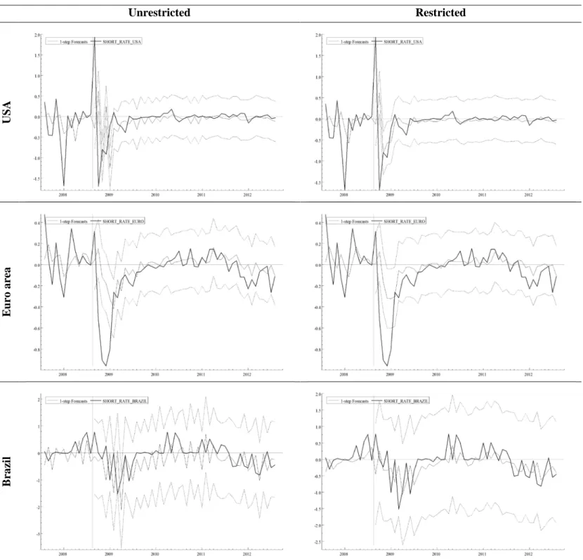
When estimating the models until August 2008, we observe that the relationship between commodity volatility and the short-term interest rates is very much different. First, let us have a look at the unrestricted systems. In the case of Russia, the significant coefficients appear to have the same sign but are much higher here (in absolute terms). The link between the variables of interest becomes insignificant for the U.S, the Euro area, India and South Africa (see Appendix 14).The short rate for Brazil is impacted earlier (at lag two) but the impact is much lower. For the restricted models estimated until August 2008, we note that there is no link between CRB volatility and short rate in the cases of the Euro area and India, which is consistent with our previous results; but also for Russia (see Appendix 15). For all the other economies, the results are consistent with the previous ones. Overall, we can explain these differences by arguing that the financial crisis modified the relation between commodity markets and monetary policy. Our results seem to confirm the idea that commodity markets are monitored more closely since the Lehman Brother’s collapse.

Using these two sets of models, we make recursive 1-step forecasts over the period September 2008- August 2012 (see Figure 7). The predictive power of these models is quite poor, as they seem to react with a one-month delay. These results can be explained by either: (i) the change in the relationship between short-term interest rates and commodity volatility since the crisis, (ii) other short-term factors may also explain discrepancies between forecasted and actual values of the short rate.

We extend the linearity test proposed by Hansen (1999) to assess the multivariate linearity of our systems (the two dimensional short rate-CPI vectors) against threshold specifications. Three tests are performed: (i) linear VAR against one-threshold TVAR, (ii) linear VAR against two-thresholds TVAR and (iii) one threshold TVAR against two thresholds TVAR. The first two could be seen as linearity test, and the third one as a specification test. Appendix 16 and 17 report the results. As test matrices were singular for the U.S. (in both series of tests) and India (in test second set of tests), we were not able to report the corresponding results. For both first tests, the linearity null hypothesis is rejected

8

Once again, we use the natural logarithm of the series first difference (see Appendix 1 and 2 for standard statistics and unit root tests are presented).

(25)

24

with at least 90% significance level for all the economies except for Russia in the TVAR(1) model and for Russia and India in the TVAR(3) model. These results justify the use of a non-linear specification as employed in section III.4. From the third test, one cannot conclude to some prevalence of the one and two thresholds TVAR models. Then, given the first two tests results and for parsimony reasons, we are in favor of TVAR models with one threshold.

Figure 7 – Forecasted short rates from VAR estimated until August 2008

Unrestricted Restricted US A E u ro a rea B ra zi l

(26)

25 Unrestricted Restricted India Ru ssi a So ut h A fr ic a

(27)

26

IV. Conclusion

To summarize, our results show that:

- There is an implicit impact of commodity markets on short-term interest rates for all the economies under review in our study.

- Higher commodity volatility implies lower short-term interest rates for the U.S, the Euro area, Brazil, India and South Africa. The case of Russia is quite singular as it is the only country where the short rate is a decreasing function of commodity volatility.

- While observing impulse responses to commodity volatility unit shocks, we note that in the unrestricted framework negative impact on the U.S interest rate; which increases in the short-term before decreasing. It returns to its pre-shock level quite rapidly. South Africa and India’s short rates are hit rapidly by the shock and peak down before starting fast recoveries. The Euro area and Brazil show similar dynamics although recovery is much longer in their case. Again, the case of Russia seems unique as it is the only economy in which the short rate increases after a commodity shock. The short rate peaks after a quarter and then decreases rapidly.

- Except for Russia, all short rates experience a decrease after a commodity volatility unit shocks within the restricted framework. However, we observe that after two quarters, the short rates converge to their initial values. In all economies, with the exception of Russia and India, short rates recover slower than in the unrestricted framework. Overall, interest rates recover more rapidly in emerging economies than in developed economies.

- Regarding commodities impacts on short rates, our results do not allow a characterization of countries depending on their macroeconomic or trade profiles. The only salient feature that we observe is that within emerging economies, commodity volatility shocks’ impact on short rate are absorbed faster.

(28)

27 References

Akaike, H. 1974. “A New Look at The Statistical Model Identification.” IEE Transactions on Automatic Control AC-19: 716–723.

Ang, A., and G. Bekaert. 2002. “Regime Switches in Interest Rates.” Journal of Business and Economic Statistics 20: 163–182.

Anzuini, A., M.J. Lombardi, and P. Pagano. 2010. “The Impact of Monetary Policy Shock on Commodity Prices.” ECB Working Papers (1232).

Awokuse, T.O., and J. Yang. 2003. “The Informational Role of Commodity Prices in Formulating Monetary Policy: A Reexamination.” Economics Letters 79: 219–24.

Barsky, R.B., and L. Kilian. 2002a. “Do We Really Know That Oil Caused the Great Stagflation? A Monetary Alternative.” NBER Macroeconomics Annual 2001. In: BS Bernanke and KS Rogoff (eds.), 16, MIT Press, Cambridge: 137–83.

———. 2002b. “Do We Really Know That Oil Caused Great Stagflation? A Monetary Alternative.” NBER Macroeconomics Annual 16: 137–98.

———. 2004. “Oil and the Macroeconomy Since the 1970s.” Journal of Economic Perspectives 18: 115–34.

Bernanke, B.S., M. Gertler, and M.W. Watson. 1997. “Systematic Monetary Policy and the Effects of Oil Price Shocks.” Brookings Papers on Economic Activity 1 (91-142).

Bhar, R., and S. Hamori. 2008. “Information Content of Commodity Future Prices for Monetary Policy.” Economic Modelling 25 (2): 274–83.

Blanchard, O., and J. Galí. 2008. “The Macroeconomic Effects of Oil Price Shocks: Why Are the 2000s So Different from the 1970s?” International Dimensions of Monetary Policy. University of Chicago Press.

Bloch, H., A.M. Dockery, and D. Sapsford. 2006. “Commodity Prices and the Dynamics of Inflation in Commodity-Exporting Nations: Evidence from Australia and Canada.” Economic Record 82: 97–109.

Blomberg, S.B., and E.S. Harris. 1995a. “The Commodity-Consumer Price Connection: Fact or Fable?” Economic Policy Review, Federal Reserve Bank of New York (FRBNY) 1 (3): 21–38. ———. 1995b. “The Commodity Consumer Price Connection: Fact or Fable?” Economic Policy

Review, Federal Reserve Bank of New York (FRBNY) October: 21–38.

Bodenstein, M., C.J. Erceg, and L. Guerrieri. 2008. “Optimal Monetary Policy with Distinct Core and Headline Inflation Rates.” Journal of Monetary Economics 55: S18–S33.

Bodenstein, M., L. Guerrieri, and L. Kilian. 2012. “Monetary Policy Responses to Oil Price Fluctuations.”

Boughton, J.M., and W.H. Branson. 1988. “Commodity Prices as a Leading Indicator of Inflation.” NBER Working Paper No. 2750.

Brown, F., and D. Cronin. 2007. “Commodity Prices, Money and Inflation.” European Central Bank Working Paper No. 738.

Cody, B.J., and L.O. Mills. 1991. “The Role of Commodity Prices in Formulating Monetary Policy.” The Review of Economics and Statistics 73: 358–65.

Defina, R.H. 1988. “Commodity Prices: Useful Intermediate Targets for Monetary Policy?” Federal Reserve Bank of Philadelphia Business Review May/June: 3–12.

Engemann, K.M., K.L. Kliesen, and M.T. Owyang. 2011. “Do Oil Shocks Drive Business Cycles? Some U.S. and International Evidence.” Macroeconomic Dynamics 15 (3): 498–517.

Erceg, C., S.B. Kamin, and L. Guerrieri. 2011. “Did Easy Money in the Dollar Bloc Fuel the Oil Price Run-Up?” International Journal of Central Banking 7: 131–60.

Ferderer, J.P. 1996. “Oil Price Volatility and the Macroeconomy.” Journal of Macroeconomics 18 (1): 1–26.

Filardo, A. 1994. “Business Cycle Phases and Their Transitional Dynamics.” Journal of Business and Economic Statistics 12: 299–308.

Frankel, J. A. 1986. “Expectations and Commodity Price Dynamics: The Overshooting Model.” American Journal of Agricultural Economics 68 (2): 344–8.

Frankel, J.A. 2007. “The Effect of Monetary Policy on Real Commodity Prices.” In: “Asset Prices and Monetary Policy”. J. Campbell (Eds.), University of Chicago Press.

(29)

28

Furlong, F., and R. Ingenito. 1996. “Commodity Prices and Inflation.” Federal Reserve Bank of San Francisco Economic Review 1: 27–47.

Furlong, F.T. 1989. “Commodity Prices as a Guide for Monetary Policy.” Economic Review, Federal Reserve Bank of San Francisco Winter (1): 21–38.

Garner, C.A. 1985. “Commodity Prices and Monetary Policy.” Economic Review, Federal Reserve Bank of Kansas City February: 7–21.

———. 1989. “Commodity Prices: Policy Target or Information Variable?” Journal of Money, Credit and Banking 21 (4): 508–14.

Gisser, M., and T.H. Goodwin. 1986. “Crude Oil and the Macroeconomy: Tests of Some Popular Notions.” Journal of Money, Credit and Banking 18 (1): 95–103.

De Gregorio, J., O. Landerretche, and C. Neilson. 2007. “Another Passthrough Bites the Dust? Oil Prices and Inflation.” Economía 7 (2): 155–196.

Hafer, R.W. 1983. “Monetary Policy and the Price Rule: The Newest Odd Couple.” Federal Reserve Bank of Saint Louis Review February: 5–13.

Hall, R.E. 1982. Inflation: Causes and Effects. Chicago: The University of Chicago Press.

Hamilton, James D. 1983. “Oil and the Macroeconomy Since World War II.” Journal of Political Economy 91: 228–248.

———. 1996. “This Is What Happened to the Oil Price-Macroeconomy Relationship.” Journal of Monetary Economics 38: 215–220.

———. 2000. “What Is an Oil Shock?” Journal of Econometrics 113: 363–398.

Hamori, S. 2007. “The Information Role of Commodity Prices in Formulating Monetary Policy: Some Evidence From Japan.” Economics Bulletin (5): 1–7.

Hannan, E.J., and B.J. Quinn. 1979. “The Determinant of the Order of an Autoregression.” Journal of the Royal Statistical Society B-41: 190–195.

Hooker, Mark A. 1996. “What Happened to the Oil Price-macroeconomy Relationship?” Journal of Monetary Economics 38 (2): 195–213.

———. 2002. “Are Oil Shocks Inflationary? Asymmetric and Nonlinear Specifications Versus Changes in Regime.” Journal of Money, Credit and Banking 34 (2): 540–561.

Kilian, L. 2010. “Oil Price Shocks, Monetary Policy and Stagflation.” Infation in an Era of Relative Price Shocks. In: Fry, R., Jones, C., and C. Kent (eds), Sydney: 60–84.

Kilian, L., and B. Hicks. 2012. “Did Unexpectedly Strong Economic Growth Cause the Oil Price Shock of 2003-2008?” Forthcoming: Journal of Forecasting.

Kilian, L., and L.T. Lewis. 2011. “Does the Fed Respond to Oil Price Shocks?” Journal of Fore- Casting. forthcoming.

Lee, K., S. Ni, and R.A. Ratti. 1995. “Oil Shocks and the Macroeconomy: The Role of Price Variability.” Energy Journal 16: 39–56.

Loungani, P. 1986. “Oil Price Shocks and the Dispersion Hypothesis.” The Review of Economics and Statistics 68 (3): 536–539.

Marquis, M.H., and S.D. Cunningham. 1990. “Is There a Role for Commodity Prices in the Design of Monetary Policy? Some Empirical Evidence.” Southern Economic Journal 57 (2): 394–412. Mork, K.A. 1989. “Oil and the Macroeconomy, When Prices Go Up and Down: An Extension of

Hamilton’s Results.” Journal of Political Economy 97 (3): 740–744.

Nakov, A., and A. Pescatori. 2010. “Monetary Policy Trade-Offs with a Dominant Oil Producer.” Journal of Money, Credit, and Banking 42: 1–32.

Natal, J.-M. 2010. “Monetary Policy Response to Oil Price Shocks.” Journal of Money, Credit and Banking 44: 53–101.

Ocran, M.K., and N. Biekepe. 2007. “The Role of Commodity Prices in Macroeconomic Policy in South Africa.” South African Journal of Economics (75): 213–220.

Plante, M. 2009a. “How Should Monetary Policy Respond to Exogenous Changes in the Relative Price of Oil.” Mimeo, Indiana University.

———. 2009b. “Exchange Rates, Oil Price Shocks, and Monetary Policy in an Economy with Traded and Non-Traded Goods.” Mimeo, Indiana University.

(30)

29

Polley, S.M., and R.E. Iombra. 1999. “Commodity Prices, Interest Rate Spread and Exchange Rate: Useful Monetary Policy Indicators or Redundant Information?” Eastern Economic Journal 25 (2): 129–40.

Radetzki, M. 2006. “The Anatomy of Three Commodity Booms.” Resources Policy 31 (1): 56–64. Raymond, J.E., and R.W. Rich. 1997. “Oil and the Macroeconomy: A Markov State-Switching

Approach.” Journal of Money, Credit and Banking 29 (2): 193–213. Sims, C.A. 1980. “Macroeconomics and Reality.” Econometrica 48: 1–48.

Winkler, W.C. 2009. “Ramsey Monetary Policy, Oil Price Shocks and Welfare.” Mimemimeo, Christian-Albrechts-University of Kiel.

(31)

30 Appendix 1 - Descriptive statistics

Mean Median Maximum Minimum Std. Dev. Skewness Kurtosis Jarque-Bera p-value Observations

BRENT 0.014 0.032 0.293 -0.425 0.101 -0.825 5.130 BRENT_SIGMA 0.041 0.041 0.076 0.024 0.010 0.719 3.567 CRB_INDEX 0.008 0.014 0.129 -0.252 0.053 -0.931 5.961 CRB_SIGMA 0.022 0.021 0.045 0.016 0.005 2.097 8.905 CPI_BRAZIL 0.005 0.005 0.029 -0.002 0.004 2.347 12.288 CPI_EURO 0.002 0.002 0.013 -0.008 0.004 -0.156 4.336 CPI_INDIA 0.005 0.005 0.045 -0.016 0.008 0.567 6.223 CPI_RUSSIA 0.010 0.008 0.041 -0.004 0.007 1.052 4.463 CPI_SA 0.005 0.004 0.022 -0.007 0.005 0.588 3.805 CPI_USA 0.002 0.002 0.012 -0.019 0.004 -1.062 7.366 SHORT_RATE_BRAZIL -0.184 -0.020 3.080 -9.030 1.136 -4.622 36.807 SHORT_RATE_EURO -0.017 0.003 0.475 -0.961 0.193 -1.756 10.052 SHORT_RATE_INDIA -0.007 0.020 1.600 -1.930 0.481 -0.643 6.705 SHORT_RATE_RUSSIA -0.479 -0.075 7.550 -40.000 3.937 SHORT_RATE_SA -0.068 0.000 1.090 -1.350 0.385 -0.897 4.968 SHORT_RATE_USA -0.028 0.000 1.930 -1.700 0.322 -0.774 18.993 M2_BRAZIL 0.012 0.010 0.063 -0.033 0.018 0.289 3.704 M2_EURO 0.005 0.005 0.027 -0.006 0.004 1.169 8.220 M2_INDIA 0.011 0.011 0.078 -0.043 0.022 0.314 3.606 M2_RUSSIA 0.022 0.022 0.123 -0.127 0.035 -0.068 6.004 M2_SA 0.007 0.015 0.115 -0.162 0.052 -0.502 3.154 M2_USA 0.003 0.003 0.028 -0.007 0.005 1.569 8.031 49.30 0.00 163 16.24 0.00 163 83.11 0.00 163 356.30 0.00 163 735.48 0.00 163 12.78 0.00 163 79.29 0.00 163 44.61 0.00 163 13.81 0.00 163 160.10 0.00 163 8342.63 0.00 163 421.56 0.00 163 104.44 0.00 163 -6.693 65.280 27560.68 0.00 163 48.19 0.00 163 1753.49 0.00 163 5.63 0.06 163 222.20 0.00 163 5.18 0.08 163 52.76 0.00 140 7.00 0.03 163 238.80 0.00 163

(32)

31 Appendix 2 – Unit root tests

KPSS ADF (13 lags) LM Stat t-stat BRENT 0.042742* -11.42868* BRENT_SIGMA 0.075557* -6.153275* CRB_INDEX 0.032726* -11.33583* CRB_SIGMA 0.118499* -2.789964 CPI_BRAZIL 0.082415* -6.291305* CPI_EURO 0.288595*a -3.327124*** CPI_INDIA 0.052678* -7.83451* CPI_RUSSIA 0.141058** -2.976181 CPI_SA 0.077427* -9.135911* CPI_USA 0.026894* -8.259273* SHORT_RATE_BRAZIL 0.088463* -7.173886* SHORT_RATE_EURO 0.060851* -6.518951* SHORT_RATE_INDIA 0.050741* -13.23102* SHORT_RATE_RUSSIA 0.170616*** -23.14976* SHORT_RATE_SA 0.08895* -8.840099* SHORT_RATE_USA 0.106155* -11.09677* M2_BRAZIL 0.090836* -3.166266**a M2_EURO 0.373412*a -4.50539* M2_INDIA 0.138328** -2.603859***a M2_RUSSIA 0.087343* -3.434203*** M2_SA 0.10747* -12.95733* M2_USA 0.079264* -8.938631* * denotes significance at 1% ** denotes significance at 5% *** denotes significance at 10% a

(33)

32 Appendix 3 – EGARCH-M Models estimates

Brent CRB

EGARCH-M (2,1) EGARCH-M (2,2)

Value Std. Error Value Std. Error

𝝁� 0.02* 0 0.04* 0 𝜹� -0.24* 0 -1.62* -0.02 𝝎� -0.64* -0.02 -1.12* 0 𝜶�𝟏 -0.37* -0.09 -0.03* 0 𝜶�𝟐 0.42* -0.1 0.10* 0 𝜸�𝟏 -0.07** -0.01 0.07* 0 𝜸�𝟐 0.29* 0 0.30* 0 𝜷�𝟏 0.90* -0.1 0 0 𝜷�𝟐 - 0.85* 0 𝝃� 0.73* -0.02 0.75* 0 𝝂� 1.48* -0.08 1.45* 0 Log-Likelihood 299.09 405.54 LB(20) R 0.12 0.47 R² 0.74 0.99 ARCH(10) R 0.74 0.93

* denotes significance at 1%, ** denotes significance at 5% Appendix 4a – MS-TVTP for the US with CRB

Constant Sigma α β Duration (months) Log Likelihood State 1 0.032* 0.012* 1.83* -1.04* 25 54.07 (0.01) (0) (0.32) (0.39) State 2 -0.29** 0.41* 7.35 4.16 6 (0.14) (0.09) (5.97) (7.32)

Appendix 4b – MS-TVTP for the Euro area with CRB

Constant Sigma α β Duration (months) Log Likelihood State 1 0.01 0.02* 3.33 3.42 76 81.5 (0.01) (0) (4.13) (26.3) State 2 -0.75** 0.03 19.57 74.12 1 (0.21) (0.2) (40.71) (586.5)