An Optical Transmission Spectrum for the Ultra-hot Jupiter WASP-121b Measured with the Hubble Space Telescope

HAL Id: hal-02381621

https://hal.archives-ouvertes.fr/hal-02381621

HAL is a multi-disciplinary open access

archive for the deposit and dissemination of sci-entific research documents, whether they are pub-lished or not. The documents may come from teaching and research institutions in France or abroad, or from public or private research centers.

L’archive ouverte pluridisciplinaire HAL, est destinée au dépôt et à la diffusion de documents scientifiques de niveau recherche, publiés ou non, émanant des établissements d’enseignement et de recherche français ou étrangers, des laboratoires publics ou privés.

An Optical Transmission Spectrum for the Ultra-hot

Jupiter WASP-121b Measured with the Hubble Space

Telescope

Thomas Evans, David Sing, Jayesh Goyal, Nikolay Nikolov, Mark Marley,

Kevin Zahnle, Gregory Henry, Joanna Barstow, Munazza Alam, Jorge

Sanz-Forcada, et al.

To cite this version:

Thomas Evans, David Sing, Jayesh Goyal, Nikolay Nikolov, Mark Marley, et al.. An Optical Trans-mission Spectrum for the Ultra-hot Jupiter WASP-121b Measured with the Hubble Space Tele-scope. Astronomical Journal, American Astronomical Society, 2018, 156 (6), pp.283. �10.3847/1538-3881/aaebff�. �hal-02381621�

An optical transmission spectrum for the ultra-hot Jupiter WASP-121b measured with the Hubble Space Telescope

Thomas M. Evans,1, 2 David K. Sing,1, 3 Jayesh Goyal,1 Nikolay Nikolov,1 Mark S. Marley,4 Kevin Zahnle,4 Gregory W. Henry,5

Joanna K. Barstow,6 Munazza K. Alam,7 Jorge Sanz-Forcada,8 Tiffany Kataria,9 Nikole K. Lewis,10 Panayotis Lavvas,11 Gilda E. Ballester,12 Lotfi Ben-Jaffel,13 Sarah D. Blumenthal,1 Vincent Bourrier,14 Benjamin Drummond,1 Antonio Garc´ıa Mu˜noz,15

Mercedes L´opez-Morales,7 Pascal Tremblin,16 David Ehrenreich,14 Hannah R. Wakeford,17 Lars A. Buchhave,18

Alain Lecavelier des Etangs,13 Eric H´´ ebrard,1 and Michael H. Williamson5

1_{Physics and Astronomy, Stocker Road, University of Exeter, Exeter, EX4 3RF, UK} 2_{Kavli Institute for Astrophysics and Space Research, Massachusetts Institute of Technology, 77}

Massachusetts Avenue, 37-241, Cambridge, MA 02139, USA

3_{Department of Earth and Planetary Sciences, Johns Hopkins University, Baltimore, MD, USA} 4_{NASA Ames Research Center, Moffett Field, California, USA}

5_{Center of Excellence in Information Systems, Tennessee State University, Nashville, TN 37209,}

USA

6_{Department of Physics and Astronomy, University College London, Gower Street, London WC1E}

6BT, UK

7_{Harvard-Smithsonian Center for Astrophysics, 60 Garden Street, Cambridge, MA 02138, USA} 8_{Centro de Astrobiolog´ıa (CSIC-INTA), ESAC Campus, Camino Bajo del Castillo, E-28692}

Villanueva de la Canada, Madrid, Spain

9_{NASA Jet Propulsion Laboratory, 4800 Oak Grove Drive, Pasadena, CA 91109, USA} 10_{Department of Astronomy and Carl Sagan Institute, Cornell University, 122 Sciences Drive,}

14853, Ithaca, NY, USA

11_{Groupe de Spectroscopie Mol´eculaire et Atmosph´erique, Universit´e de Reims,}

Champagne-Ardenne, CNRS UMR F-7331, France

12_{Lunar and Planetary Laboratory, University of Arizona, Tucson, AZ 85721, USA}

13_{Sorbonne Universit´es, UPMC Universit´e Paris 6 and CNRS, UMR 7095, Institut d’Astrophysique}

de Paris, 98 bis boulevard Arago, F-75014 Paris, France

14_{Observatoire de l’Universit´e de Gen`eve, 51 chemim des Maillettes, 1290 Sauverny, Switzerland} 15_{Zentrum f¨ur Astronomie und Astrophysik, Technische Universit¨at Berlin, Hardenbergstrasse 36,}

D-10623 Berlin, Germany

16_{Maison de la Simulation, CEA, CNRS, Univ Paris-Sud, UVSQ, Universit´e Paris-Saclay, F-91191}

Gif-sur-Yvette, France

17_{Space Telescope Science Institute, 3700 San Martin Drive, Baltimore, Maryland 21218, USA} 18_{DTU Space, National Space Institute, Technical University of Denmark, Elektrovej 328, DK-2800}

Kgs. Lyngby, Denmark

Corresponding author: Thomas M. Evans

tmevans@mit.edu

Evans et al. ABSTRACT

We present an atmospheric transmission spectrum for the ultra-hot Jupiter WASP-121b, measured using the Space Telescope Imaging Spectrograph (STIS) onboard the Hubble Space Telescope (HST). Across the 0.47–1 µm wavelength range, the data imply an atmospheric opacity comparable to – and in some spectroscopic channels exceeding – that previously measured at near-infrared wavelengths (1.15–1.65 µm). Wavelength-dependent variations in the opacity rule out a gray cloud deck at a con-fidence level of 3.8σ and may instead be explained by VO spectral bands. We find a cloud-free model assuming chemical equilibrium for a temperature of 1500 K and metal enrichment of 10–30× solar matches these data well. Using a free-chemistry retrieval analysis, we estimate a VO abundance of −6.6+0.2_−0.3dex. We find no evidence for TiO and place a 3σ upper limit of −7.9 dex on its abundance, suggesting TiO may have condensed from the gas phase at the day-night limb. The opacity rises steeply at the shortest wavelengths, increasing by approximately five pressure scale heights from 0.47 to 0.3 µm in wavelength. If this feature is caused by Rayleigh scattering due to uniformly-distributed aerosols, it would imply an unphysically high temperature of 6810 ± 1530 K. One alternative explanation for the short-wavelength rise is absorption due to SH (mercapto radical), which has been predicted as an important product of non-equilibrium chemistry in hot Jupiter atmospheres. Irrespective of the identity of the NUV absorber, it likely captures a significant amount of incident stellar radiation at low pressures, thus playing a significant role in the overall energy budget, thermal structure, and circulation of the atmosphere.

1. INTRODUCTION

Spectroscopic observations made during the primary transit of an exoplanet allow the atmospheric transmission spectrum of the day-night boundary region to be probed

(Seager & Sasselov 2000), while the same type of observation made during secondary

eclipse provides the emission spectrum of the dayside hemisphere (Seager & Sasselov 1998). Much of the transmission and emission spectroscopy work published to date has employed the Hubble Space Telescope (HST), primarily with the Space Telescope Imaging Spectrograph (STIS), covering the 0.1–1 µm UV-optical wavelength range, and Wide Field Camera 3 (WFC3), covering the 0.8–1.65 µm near-IR wavelength range.

A non-exhaustive list of HST transmission spectroscopy highlights at optical through IR wavelengths include: the detection of Na on HD 209458b (Charbonneau

et al. 2002); multiple detections of H2O (e.g. Deming et al. 2013; Evans et al. 2016;

Fraine et al. 2014;Huitson et al. 2013;Kreidberg et al. 2015;Tsiaras et al. 2018;

Wake-ford et al. 2017, 2018); widespread evidence for aerosols (e.g. Kreidberg et al. 2014;

Nikolov et al. 2014, 2015; Pont et al. 2008; Sing et al. 2015, 2016); and a detection

of He in the extended atmosphere of WASP-107b (Spake et al. 2018). At UV wave-lengths, transit observations made with STIS have probed the hydrogen exospheres

of hot Jupiters (e.g. Vidal-Madjar et al. 2003) and warm Neptunes (e.g. Ehrenreich

et al. 2015), while heavier elements such as oxygen have been detected using the HST

Cosmic Origins Spectrograph (e.g. Fossati et al. 2010; Ben-Jaffel & Ballester 2013). For emission, a similar list includes: detections of H2O absorption (Beatty et al. 2017;

Stevenson et al. 2014); evidence for H2O emission (Evans et al. 2017); evidence for

TiO emission (Haynes et al. 2015); constraints on optical reflection spectra (Evans

et al. 2013; Bell et al. 2017); and multiple featureless thermal spectra (e.g. Nikolov

et al. 2018; Mansfield et al. 2018).

This paper reports a transmission spectrum measured for the ultra-hot (Teq &

2500 K) Jupiter WASP-121b across the 0.3–1 µm wavelength range using STIS. Dis-covered by Delrez et al. (2016), WASP-121b orbits a moderately bright (V = 10.5) F6V host star, which has an estimated radius of 1.458 ± 0.030 R (Delrez et al. 2016)

and measured parallax of 3.676 ± 0.021 mas (Gaia Collaboration et al. 2018), corre-sponding to a system distance of 272.0 ± 1.6 parsec. WASP-121b itself has a mass of 1.18 ± 0.06 MJ, an inflated radius of ∼ 1.7RJ, and a dayside equilibrium temperature

above 2400 K. Together, these properties make WASP-121b an excellent target for atmospheric characterization (Delrez et al. 2016; Evans et al. 2016, 2017).

We previously published the near-IR 1.15–1.65 µm transmission spectrum for WASP-121b measured using WFC3 in Evans et al. (2016). Those data revealed ab-sorption due to the H2O band centered at 1.4 µm, along with a second bump across

the 1.15–1.3 µm wavelength range, which we suggested could be a signature of FeH or VO. Analyzing the same dataset, Tsiaras et al.(2018) reproduced the 1.15–1.3 µm feature and presented a best-fit model including absorption by TiO and VO, al-though they did not discuss FeH. InEvans et al.(2016), we also compared the WFC3 transmission spectrum with transits measured at optical wavelengths byDelrez et al.

(2016) using ground-based photometry. This comparison implied significantly deeper transits at optical wavelengths relative to the near-IR, which we speculated could be evidence for a strong opacity source such as TiO and/or VO. Subsequent modeling of these data confirmed such an interpretation to be plausible (e.g. Kempton et al.

2017; Parmentier et al. 2018).

InEvans et al.(2017), we presented a secondary eclipse observation for WASP-121b,

also made with WFC3 at near-IR wavelengths. The measured spectrum indicates a mean photosphere temperature of approximately 2700 K and shows the 1.4 µm H2O band in emission, rather than absorption, implying the dayside hemisphere has

a vertical thermal inversion. As for the transmission spectrum, the emission data exhibit a second bump across the 1.15–1.3 µm wavelength range, which can be fit with VO in emission. To do so, however, requires assuming a VO abundance over 1000× higher than expected for solar elemental composition in chemical equilibrium,

casting doubt on this interpretation. Models assuming chemical equilibrium and

abundances closer to solar do not reproduce the 1.15–1.3 µm bump (e.g. Parmentier

Evans et al.

the fact that it has been observed in both the transmission spectrum and emission spectrum is intriguing.

Our understanding of the atmosphere of WASP-121b remains a work in progress. For instance, the thermal inversion measured for the dayside hemisphere implies sig-nificant heating at low pressures (. 100 mbar), though it is unclear what causes this. One possibility is absorption of incident stellar radiation at optical wavelengths by TiO and VO (e.g. Hubeny et al. 2003; Fortney et al. 2008). However, neither of these species have yet been definitively detected in the atmosphere of WASP-121b, despite the hints described above. Furthermore, it has been pointed out that TiO and VO could be removed from the upper atmospheres of even very hot planets by cold-trapping (e.g. Spiegel et al. 2009; Showman et al. 2009; Beatty et al. 2017). Additionally, the dayside temperatures of ultra-hot Jupiters such as WASP-121b are likely high enough for significant thermal dissociation of TiO and VO, along with other molecules such as H2O, to occur (Arcangeli et al. 2018; Kreidberg et al. 2018;

Lothringer et al. 2018; Parmentier et al. 2018). Nonetheless, evidence for TiO has

been detected on the dayside of WASP-33b (Haynes et al. 2015;Nugroho et al. 2017), which has a mean photosphere temperature of around 3000 K at near-IR wavelengths, making it even hotter than WASP-121b. An optical transmission spectrum mea-sured for another ultra-hot Jupiter, WASP-19b, also exhibits a prominent TiO band

(Sedaghati et al. 2017), although this may have been the signature of unocculted

star spots (Espinoza et al. 2018). Despite the picture remaining unclear, observations such as these imply TiO, and presumably VO, can perhaps persist at low pressures in ultra-hot Jupiter atmospheres. As will be described in the following sections, the STIS transmission spectrum for WASP-121b provides new evidence for VO absorption at optical wavelengths.

Absorption at UV wavelengths may also play a significant role in heating the up-per atmospheres of strongly-irradiated planets such as WASP-121b. For instance,

Zahnle et al. (2009) examined non-equilibrium sulfur chemistry in the context of hot

Jupiter atmospheres and concluded that SH and S2 could be important absorbers

across the 0.24–0.4 µm wavelength range. These species may be driven to higher-than-equilibrium abundances via reactions involving the photolytic and photochemi-cal destruction of H2S. As will be reported below, the measured transmission spectrum

for WASP-121b exhibits a strong signal at wavelengths shortward of ∼ 0.47 µm and absorption by SH appears to provide a viable explanation.

We begin, however, by describing our observations and the steps taken to extract the spectra from the raw data frames in Section2. We present analyses of the white lightcurves in Section 3 and spectroscopic lightcurves in Section 4. The results are discussed in Section 5, including the implications of the measured transmission for the planetary atmosphere. Our conclusions are given in Section6.

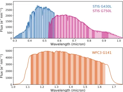
0.3 0.4 0.5 0.6 0.7 0.8 0.9 1.0 0 500 1000 1500 2000 2500 3000 _{STIS G430L} STIS G750L Wavelength (micron) Flu x ( e nm 1) 1.0 1.1 1.2 1.3 1.4 1.5 1.6 1.7 0 1000 2000 3000 4000 5000 _{WFC3 G141} Wavelength (micron) Flu x ( e nm 1)

Figure 1. Example spectra for the G430L and G750L gratings (top panel), and the G141 grism (bottom panel). Dark and light vertical bands indicate the wavelength channels adopted for the spectroscopic lightcurves.

2. OBSERVATIONS AND DATA REDUCTION

We observed three primary transits of WASP-121b using HST/STIS as part of the Panchromatic Comparative Exoplanet Treasury (PanCET) survey (Program 14767; P.I.s Sing and L´opez-Morales). This was comprised of two visits made on 2016 Oct 24 and 2016 Nov 6 with the G430L grating, and one visit made on 2016 Nov 12 with the G750L grating. In what follows, we shall refer to the first and second G430L visits as the G430Lv1 and G430Lv2 datasets, respectively. For all three STIS visits, the target was observed for 6.8 hours, covering five consecutive HST orbits. Observations were made using the widest available slit (52 × 2 arcsec) to minimize slit losses and the detector gain was set to 4 e−1/DN. Overheads were reduced by only reading out a 1024×128 pixel subarray containing the target spectrum. Exposure times of 253 s and 161 s were used for the G430L and G750L observations, respectively. We also took a short 1 s exposure at the start of each HST orbit for both gratings, but discarded these exposures in the subsequent analysis. This was done because STIS observations typically suffer from a systematic in which the first exposure of each HST orbit has anomalously lower counts relative to the immediately-following exposures (e.g.Evans

et al. 2013; Nikolov et al. 2014, 2015; Sing et al. 2015) and we wanted to minimize

the integration time lost to this effect. With this observing setup, we acquired a total of 48 science exposures for each G430L visit and 70 science exposures for the G750L visit.

The STIS datasets were reduced following the methodology described in Nikolov

et al. (2014, 2015). Raw data frames were bias-, dark-, and flat-corrected using the

CALSTIS pipeline (v3.4) with relevant calibration frames. Cosmic ray events and pixels flagged as ‘bad’ by CALSTIS were removed and interpolated over. Overall, we found ∼ 4% of pixels were affected by cosmic rays for all visits with a further ∼ 5%

Evans et al. 2.0 1.5 1.0 0.5 0.0

Flux change (%)

x (

un

itl

es

s)

Time from mid-transit (h)

y (

un

itl

es

s)

Time from mid-transit (h)

G750L

4 2 0 2

Time from mid-transit (h)

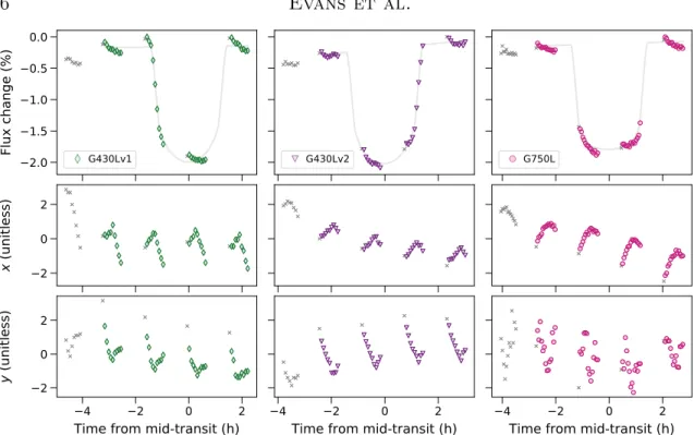
Figure 2. (Top row) Raw white lightcurves for the G430Lv1, G430Lv2, and G750L datasets. Gray lines show the best-fit transit signals with linear baseline trends. (Middle row) Dispersion drift variable for each dataset. (Bottom row) Cross-dispersion drift variable for each dataset. In all panels, colored symbols indicate data points that were included in the analysis and gray crosses indicate those that were excluded for reasons explained in the main text. The two drift variables are unitless as they have been standardized, i.e. mean subtracted and normalized by their standard deviations.

flagged as bad by CALSTIS. To extract spectra from the cleaned 2D frames, we used the IRAF procedure apall with aperture radii of 4.5, 6.5, 8.5, and 10.5 pixels for both the G430L and G750L datasets. The dispersion axis was mapped to a wavelength solution using the x1d files produced by CALSTIS.

In addition to the STIS data, a single primary transit of WASP-121b was observed on 2016 Feb 6 with the G141 grism (Program 14468; P.I. Evans). This dataset was originally published inEvans et al. (2016), to which the reader is referred for further details.

Example G430L, G750L, and G141 spectra are shown in Figure 1.

3. WHITE LIGHTCURVE ANALYSES

White lightcurves were constructed for each dataset by summing the flux of each spectrum across the full dispersion axis. The resulting lightcurves are shown in the top row of Figure 2. As in our previous work (Evans et al. 2013,2016, 2017), we fol-lowed the methodology outlined by Gibson et al. (2012) and treated each lightcurve as a Gaussian process (GP). Under this approach, the posterior likelihood is described by a multivariate normal distribution of the form N (d | µ, K + Σ), where: d is an N -length vector containing the flux measurements; µ is a vector containing the de-terministic mean function; K is an N × N matrix describing the correlations between

data points; and Σ is an N × N diagonal matrix containing the squared white noise uncertainties, σ2

j, for each data point j = 1, . . . , N .

For the mean function, we adopted aMandel & Agol(2002) transit model multiplied by a linear trend in time (t) of the form c0+ c1t. We assumed a circular orbit with

a period (P ) of 1.2749255 days (Delrez et al. 2016). We allowed the normalized planet radius (Rp/R?) and transit mid-time (Tmid) to vary as free parameters with

uniform priors. As described in Section3.1, we first performed fits with the normalized semimajor axis (a/R?) and impact parameter (b) allowed to vary as free parameters,

both with uniform priors. Then, as described in Section 3.2, we fixed a/R? and b to

their weighted-mean values and repeated the fitting.

In all fits, we assumed a quadratic limb darkening law and treated both coefficients (u1, u2) as free parameters. We first estimated values for u1 and u2 by fitting to the

limb darkening profile of a stellar model over the appropriate bandpass. Specificially, we used a 3D stellar model from the STAGGER grid (Magic et al. 2013) with T? =

6500 K, log₁₀g = 4 cgs, and [Fe/H] = 0 dex, as this was the grid point closest to the properties of the WASP-121 host star (T? = 6460 ± 140 K, log10g = 4.242 ± 0.2 cgs,

[Fe/H] = +0.13±0.09 dex;Delrez et al. 2016). We then applied broad normal priors to u1 and u2 in the model fitting, with means set to these estimated values and standard

deviations of 0.6, providing plenty of flexibility for the model to be optimized. For the GP covariance matrix K, we adopted a squared-exponential kernel1 with three input variables that it is reasonable to assume could correlate with the instru-mental systematics: namely, HST orbital phase (φ), dispersion drift (x), and cross-dispersion drift (y). This resulted in four free parameters for each dataset: namely, the covariance amplitude (A) and correlation length-scales (Lk) for each input

vari-able, k = {φ, x, y}. For the white noise matrix, Σ, we adopted the formal photon noise values σj multiplied by a rescaling factor (β) which was allowed to vary as a free

parameter. The latter affords some flexibility to handle high-frequency systematics that are pseudo-white-noise in nature, which would otherwise bias the model toward impractically small Lk values.

For the GP covariance amplitude A, we adopted Gamma priors of the form p(A) ∝

e−100A, to favor smaller correlation amplitudes. This can help prevent a small number

of outliers having a disproportionate influence on the inferred covariance amplitude. For the correlation length scales Lk, we followed previous studies (e.g. Evans et al.

2017; Gibson et al. 2017) and fit for the natural logarithm of the inverse correlation

length scales ln ηk = ln L−1_k , adopting uniform priors for each. In practice, this favors

longer correlation length scales, with the intention of capturing the lower-frequency systematics present in the data, as these are most degenerate with the planet signal. Higher-frequency systematics can be accounted for through the β parameter, for which

1 _{We refer the reader to previous studies such as Gibson et al. (2012), Evans et al.(2013), and}

Evans et al.

0.00 0.05 0.10 0.15 0.20

3.70

3.75

3.80

3.85

3.90

3.95

b = acos(i)/R

a/

R

HST STIS G430L

HST STIS G750L

HST WFC3 G141

HST weighted-mean

Delrez et al. (2016)

0.121

0.122

0.123

0.124

R

/R

0.121

0.122

0.123

0.124

R

/R

HST weighted-mean values:

a/R = 3.86 ± 0.02

b = 0.06 ± 0.04

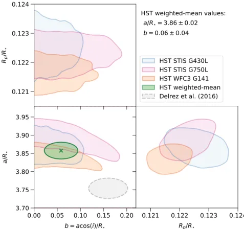
Figure 3. Posterior distributions for Rp/R?, a/R?, and b obtained from the white lightcurve

analyses described in Section3.1. Blue, pink, and orange regions indicate smoothed contours containing 68% of MCMC samples for the G430L, G750L, and G141 analyses, respectively. Green region indicates the weighted-mean of the HST posterior distributions and gray region indicates the 1σ range reported byDelrez et al. (2016).

we adopted a normal prior with mean of 1 and standard deviation of 0.2, to favor values close to the formal photon noise.

We modeled the white lightcurves for G430L, G750L, and G141 separately. For the G430L lightcurves, we assumed Rp/R?, a/R?, and b were the same for both visits,

while allowing Tmid, β, A, ln ηφ, ln ηx, and ln ηy to vary separately for each visit.

The posterior distributions were marginalized using affine-invariant Markov chain

Monte Carlo (MCMC), as implemented by the emcee Python package (

Foreman-Mackey et al. 2013). In all fits, we randomly distributed five groups of 150 walkers

throughout the parameter space and allowed them to run for 100 steps to locate the peak of the posterior distribution. We then re-initialized the five groups of 150 walkers in a tighter ball around this peak and allowed them to run for 500 steps, of which we discarded the first 250 steps as burn-in and combined the remaining 250 steps into a single chain for each walker group. At this point, a comparison of the chains from each walker group confirmed that they appeared well-mixed and converged, with Gelman-Rubin statistic values within 2% of unity for each free parameter (Gelman &

the STIS lightcurves produced using the different trial apertures (see Section 2), we obtained results consistent to within 1σ for the planet parameters (e.g. Rp/R?) and

report only those for the 8.5 pixel aperture.

3.1. a/R? and b allowed to vary

The purpose of the model fits in which a/R? and b were allowed to vary as free

parameters was to use the HST data to refine our estimates of these system properties. Previously, the only published measurements were those provided in the original discovery paper by Delrez et al. (2016), which reported a/R? = 3.754+0.023−0.028 and b =

0.160+0.040_−0.042. Figure3shows the posterior distributions obtained from our analyses for comparison, with values reported in Table1. We find good agreement for both a/R?

and b across our fits to the G430L, G750L, and G141 white lightcurve datasets. Taking the arithmetic weighted-mean of these results, we estimate a/R? = 3.86 ± 0.02 and

b = 0.06 ± 0.04, implying i = 89.1 ± 0.5 deg. We note that our HST results differ from those of Delrez et al. by 3.5σ for a/R?and 2σ for b. The reason for this disagreement is

unclear and will likely be resolved by additional transit observations that are currently planned or in the process of being analyzed (Evans et al., in prep.). For the present study, we note that the primary consequence of assuming slightly different values for a/R? and b will be to perturb the inferred values for Rp/R?. Importantly, this will be

a wavelength-independent effect and thus should not affect our interpretation of the atmospheric transmission spectrum. For this reason, and given the mutual agreement between the G430L, G750L, and G141 datasets, we adopt the HST weighted-mean values for a/R? and b in all subsequent lightcurve fits.

3.2. a/R? and b held fixed

Inferred values for Rp/R? can be biased by differences in the assumed values for

a/R? and b across datasets. For this reason, we held the latter parameters fixed

to the HST weighted-mean values determined in the previous section and repeated the white lightcurve analyses. This is physically motivated by the fact that the true values of a/R? and b should be constant across our datasets, and we are primarily

interested in wavelength-dependent variations of Rp/R? arising due to the planetary

atmosphere.

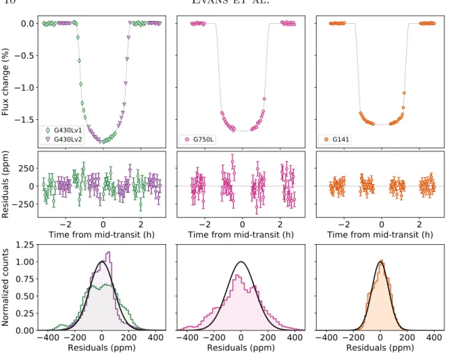
Figure 4 shows the best-fit transit models compared with the data after removing the systematics contribution inferred by the GP. The latter are shown separately in Figure5and Table1summarizes the posterior distributions. The resulting estimates for Rp/R?, u1, and u2 are all within 1σ of those obtained for the fits in which a/R?

and b were allowed to vary. Unsurprisingly, we obtain similar estimates for β, as this parameter is sensitive to high-frequency noise in the data that is unlikely to be significantly correlated with a/R? and b. The inferred β values imply scatters that are

∼ 20–40% and ∼ 10% above the photon noise floor for the STIS and WFC3 datasets, respectively. This is illustrated in Figure 4, which shows the model residuals. For

Evans et al.

1.5

1.0

0.5

0.0

Flux change (%)

2

0

2

250

0

250

Residuals (ppm)

Time from mid-transit (h)

400 200 0

200 400

Residuals (ppm)

0.00

0.25

0.50

0.75

1.00

1.25

Normalized counts

2

0

2

Time from mid-transit (h)

400 200 0

200 400

Residuals (ppm)

G141

2

0

2

Time from mid-transit (h)

400 200 0

200 400

Residuals (ppm)

Figure 4. White lightcurves for G430L, G750L, and G141 datasets analyzed in this study. (Top row) Relative flux variation after removing the systematics contribution inferred from the GP analyses (see Figure 5), with best-fit transit signals plotted as solid lines. (Middle row) Corresponding model residuals, with photon noise errorbars. (Bottom row) Normalized histograms of residuals obtained by subtracting from the data a random subset of GP mean functions obtained in the MCMC sampling. Solid black lines correspond to normal distributions with standard deviations equal to photon noise (i.e. prior to rescaling by the β factor described in the main text).

Tmid, we find the inferred values shift by ∼ 5–20 sec, but remain within ∼ 1σ of those

obtained for the fits in which a/R? and b were allowed to vary.

4. SPECTROSCOPIC LIGHTCURVE ANALYSES

Spectroscopic lightcurves were constructed by first summing the spectra of each dataset within the wavelength channels shown in Figure 1. Median channel widths were: 20 pixels (∼ 55 ˚A) for both G430L datasets; 20 pixels (∼ 98 ˚A) for the G750L dataset; and 4 pixels (∼ 186 ˚A) for the G141 dataset. Care was taken to avoid the edges of prominent stellar lines and to maintain similar levels of flux within each channel. Thus, subsets of the G430L and G750L channels were broader than these nominal widths. The resulting raw lightcurves for the STIS datasets are shown in Figures A.1-A.3.

We next generated common-mode (i.e. wavelength-independent) signals for each dataset by dividing the raw white lightcurves by the corresponding best-fit transit

3 2 1 0 1 2 3 0.1 0.0 0.1 Systematics (%)

G430Lv1

G430Lv2

Time from mid-transit (h)

Systematics (%)

G750L

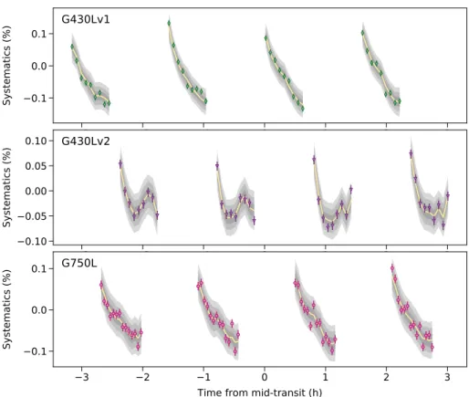
Figure 5. Systematics in the white lightcurves for G430L and G750L datasets. Effectively, these are the residuals after dividing the raw flux time series by the transit signals with linear baseline trends shown in Figure2. Yellow lines and gray shaded regions, respectively, show the means and 1σ, 2σ, and 3σ ranges of the best-fit GP distributions. Note that in practice the transit signal, linear baseline trend, and GP are fit simultaneously. The purpose of this figure is only to highlight the structure of the systematics.

signals obtained in Section 3 and shown in Figure 4. Each of the raw spectroscopic lightcurves were then divided by the resulting common-mode signals. Note that in addition to removing common-mode systematics, this latter step also has the ef-fect of dividing each spectroscopic lightcurve by the intrinsic scatter of the white lightcurve. However, this is acceptable, as the spectroscopic lightcurves have a larger intrinsic scatter than the white lightcurves: dividing white noise by lower-amplitude white noise should on average have zero net effect on the scatter of the resulting corrected lightcurves. Meanwhile, applying a common-mode correction of this nature – as opposed to dividing through by the best-fit systematics model from the white lightcurve fits – has the potential advantage of removing systematics in the spec-troscopic lightcurves that may not be captured by our white lightcurve systematics model. The common-mode corrected lightcurves for the STIS datasets are shown in Figures A.4-A.6.

To fit the spectroscopic lightcurves, we used the same approach as described in Section 3. The only exception was that we fixed Tmid to the best-fit values listed

in Table 1. Thus, for the spectroscopic transit signals, the free paramaters were the radius ratio (Rp/R?) and quadratic limb darkening coefficients (u1, u2). For the

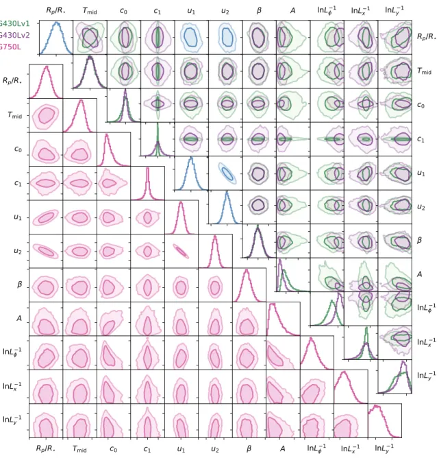
Evans et al. Rp/R Rp/R Rp/R Rp/R Tmid Tmid Tmid Tmid c0 c0 c0 c0 c1 c1 c1 c1 u1 u1 u1 u1 u2 u2 u2 u2 A A A A lnL 1 lnL 1 lnL 1 lnL 1 lnL_x1 lnL_x1 lnL_x1 lnL_x1 lnL 1 y lnL_y1 lnL_y1 lnL_y1 G430Lv1 G430Lv2 G750L

Figure 6. Posterior distributions obtained from the white lightcurve analyses described in Section 3.2. Top right panels show results for the joint analysis of both G430L visits and bottom left panels show results for the G750L analysis. Plotted contours contain 68% and 95% of the MCMC samples. Panels along the diagonal show marginalized posterior distri-butions. Note that Tmid, c0, c1, and β have been median-subtracted to allow both G430L

visits to be plotted on the same axes. The purpose of this figure is to visually illustrate correlations between model parameters. Numerical values for all parameter distributions are summarized in Table1.

G430L analysis, we fit both visits jointly with shared values for Rp/R?, u1, and u2,

as was done for the white lightcurve analysis. In all fits, we again accounted for systematics by fitting for a linear trend in t and a GP with {φ, x, y} as inputs to a squared-exponential covariance kernel. White noise levels were allowed to vary for each individual lightcurve via β rescaling parameters. Marginalization of the posterior

2 0 2 0.825 0.850 0.875 0.900 0.925 0.950 0.975 1.000 290-350nm 350-370nm 370-387nm 387-404nm 404-415nm 415-426nm 426-437nm 437-443nm 443-448nm 448-454nm 2 0 2 454-459nm 459-465nm 465-470nm 470-476nm 476-481nm 481-492nm 492-498nm 498-503nm 503-509nm 509-514nm 2 0 2 514-520nm 520-525nm 525-530nm 530-536nm 536-541nm 541-547nm 547-552nm 552-558nm 558-563nm 563-569nm 2 0 2 25000 2500 2 0 2 2 0 2 2 0 2 25000 2500 2 0 2 2 0 2 2 0 2 25000 2500 2 0 2 2 0 2 2 0 2 25000 2500 2 0 2 2 0 2 2 0 2 25000 2500 2 0 2 2 0 2 2 0 2 25000 2500 2 0 2 2 0 2 2 0 2 25000 2500 2 0 2 2 0 2 2 0 2 25000 2500 2 0 2 2 0 2 2 0 2 25000 2500 2 0 2 2 0 2 2 0 2 25000 2500 2 0 2 2 0 2

Time from mid-transit (h) Time from mid-transit (h) Time from mid-transit (h)

Relative flux

Residuals (ppm)

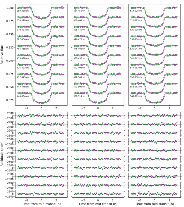
Figure 7. Spectroscopic lightcurves for the G430Lv1 and G430Lv2 datasets after removing the systematics contributions inferred from the GP analyses, with best-fit transit signals plotted as solid lines. Green triangles and purple diamonds correspond to the G430Lv1 and G430Lv2 datasets, respectively.

distributions was performed in the manner described above, using affine-invariant MCMC.

The best-fit transit signals and model residuals are shown in Figure7for G430L and Figure8for G750L. Figure9shows the systematics and GP fits for each spectroscopic lightcurve. Histograms of residuals are shown in Figures A.4-A.6. For the G141 spectroscopic lightcurve fits, the results were essentially identical to those presented

inEvans et al. (2016), so we do not duplicate them here. The only difference for the

Evans et al. 2 0 2 0.825 0.850 0.875 0.900 0.925 0.950 0.975 1.000 526-555nm 555-565nm 565-575nm 575-584nm 584-594nm 594-604nm 604-614nm 614-623nm 623-633nm 633-643nm 2 0 2 643-653nm 653-662nm 662-672nm 672-682nm 682-692nm 692-701nm 701-711nm 711-721nm 721-731nm 731-740nm 2 0 2 740-750nm 750-760nm 760-770nm 770-780nm 780-799nm 799-819nm 819-838nm 838-884nm 884-930nm 930-1025nm 2 0 2 25000 2500 2 0 2 2 0 2 2 0 2 25000 2500 2 0 2 2 0 2 2 0 2 25000 2500 2 0 2 2 0 2 2 0 2 25000 2500 2 0 2 2 0 2 2 0 2 25000 2500 2 0 2 2 0 2 2 0 2 25000 2500 2 0 2 2 0 2 2 0 2 25000 2500 2 0 2 2 0 2 2 0 2 25000 2500 2 0 2 2 0 2 2 0 2 25000 2500 2 0 2 2 0 2 2 0 2 25000 2500 2 0 2 2 0 2

Time from mid-transit (h) Time from mid-transit (h) Time from mid-transit (h)

Relative flux

Residuals (ppm)

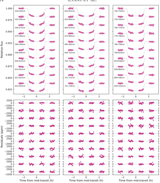
Figure 8. Similar to Figure7, but for the G750L spectroscopic lightcurves.

lightcurve analysis which gives Rp/R? = 0.1218 ± 0.0004 (Table 1), compared with

the previous estimate of Rp/R? = 0.1211 ± 0.0003 (Evans et al. 2016).2

As shown in Figure10, we obtain means and standard deviations for the inferred β values across spectroscopic channels of: 1.05±0.07 for the G430lv1 dataset; 1.06±0.09 for the G430Lv2 dataset; 1.05 ± 0.05 for the G750L dataset; and 1.02 ± 0.06 for the G141 dataset. The consistency of these results with β = 1 indicate that the GP models are broadly successful at marginalizing over the correlations in the lightcurves, implying in turn that degeneracies between the systematics and planet signal are

2_{The revised value for R}

p/R? within the G141 bandpass can be attribued to the updated values

0.25 0.00 0.25 0.25 0.00 0.25 0.25 0.00 0.25 0.25 0.00 0.25 0.25 0.00 0.25 0.25 0.00 0.25 0.25 0.00 0.25 0.25 0.00 0.25 0.25 0.00 0.25 0.25 0.00 0.25 0.25 0.00 0.25 0.25 0.00 0.25 0.25 0.00 0.25 0.25 0.00 0.25 0.25 0.00 0.25 0.25 0.00 0.25 0.25 0.00 0.25 0.25 0.00 0.25 0.25 0.00 0.25 0.25 0.00 0.25 0.25 0.00 0.25 0.25 0.00 0.25 0.25 0.00 0.25 0.25 0.00 0.25 0.25 0.00 0.25 0.25 0.00 0.25 0.25 0.00 0.25 0.25 0.00 0.25 0.25 0.00 0.25 2 0 2 0.25 0.00 0.25 2 0 2 2 0 2

Time from mid-transit (h) G430Lv1

Time from mid-transit (h) G430Lv2

Time from mid-transit (h) G750L

Spectroscopic lightcurve systematics (%)

Figure 9. Similar to Figure5, but showing the systematics and GP fits for the spectroscopic lightcurves. In all columns, wavelength increases from top to bottom.

Evans et al. 0.8 1.0 1.2 1.4 G430Lv1 G430Lv2 0.3 0.4 0.5 0.8 1.0 1.2 1.4 G750L 0.6 0.8 1.0 G141 1.2 1.4 1.6

Wavelength (micron)

Wavelength (micron)

Wavelength (micron)

, S

qu

ar

ed

E

xp

.

, M

at

er

n

=

3/

2

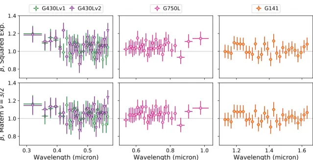
Figure 10. (Top row) Inferred white noise rescaling parameters β for the GP analyses adopting a squared-exponential covariance kernel. (Bottom row) The same, but for the GP analyses adopting a Mat´ern ν = 3/2 covariance kernel.

properly accounted for in our estimates of parameters such as Rp/R?, which we are

primarily interested in.

To investigate the sensitivity of our results to the choice of covariance kernel, we re-peated the spectroscopic lightcurve fitting using the Mat´ern ν = 3/2 kernel, which can be more suitable for modeling high-frequency signals than the squared-exponential kernel (e.g. see Gibson et al. 2012). For all channels, we found the inferred Rp/R?

values remained unchanged to well-within 1σ, regardless of which covariance kernel was used. However, the β values inferred using the Mat´ern ν = 3/2 kernel were on average slightly closer to unity, as illustrated in Figure 10. This suggests some of the channels may contain high-frequency noise that can be suitably accounted for either by inflating the white-noise level above the photon noise floor via β > 1 or by employing a covariance kernel with enough flexibility to marginalize over signals of this nature, such as the Mat´ern ν = 3/2. Given the results for Rp/R? are found to

be insensitive to the choice of covariance kernel, we adopt those obtained using the squared-exponential for the remainder of this paper.

The corresponding posterior distributions for Rp/R?, u1, and u2 are summarized

for each STIS dataset in Tables 2 and 3. The median uncertainties on Rp/R? are

800 ppm for G430L, 900 ppm for G750L, and 500 ppm for G141, which translates to uncertainties on the transit depth (Rp/R?)2 of approximately 200 ppm, 220 ppm and

125 ppm, respectively. For comparison, a change in the effective planetary radius of one atmospheric pressure scale height H corresponds to a transit depth variation of ∼ 150–200 ppm for WASP-121b, assuming average limb temperatures in the range of 1500–2000 K, a planetary surface gravity of 940 cm s−2, and an atmospheric mean molecular weight of µ = 2.22 atomic mass units (i.e. equal to that of Jupiter).

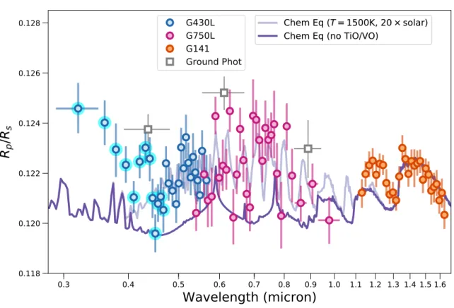
0.3 0.4 0.5 0.6 0.7 0.8 0.9 1.0 1.1 1.2 1.3 1.4 1.5 1.6 0.118 0.120 0.122 0.124 0.126 0.128

Wavelength (micron)

R

p

/R

s

G430L

G750L

G141

Ground Phot

Chem Eq (T = 1500K, 20 × solar)

Chem Eq (no TiO/VO)

Chem Eq (T = 1500K, 20 × solar)

Chem Eq (no TiO/VO)

Figure 11. Transmission spectrum for WASP-121b obtained using STIS and WFC3 (col-ored circles) and ground-based photometry from Delrez et al. (2016) (unfilled squares). Note that the latter are taken from the re-analysis of Evans et al. (2016), although very similar results were obtained by Delrez et al. Light blue halos indicate the subset of G430L data that we refer to as the blue data in the main text. Two forward models assuming chemical equilibrium are also shown, both with a temperature of 1500 K and 20× solar metallicity. One model includes TiO/VO opacity (light purple line) and the other does not include TiO/VO opacity (dark purple line).

5. DISCUSSION

The measured transmission spectrum is shown in Figure 11 and has a number of

notable features. In particular, the G430L data exhibit a steep rise toward shorter wavelengths from ∼ 0.47 µm, where Rp/R? ∼ 0.121, to ∼ 0.28 µm, where Rp/R? ∼

0.125. This corresponds to a change in effective planetary radius of approximately five pressure scale heights. At longer optical wavelengths covered by the G430L and G750L gratings (∼ 0.47–1 µm), Rp/R? is measured to vary across spectroscopic

channels, implying a wavelength-dependent atmospheric opacity. Within some of these optical channels, the atmospheric opacity is found to be even higher than that measured within the H2O band at 1.4 µm, which is detected in the G141 bandpass

(Evans et al. 2016).

Figure 11 also shows the Rp/R? values measured using ground-based photometry

in the B, r0, and z0 bandpasses. The latter were originally reported by Delrez et al.

(2016) and an independent analysis of the same lightcurves was presented by Evans

et al.(2016). Both studies obtained similar estimates for Rp/R?in each bandpass that

Evans et al.

for this tension. As noted above, updated values for a/R? and b were used in the

lightcurve fits of the present study. However, for the G141 dataset, this had the effect of shifting the mean Rp/R? value to a higher value from 0.1211 ± 0.0003 (Evans

et al. 2016) to 0.1218 ± 0.0004 (Table 1). A similar upward shift for the

ground-based photometry would make those data more discrepant relative to the HST data. Alternatively, during the photometry data reduction, effects such as aperture light-losses or an over-estimated background may have artificially deepened the transit signals, resulting in Rp/R?estimates above the true values. Another more speculative

possibility is intrinsic variability of the atmosphere from epoch to epoch. For example,

Parmentier et al. (2013) report a 3D GCM study showing that significant variations

in passive tracer abundances over ∼ 100 day timescales are possible at the planetary limb of hot Jupiters. As those authors note, if this occurs for strongly-absorbing species such as TiO and VO, it could have significant implications for transmission spectra measured at different epochs. Indeed, the ground-based photometry and HST STIS observations were separated by over 100 days. However, the current data are insufficient to test this theory, and we consider it more likely that the difference is due to some unaccounted-for systematic in the ground-based photometry.

To evaluate the robustness of the HST transmission spectrum, we performed a number of tests, full details of which are reported in Appendix B. First, we find that the measured transmission spectrum is insensitive to our treatment of limb darkening. Second, we investigated the inclusion of time t as an additional GP input variable in the lightcurve fits and obtain very similar results to those reported here. Third, for the G430L data, we find that the measured transmission spectrum is repeatable when each of the two visits are analyzed separately. Fourth, we conclude that stellar activity is unlikely to have significantly affected the measured transmission spectrum, based on: (1) the lack of photometric variability and modest X-ray flux of the WASP-121 host star; (2) the epoch-to-epoch repeatability of the G430L datasets; (3) the good level of agreement obtained across the overlapping wavelength range of the G430L and G750L datasets; and (4) the inability of unocculted spots to explain the shape of the measured spectrum under reasonable assumptions. In the following sections, we therefore seek to interpret the measurements shown in Figure 11as the signal of the planetary atmosphere.

5.1. Rayleigh scattering and a gray cloud-deck

The signature of aerosol scattering is ubiquitous in observations of exoplanet at-mospheres (e.g. Pont et al. 2008; Kreidberg et al. 2014; Nikolov et al. 2014, 2015;

Sing et al. 2015). For hot Jupiter transmission spectra, this is unsurprising given

the large number of refractory species expected to condense at the temperatures and pressures characteristic of these atmospheres (e.g. Woitke et al. 2018), as well as the highly-sensitive nature of the grazing geometry to even trace opacity sources (Fortney 2005). Indeed, the rise in opacity toward shorter wavelengths that we measure for

WASP-121b is somewhat reminiscent of transmission spectra previously obtained for other hot Jupiters, which can be explained by Rayleigh scattering due to high-altitude layers of submicron aerosols (Sing et al. 2016). In addition, an optically-thick cloud deck could act as a gray opacity source, if present at low pressures.

We investigated how well the WASP-121b transmission spectrum can be explained by aerosols by first fitting simple Rayleigh scattering and cloud deck models to the STIS data spanning the G430L and G750L gratings. For the Rayleigh component, we followed the methodology outlined by Lecavelier Des Etangs et al.(2008) (L08), who provide relations between the slope of the transmission spectrum and the atmospheric temperature, under the assumption of scattering particles distributed uniformly with pressure. For the cloud deck component we assumed a wavelength-independent opac-ity, implemented as a horizontal flat line in Rp/R? that was allowed to float vertically

relative to other spectral features in the transmission spectrum. For this initial anal-ysis, we excluded the G141 dataset, as it exhibits a clear spectral feature due to H2O,

which would add additional complexity to the model. This is addressed in Section

5.4, where we perform a free-chemistry fit to the combined STIS+WFC3 dataset that includes opacity due to both gas-phase species and aerosols.

Our best-fit model combining a Rayleigh slope with cloud-deck is shown in Fig-ure 12. It provides a poor fit to the data, with a reduced χ2 of 1.8 for 57 degrees of freedom, allowing us to exclude it at 3.7σ confidence. This is due to the in-ability of a featureless cloud deck to explain the optical data across the 0.47–1 µm wavelength range. Furthermore, the temperature inferred from the Rayleigh slope is 6980 ± 3660 K, which is improbably high for the atmospheric pressures probed in transmission. For instance, if WASP-121b absorbs all incident radiation on its day-side hemisphere (i.e. the Bond albedo is zero), then the substellar point would have

a temperature of T?/pa/R? ∼ 3280 K and the day-night boundary probed by the

transmission spectrum should be considerably cooler. Furthermore, at such high tem-peratures, no condensates are expected to exist and molecules should be thermally dissociated, including H2.

To be conservative, we also tried dividing the NUV-optical data into different wave-length sections and fitting them one at a time. For convenience, we will refer to these subsets as the blue (0.3–0.47 µm) and red (0.47–1 µm) data. In principle, a good fit to one or both of these datasets separately should be easier to achieve than a good joint fit, as the models need not be self-consistent.

First, we fit a Rayleigh profile to the blue data, as this is where the transmission spectrum exhibits a strong slope. Although we obtain a better statistical fit with a reduced χ2 _{of 1.6 for 10 degrees of freedom (Figure 12), the inferred temperature}

remains implausibly high at 6810 ± 1530 K. Given this, we conclude that the rise in the measured transmission spectrum toward NUV wavelengths is too steep to be explained by scattering out of the transmission beam. Instead, it would suggest the presence of one or more significant NUV absorbers in the upper atmosphere of

WASP-Evans et al. 0.3 0.4 0.5 0.6 0.7 0.8 0.9 1.0 0.118 0.120 0.122 0.124 0.126 0.128

Wavelength (micron)

R

p

/R

s

G430L

G750L

Chem Eq (T = 1500K, 20 × solar)

Rayleigh blue (T = 6810 ± 1530K)

Rayleigh+Cloud (T = 6980 ± 3660K)

Chem Eq (T = 1500K, 20 × solar)

Rayleigh blue (T = 6810 ± 1530K)

Rayleigh+Cloud (T = 6980 ± 3660K)

Wavelength (micron)

R

p

/R

s

G430L

Excluded

Chem Eq (T = 1500K, 20 × solar)

SH (T = 1500K, vmr = 100ppm)

SH (T = 2000K, vmr = 20ppm)

Chem Eq (T = 1500K, 20 × solar)

SH (T = 1500K, vmr = 100ppm)

SH (T = 2000K, vmr = 20ppm)

Figure 12. Similar to Figure 11, but showing only the STIS data. (Top panel) Rayleigh scattering fit to the NUV data only (green line) and a hybrid Rayleigh+cloud model fit to the complete STIS dataset (yellow line). Although Rayleigh scattering gives a good fit to the NUV data, it requires invoking an unphysically high temperature. The Rayleigh+cloud model is ruled out at 3.7σ confidence, due to the opacity variations measured across optical wavelengths. (Bottom panel) Models illustrating the expected opacity contribution due to SH for temperatures of 1500 K and 2000 K with volume mixing ratios 100 ppm and 20 ppm, respectively (brown lines).

121b, assuming the slope is indeed a feature of the planetary spectrum and not caused by an uncorrected systematic effect in the data.

Second, we tried fitting a gray cloud deck to the G430L and G750L data, with the blue G430L subset excluded. For this scenario (not shown in Figure 12), we obtain a reduced χ2 _{of 1.9 for 51 degrees of freedom, which formally rules it out}

at 3.8σ confidence. Alternatively, if the Rp/R? uncertainties for these optical data

have been uniformly underestimated by ∼ 30%, this gray cloud scenario would only be excluded at ∼ 1σ confidence. However, lacking any reason to doubt our inferred Rp/R? uncertainties, we propose instead that the optical data exhibit significant

spectral variations that cannot be explained by a gray cloud deck.

5.2. Forward model comparison with optical-NIR data

The results of the previous section imply the transmission spectrum of WASP-121b exhibits significant wavelength-dependent opacity variations across the ∼ 0.47–1 µm wavelength range. To explore this further, we used the ATMO code (Amundsen et al.

2014;Drummond et al. 2016;Goyal et al. 2018;Tremblin et al. 2015,2016) to generate

a small grid of aerosol-free atmosphere models spanning temperature and metallicity, assuming isothermal pressure-temperature (PT) profiles and chemical equilibrium abundances. Specifically, our grid consisted of temperatures ranging from 1000 K to 2700 K in 100 K increments, each evaluated for metallicities of 0.1×, 1×, 10×, 20×, 30×, 40×, and 50× solar. ATMO solves for the gas-phase and condensed-phase chemical equilibrium mole fractions for a given pressure, temperature, and set of elemental abundances (Drummond et al. 2016). For the results presented here we consider local condensation, such that the chemistry calculation in each model pressure level is entirely independent of all other pressure levels. We do not account for rainout chemistry, under which condensation deeper within the atmosphere depletes elemental abundances at lower pressures levels (Burrows & Sharp 1999; Madhusudhan et al.

2011; Mbarek & Kempton 2016). Rainout could be important in the atmosphere of

WASP-121b, but we defer investigation of this effect to future work that includes a more realistic treatment of the PT profile than the isothermal assumption made here. Finally, we applied uniform vertical offsets to Rp/R? for each model in order to

optimize the match to the data. No further tuning of the models was performed. None of these equilibrium models are able to explain the absorption at wavelengths shortward of 0.47 µm, nor the G141 bump between wavelengths of 1.15–1.3 µm. We discuss these latter two components of the transmission spectrum further in Sections

5.3and5.4, respectively. For the remaining data – namely, the STIS data spanning the 0.47–1 µm wavelength range and the WFC3 data covering the H2O band centered at

1.4 µm – we find a good match is obtained for the model with a temperature of 1500 K and metallicity of 20× solar (Figure11), which has a reduced χ2 _{of 1.0 for 69 degrees}

Evans et al. 0.5 1.0 1.5 0.118 0.119 0.120 0.121 0.122 0.123 0.124

Wavelength (micron)

R

/R

Volume mixing ratio

log

[ P

(b

ar

) ]

Figure 13. (Left panel ) Individual contributions to the transmission spectrum due to the major radiatively-active species in the best-match forward model shown in Figure 11, i.e. chemical equilibrium for T = 1500 K and 20× solar metallicity. Note that continuum opacity due to gas-phase species such as H2 and He is not shown. (Right panel ) Corresponding

pressure-dependent abundances.

with metallicities of 10× and 30× solar. These metallicities are broadly consistent with predictions for a 1.18MJ planet such as WASP-121b (Thorngren et al. 2016).

Aside from collision-induced asorption and gas-phase Rayleigh scattering, the pri-mary opacity sources of these models are Na and VO at optical wavelengths and H2O

at NIR wavelengths. This is illustrated in Figure 13, which shows a break-down of the opacity sources in the best-matching chemical equilibrium model. Interestingly, opacity due to TiO is not as significant as VO in the optical, despite Ti being approxi-mately an order of magnitude more abundant than V for solar elemental composition

(Asplund et al. 2009). This occurs because for a given pressure, the condensation

of Ti species commences at higher temperatures than for V species (e.g. Burrows

& Sharp 1999; Woitke et al. 2018). The isothermal temperature of the best-match

model (i.e. 1500 K) is less than the condensation temperature of both Ti3O5(s) and

V2O3(s), meaning that these are the dominant forms of Ti and V in the model,

re-spectively. However, since the isothermal temperature is closer to the VO(g)/V2O3(s)

condensation temperature than the TiO(g)/Ti3O5(s) condensation temperature, the

abundance of VO(g) is larger than for TiO(g).

In contrast, Lodders (2002) found that calcium titanates (e.g. CaTiO5) – which

are not currently included in ATMO – are likely to be the first Ti-bearing

conden-sates to form. Furthermore, arguing from trends in solar system meteorite data

and M/L dwarf spectra, Lodders notes that V will likely condense in solid solution with the calcium titanates, resulting in VO gas-phase depletion commencing at the same temperature as TiO gas-phase depletion. However, for hot Jupiters, Ti and V condensation may depend on condensation and mixing timescales, both vertical and horizontal, that are very different to the protostellar nebula and M/L dwarfs. Such

details are complex and beyond the scope of the present study. At this stage, we simply note that VO absorption is favored by these HST data for WASP-121b, with no evidence for significant TiO absorption, an interpretation that is corroborated by the free-chemistry retrieval presented in Section 5.4 below.

We also note that the best-matching forward model temperature of 1500 K is sub-stantially cooler than that of the dayside photosphere, which is inferred to be ∼ 2700 K from secondary eclipse measurements (Evans et al. 2017). Such a large temperature difference between the dayside photosphere probed during secondary eclipse and the upper atmosphere of the day-night limb probed during primary transit is in fact broadly in line with predictions of 3D general circulation models of ultra-hot Jupiters (e.g. Kataria et al. 2016). Furthermore, the best-match temperature of 1500 K is likely to be at the lower end of the plausible range, because, as noted above, the forward models we consider here do not include rainout chemistry. Rainout chem-istry will likely result in VO condensing at higher temperatures, as the abundance of VO in the upper atmosphere would be determined by the atmospheric temperature profile at higher pressures where the condensation temperature is also higher. Since the appearance or disappearance of VO spectral bands is primarily what determines the ability of our forward models to match the data (Figure11), forward models with rainout chemistry would consequently tend to favor higher temperatures. As noted above, we do not consider models with rainout here, as the details will be highly sensitive to the atmospheric PT profile at pressures > 0.1 bar, which is unconstrained by the current data.

5.3. Absorption at NUV wavelengths

We now consider the steep rise in the transmission spectrum at wavelengths short-ward of ∼ 0.47 µm. As explained in Section 5.1, we consider it unlikely that this feature can be explained by Rayleigh scattering due to gas-phase species such as H2

or high-altitude aerosols. In addition, our chemical equilibrium models presented in Section 5.2 do not predict significant absorption above the H2 continuum at these

wavelengths. Nonetheless, we find the rise of the transmission spectrum at NUV wavelengths is empirically repeatable. It is recovered by our analysis when the spec-troscopic lightcurves for the two G430L visits are fit jointly and also when they are each fit individually (see Section B.4).

One candidate absorber is the mercapto radical, SH, comprised of a sulfur atom and a hydrogen atom. Indeed, SH was predicted byZahnle et al.(2009) (Z09) to be a strong NUV absorber in hot Jupiter atmospheres. Using a 1D photochemical kinetics code, Z09 found the abundance of SH may peak at pressures around ∼ 1–100 mbar in typical hot Jupiter atmospheres, with a mixing ratio of ∼ 10 ppm (see Figure 2 of Z09). At these pressures, H2S is the most abundant sulfur-bearing phase under

chemical equilibrium (Visscher et al. 2006), while atomic H and S are also available due to photodissociation of molecules such as H2 and H2O. The production of SH

Evans et al. 0.3 0.4 0.5 0.6 0.7 0.8 0.9 1.0 1.1 1.2 1.3 1.4 1.5 1.6 10 30 10 28 10 26 10 24 10 22 10 20 10 18 10 16 10 14 10 12

Wavelength (micron)

Cr

os

s-s

ec

tio

n

(cm

p

er

p

ar

tic

le)

Key to SH absorption cross-sections:

H2O

VO

Na

electronic (T = 1500K)

electronic (T = 2000K) ro-vibrational (T = 1500K)ro-vibrational (T = 2000K)

Figure 14. Absorption cross-sections for SH. Electronic transitions are fromZahnle et al.

(2009) and rotational-vibrational transitions are from ExoMol (Yurchenko et al. 2018). Cross-sections for H2O, VO, and Na are also shown, weighted by the relative abundances

implied by the model shown in Figure13.

then proceeds through numerous chemical pathways involving H2S, H, and S (Z09;

see also Zahnle et al. 2016).

To explore whether or not SH can explain the observed NUV absorption, we per-formed a simple fit to the 13 shortest-wavelength data points of the transmission spectrum, spanning the 0.3–0.47 µm wavelength range (i.e. the blue G430L data sub-set indicated by light blue halos in Figures11and12). As in Section5.1, we followed the methodology outlined in L08. We computed the change in relative planetary ra-dius due to SH absorption, adopting a planetary surface gravity g = 940 cm s−2 and stellar radius R? = 1.458R (Delrez et al. 2016). We also assumed µ = 2.22 atomic

mass units (see Section 4) and set Rp/R? = 0.120 as the altitude where H2 becomes

optically thick at grazing geometry for a wavelength of λ0 = 350 nm (Figure 11),

corresponding to a planetary radius of Rp = 1.702 RJ. This in turn translates to an

atmospheric pressure of ∼ 20 mbar, assuming a temperature of ∼ 1500–2000 K and an H2 scattering cross-section of σ0 = 3.51 × 10−27cm2molecule−1 for λ0 = 350 nm

(see Section 4.1 of L08; also, Sing et al. 2016). Having thus established the pres-sure scale, we took the temperature-dependent absorption cross-sections for SH and varied the mixing ratio to optimize the match to the NUV transmission spectrum using Equation 1 of L08. For the SH cross-sections, we combined those derived by Z09 with those recently published by the ExoMol project (Yurchenko et al. 2018). Specifically, the Z09 cross-sections were generated from transitions of the lowest five vibrational levels of the ground electronic state X2Π to the lowest three vibrational

SO S2 SH S H2S T Pre ssu re [ b a rs] 10−8 10−6 10−4 10−2 1

Volume Mixing Ratio

10−9 10−8 10−7 10−6 10−5 10−4 10−3

Temperature [K]

1000 2000 3000

Figure 15. Abundance predictions for important sulfur species assuming 20× solar metal-licity and Kzz = 109cm2s−1. Dashed green line indicates the adopted PT profile, based on

the limb average of a 3D GCM for WASP-121b (Kataria et al., in prep). Calculations were performed using the photochemical kinetics code ofZahnle et al. (2009), assuming a planet with a hydrogen-dominated atmosphere orbiting an F6V host star at the same distance as WASP-121b.

levels of the upper electronic state A2Σ+ _{(without predissociation), and exhibit a}

strong NUV signature. These transitions are not considered in the ExoMol cross-sections, which only account for rotational-vibrational transitions. Both the Z09 and ExoMol cross-sections are shown in Figure 14.

The results of this process are shown in Figure 12. We obtain respectable matches to the data with mixing ratios of ∼ 100 ppm and ∼ 20 ppm, respectively, for the

T = 1500 K and T = 2000 K absorption cross-sections of Z09. For comparison,

Figure 15 shows predicted abundances from the photochemical kinetics code of Z09 for a planet similar to WASP-121b with 20× solar metallicity and vertical mixing parameter Kzz = 109cm2s−1. We find abundances of ∼ 20–100 ppm are plausible

for SH across the bar to mbar pressure range probed by the transmission spectrum, lending some credibility to the hypothesis that it could be the mystery NUV absorber. However, as stressed by Z09, the SH cross-sections remain subject to considerable uncertainty, due to the paucity of available experimental data. This, combined with the low spectral resolution of the G430L data, prevent us from conclusively confirming

or ruling out SH at the present time. Other sulfur-bearing compounds that are

likely to be abundant, such as SiS, have strong features at NUV wavelengths but remain poorly modeled. Lothringer et al. (2018) have also flagged gas-phase Fe as an important NUV absorber in ultra-hot Jupiter atmospheres, although we find it

Evans et al.

is unable to account for the measured signal in the present dataset – at least under assumptions of equilibrium chemistry for pressures > 10−5bar – as it was included in the ATMO forward models described in Section 5.2 (see Figure 13).

Regardless of the identity of the putative NUV absorber, it likely provides signif-icant heating of the upper atmosphere. For instance, across the 0.3–0.47 µm wave-length range, the mean SH absorption cross-section varies from ∼ 10−16 to 10−22 cm2_molecule−1 _{(Figure 14). Assuming a mixing ratio of ∼ 10 ppm, in line with our}

above estimates, this implies a mean atmospheric opacity (i.e. absorption cross-section × mixing ratio) of ∼ 10−24_cm2_molecule−1 _{at the pressures probed in transmission.}

We find incorporating such an absorber into the 1D radiative-convective atmosphere model of Marley and collaborators (e.g. Marley & McKay 1999; Marley et al. 2002;

Fortney et al. 2008;Saumon & Marley 2008;Marley et al. 2012) would likely heat the

atmosphere of WASP-121b by ∼ 500 K at mbar pressures. Such heating could, for example, help maintain optical absorbers such as VO and TiO in the gas phase, which in turn would provide further heating of the upper atmosphere. Properly account-ing for effects such as these may be important for accurate modelaccount-ing of planetary circulation and energy budgets.

Absorption of incident UV flux exceeding that predicted by models has also been observed in solar system atmospheres. Two well-known examples are Venus and Jupiter. On Jupiter, a broad reflectivity dip near 0.3 µm has been attributed to a high-altitude dust or haze (Owen & Sagan 1972;Axel 1972). The composition of this chromophore is still not known and is generally attributed to some disequilibrium combination of S, N, C, and P species (for a fuller discussion see West et al. 2004). Likewise on Venus, dark markings in the atmosphere at UV wavelengths remain poorly understood, well over four decades after their discovery (e.g., Esposito et al. 1997). These features have also been attributed to some disequilibrium – perhaps S-bearing – absorber (but seePollack et al. 1980).

5.4. Retrieval analysis of optical-NIR data

In addition to comparing the data with predictions of forward models that assume chemical equilibrium (Section 5.2), we performed a free-chemistry retrieval analysis. For these calculations, we treat the abundances of the radiatively-active chemical species as free parameters in the model, rather than solving for the chemical equi-librium abundances at a given temperature. As for the forward models, this was done using ATMO, which can compute transmission spectra for any given atmospheric composition and PT profile. ATMO has previously been used for retrieval analyses of transmission spectra (Wakeford et al. 2017, 2018) and thermal emission spectra

(Evans et al. 2017).

Since ATMO does not currently include any opacity sources that can explain the steep rise observed at NUV wavelengths (Figure 11), we restricted the retrieval to optical-NIR wavelengths longward of 0.47 µm. We assumed an isothermal PT profile