HAL Id: hal-02792243
https://hal.inrae.fr/hal-02792243
Submitted on 5 Jun 2020
HAL is a multi-disciplinary open access archive for the deposit and dissemination of sci-entific research documents, whether they are pub-lished or not. The documents may come from teaching and research institutions in France or abroad, or from public or private research centers.
L’archive ouverte pluridisciplinaire HAL, est destinée au dépôt et à la diffusion de documents scientifiques de niveau recherche, publiés ou non, émanant des établissements d’enseignement et de recherche français ou étrangers, des laboratoires publics ou privés.
Veliborka Josipovic
To cite this version:
Veliborka Josipovic. Tree species discrimination in temperate woodland using high spatial resolution Formosat-2 time series. Life Sciences [q-bio]. 2015. �hal-02792243�
Université de Toulouse
École nationale supérieure d'électronique, d'électrotechnique,
d'informatique, d'hydraulique et des télécommunications (ENSEEIHT)
MASTER OF SCIENCE AND TECHNOLOGY
Electronic Systems for Embedded and Communicating Applications (ESECA)
Signal and Image Processing
Tree species discrimination in temperate woodland using
high spatial resolution Formosat-2 time series
Veliborka Josipović
UMR 1201 DYNAFOR
Dynamiques et écologie des paysages agriforestiers
Supervisors:
Mathieu Fauvel
Acknowledgment
I would like to thank my supervisors, Mathieu Fauvel and David Sheeren, for their guidance and inspiration during the work on this study. I would also like to thank my family and friends for their help and support.
Assessment and mapping of the tree species distribution is an important technical task for forest ecosystem services and habitat monitoring. Since traditional methods (e.g. field surveys) used for the mapping of the tree species tend to be time consuming, date lagged and too expensive, a technology of remote sensing might potentially offer a practical solution for the problem of tree species mapping, especially over large areas.
The main purpose of this study was to investigate the potential of Formosat-2 multi-spectral image time series for classification of the tree species in temperate woodlands. Since phenological variations might increase spectral separability of the trees species, additional aim of the study was to assess the possibility of using multispectral-image time series as an alternative to hyper-spectral data for forest type mapping. Noise from the Formosat-2 images was removed with the Whittaker smoother algorithm, which performed quite well although some additional work might be needed during the selection of the optimal regularization parameter. Several supervised classification methods, Support Vector Machines (SVM), Random Forest (RF) and Gaussian Mixture Model (GMM), were used to discriminate tree species from the image time series. All of the classifiers performed reasonably well, with classification accuracies from 88.5 % to 99.2 % (Kappa statistic), although SVM model was the most accurate, while GMM was the most efficient in terms of computing time. High classification accuracy also indicated that the multi-spectral image time series and remote sensing might be a useful method for the mapping of tree species.
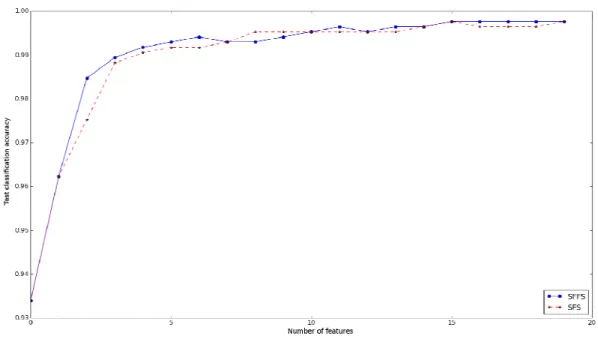
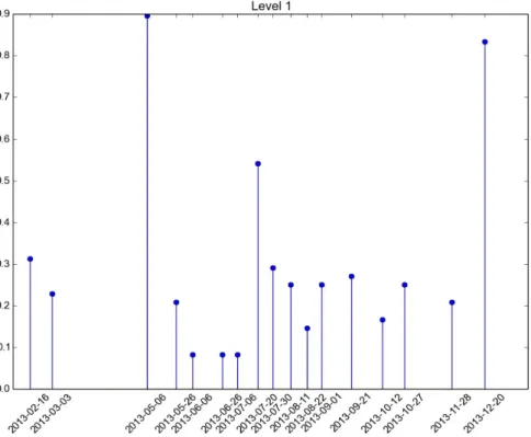
Figure 1.1. Basic principle of NDVI. The healthy vegetation absorbs more Red light (left) than the unhealthy vegetation (right). Source: http://earthobservatory.nasa.gov. ...3 Figure 3.1 Map of France with highlighted study area and typical landscape for study area .19 Figure 3.2. Reference pixels distributed over the study area. Aerial photograph (left) and zoomed part of the reference pixels (right)...20 Figure 3.3. Multispectral image and cloud mask acquired on 12/01/2012...22 Figure 3.4. Forest/non-forest map for the Haute-Garonne department and for the study area (zoomed part). Area covered by forest is presented in green colour. ...23 Figure 4.1 Simplified flow-chart of the project ...24 Figure 4.2. Simplified flow-chart of the pre-processing part of the project ...25 Figure 5.1. Generalized and Ordinary Cross-Validation errors for different values of λ for year 2013...29 Figure 5.2. Temporal profiles of the pixel in blue band before and after smoothing in case without clouds or cloud shadows detected. The temporal profiles are superimposed...30 Figure 5.3. Temporal profiles of the pixel in blue band affected by cloud before and after smoothing (left) and temporal profiles of the pixel in infra-red band affected by cloud shadow before and after smoothing (right) ...30 Figure 5.4. Temporal profiles of the pixel containing NDVI values before and after smoothing affected by clouds ...31 Figure 5.5. Temporal profiles of the pixel in red band before and after smoothing affected by clouds present on two dates ...31 Figure 5.6. The grey-scale images with the clouds present in top-right corner before (left) and after (right) smoothing ...32 Figure 5.7. Test classification accuracy for the different size of feature subsets selected using SFS or SFFS algorithms. Classification was based on the spectral bands together with the NDVI indices for level 2 of classification ...34 Figure 5.8. The most frequently selected dates over 50 repetitions obtained using NPFS classifier for level 1 and year 2013. The selection rate is 1 when the image is selected systematically (50/50)...40 Figure 5.9. The most frequently selected dates over 50 repetitions obtained using NPFS classifier for level 2 and year 2013. The selection rate is 1 when the image is selected systematically (50/50)...41
systematically (50/50)...41 Figure 5.11. Classification maps for level 1 based on spectral bands with GMM (left) and SVM (right)...43 Figure 5.12. Classification maps for level 2 based on spectral bands with GMM (left) and SVM (right)...43 Figure 5.13. Classification maps for level 3 based on spectral bands with GMM (left) and SVM (right)...43 Figure 5.14. Frequency maps obtained for years 2011, 2012, 2013 and 2014 for level 1 based on spectral bands with GMM (left) and SVM (right) ...44 Figure 5.15. Frequency maps obtained for years 2011, 2012, 2013 and 2014 for level 2 based on spectral bands with GMM (left) and SVM (right) ...44 Figure 5.16. Frequency maps obtained for years 2011, 2012, 2013 and 2014 for level 3 based on spectral bands with GMM (left) and SVM (right) ...44 Figure A1.1. The test classification accuracy for Hekla data set (top left), KSC (top right) and Pavia (bottom left) ...48 Figure A1.2. Learning time needed to extract 15 best features for each iteration for Hekla data set (top left), KSC (top right) and Pavia (bottom left) ...49 Figure A3.1. Histograms for Generalized and Ordinary Cross-Validation errors for different values of λ for year 2011...71 Figure A3.2. Histograms for Generalized and Ordinary Cross-Validation errors for different values of λ for year 2012...71 Figure A3.3. Histograms for Generalized and Ordinary Cross-Validation errors for different values of λ for year 2014...71 Figure A3.4. The most frequently selected dates over 50 repetitions obtained using NPFS classifier for level 1 and year 2011. The selection rate is 1 when the image is selected systematically (50/50)...84 Figure A3.5. The most frequently selected dates over 50 repetitions obtained using NPFS classifier for level 2 and year 2011. The selection rate is 1 when the image is selected systematically (50/50)...84 Figure A3.6. The most frequently selected dates over 50 repetitions obtained using NPFS classifier for level 3 and year 2011. The selection rate is 1 when the image is selected systematically (50/50)...85
Figure A3.8. The most frequently selected dates over 50 repetitions obtained using NPFS classifier for level 2 and year 2012. The selection rate is 1 when the image is selected systematically (50/50)...86 Figure A3.9. The most frequently selected dates over 50 repetitions obtained using NPFS classifier for level 3 and year 2012. The selection rate is 1 when the image is selected systematically (50/50)...86 Figure A3.10. The most frequently selected dates over 50 repetitions obtained using NPFS classifier for level 1 and year 2014. The selection rate is 1 when the image is selected systematically (50/50)...87 Figure A3.11. The most frequently selected dates over 50 repetitions obtained using NPFS classifier for level 2 and year 2014. The selection rate is 1 when the image is selected systematically (50/50)...87 Figure A3.12. The most frequently selected dates over 50 repetitions obtained using NPFS classifier for level 3 and year 2014. The selection rate is 1 when the image is selected systematically (50/50)...88 Figure A4.1. The influence of the regularization parameter on smoothing of the simulated data with a second-order penalty (d=2) for several values of the parameter λ ...89 Figure A4.2. Generalized and Ordinary Cross-Validation errors for different values of λ ...90 Figure A4.3 Smoothing the simulated data with
λ
GCV (on the left) andλ
OCV(on the right) ...90Table 3.1. The number of the reference pixels for 14 tree species analyzed in the study ...20 Table 3.2. Characteristics of the Formosat-2 satellite sensor (Site Airbus Defence and Space) ...21 Table 3.3. Meaning of the bits in the mask of clouds and cloud shadows...21 Table 3.4. Formosat-2 imagery, available dates and number of acquired images for each year ...22 Table 5.1 Overall accuracy and Kappa statistics for three defined levels of classification using NDVI indices, spectral bands (SB) and NDVI indices and spectral bands together for year 2013. NPFS_sfs denotes NPFS GMM based classifier computed with a set of features that was chosen using standard feature selection algorithm described in Section 2.3.1. Similarly, NPFS_sffs denotes NPFS GMM based classifier computed with a set of features chosen using SFFS algorithm described in Section 2.3.2. The results correspond to the mean value and variance of the overall accuracy (OA) and Kappa statistics over 50 repetitions in percentages. The best results for each level are reported in bold face...33 Table 5.2 Overall accuracy and Kappa statistics for three defined levels of classification for each of the four years. Only spectral bands were used as the spectral features. NPFS_sfs denotes NPFS GMM based classifier computed with a set of features that was chosen using standard feature selection algorithm described in Section 2.3.1. The results correspond to the mean value and variance of the overall accuracy (OA) and Kappa statistics over 50 repetitions in percentages. The best results for each level were reported in bold face...35 Table 5.3. Confusion matrix for level 1, year 2013. Classification was based on spectral bands and GMM classifier. The results are computed and averaged over 50 repetitions and presented in percentages. ...36 Table 5.4. Confusion matrix for level 1, year 2013. Classification was based on spectral bands and SVM classifier. The results are computed and averaged over 50 repetitions and presented in percentages. ...37 Table 5.5. Confusion matrix for level 2, year 2013. Classification was based on spectral bands and GMM classifier. The results are computed and averaged over 50 repetitions and presented in percentages ...37 Table 5.6. Confusion matrix for level 2, year 2013. Classification was based on spectral bands and SVM classifier. The results are computed and averaged over 50 repetitions and presented in percentages. ...37 Table 5.7. Confusion matrix for level 3, year 2013. Classification was based on spectral bands and GMM classifier. The results are computed and averaged over 50 repetitions and presented in percentages. The main confusion for each species is reported in pink colour. ...38
Table A1.1. Mean values of the overall accuracies and Kappa statistics for each data set ....48 Table A1.2 The mean processing time for learning and prediction for each data set...49 Table A3.1. Overall accuracy and Kappa statistics for three defined levels of classification using NDVI indices, spectral bands (SB) and NDVI indices and spectral bands together for the year 2011. NPFS_sfs denotes NPFS GMM based classifier computed with a set of features that were chosen using standard feature selection algorithm described in Section 2.3.1. Similarly, NPFS_sffs denotes NPFS GMM based classifier computed with a set of features chosen using SFFS algorithm described in Section 2.3.2. The results correspond to the mean value and variance of the overall accuracy (OA) and Kappa statistics over the 50 repetitions in percentages. The best results for each level are reported in bold face...72 Table A3.2. Overall accuracy and Kappa statistics for three defined levels of classification using NDVI indices, spectral bands (SB) and NDVI indices and spectral bands together for the year 2012. NPFS_sfs denotes NPFS GMM based classifier computed with a set of features that were chosen using standard feature selection algorithm described in Section 2.3.1. Similarly, NPFS_sffs denotes NPFS GMM based classifier computed with a set of features chosen using SFFS algorithm described in Section 2.3.2. The results correspond to the mean value and variance of the overall accuracy (OA) and Kappa statistics over the 50 repetitions in percentages. The best results for each level are reported in bold face...73 Table A3.3. Overall accuracy and Kappa statistics for three defined levels of classification using NDVI indices, spectral bands (SB) and NDVI indices and spectral bands together for the year 2014. NPFS_sfs denotes NPFS GMM based classifier computed with a set of features that were chosen using standard feature selection algorithm described in Section 2.3.1. Similarly, NPFS_sffs denotes NPFS GMM based classifier computed with a set of features chosen using SFFS algorithm described in Section 2.3.2. The results correspond to the mean value and variance of the overall accuracy (OA) and Kappa statistics over the 50 repetitions in percentages. The best results for each level are reported in bold face...74 Table A3.4. Confusion matrix for level 1, year 2011. Classification was based on spectral bands and GMM classifier. The results are computed and averaged over 50 repetitions and presented in percentages. ...75 Table A3.5. Confusion matrix for level 1, year 2011. Classification was based on spectral bands and SVM classifier. The results are computed and averaged over 50 repetitions and presented in percentages. ...75 Table A3.6. Confusion matrix for level 2, year 2011. Classification was based on spectral bands and GMM classifier. The results are computed and averaged over 50 repetitions and presented in percentages ...75 Table A3.7. Confusion matrix for level 2, year 2011. Classification was based on spectral bands and SVM classifier. The results are computed and averaged over 50 repetitions and
presented in percentages. The main confusion for each species is reported in pink colour. ...76 Table A3.9. Confusion matrix for level 3, year 2011. Classification was based on spectral bands and SVM classifier. The results are computed and averaged over 50 repetitions and presented in percentages. The main confusion for each species is reported in pink colour. ...77 Table A3.10. Confusion matrix for level 1, year 2012. Classification was based on spectral bands and GMM classifier. The results are computed and averaged over 50 repetitions and presented in percentages. ...78 Table A3.11. Confusion matrix level 1, year 2012. Classification was based on spectral bands and SVM classifier. The results are computed and averaged over 50 repetitions and presented in percentages...78 Table A3.12. Confusion matrix for level 2, year 2012. Classification was based on spectral bands and GMM classifier. The results are computed and averaged over 50 repetitions and presented in percentages ...78 Table A3.13. Confusion matrix for level 2, year 2012. Classification was based on spectral bands and SVM classifier. The results are computed and averaged over 50 repetitions and presented in percentages. ...78 Table A3.14. Confusion matrix for level 3, year 2012. Classification was based on spectral bands and GMM classifier. The results are computed and averaged over 50 repetitions and presented in percentages. The main confusion for each species is reported in pink colour. ...79 Table A3.15. Confusion matrix for level 3, year 2012. Classification was based on spectral bands and SVM classifier. The results are computed and averaged over 50 repetitions and presented in percentages. The main confusion for each species is reported in pink colour. ...80 Table A3.16. Confusion matrix for level 1, year 2014. Classification was based on spectral bands and GMM classifier. The results are computed and averaged over 50 repetitions and presented in percentages. ...81 Table A3.17. Confusion matrix for level 1, year 2014. Classification was based on spectral bands and SVM classifier. The results are computed and averaged over 50 repetitions and presented in percentages. ...81 Table A3.18. Confusion matrix for level 2, year 2014. Classification was based on spectral bands and GMM classifier. The results are computed and averaged over 50 repetitions and presented in percentages ...81 Table A3.19. Confusion matrix for level 2, year 2014. Classification was based on spectral bands and SVM classifier. The results are computed and averaged over 50 repetitions and presented in percentages. ...81
Table A3.21. Confusion matrix for level 3, year 2014. Classification was based on spectral bands and SVM classifier. The results are computed and averaged over 50 repetitions and presented in percentages. The main confusion for each species is reported in pink colour. ...83
Acknowledgment Abstract List of figures List of tables 1 Introduction...1 1.1 General introduction ...1
1.2 Remote sensing and forest ...1
1.3 Working laboratory and study objectives ...3
2 Theoretical background ...6
2.1 Background of smoothing filter ...6
2.1.1 Whittaker smoother for equally spaced data ... 6
2.1.2 Whittaker smoother for unequally spaced data ... 9
2.1.3 Choosing a value for smoothing parameter
λ
... 112.2 Background of feature selection ...13
2.2.1 Non Linear Parsimonious Feature Selection (NPFS)... 13
2.2.2 The Sequential Forward Floating Selection algorithm (SFFS) ... 17
3 Study area and data collection...19
3.1 Study area...19
3.2 Field data collection...19
3.3 Remote sensing data ...21
3.4 Ancillary data...23
4 Methodology ...24
4.1 General procedure ...24
5 Results and discussion ...29
5.1 Pre-processing...29
5.2 Classification...32
6 Conclusion and future work ...45
Appendix 1...47
Appendix 2...51
Appendix 3...71
Appendix 4...89
1 Introduction
1.1 General introduction
Forest is one of dominant terrestrial ecosystem types, providing essential services to the human society, e.g. wood production, climate control, habitat for animal and plant species, carbon sink, water, human recreation [1]. Since the total area under forests is vast, around 4 billion hectares or 31% of the total land area [2], assessment of the forests current and future states is very important.
To correctly estimate the forest state in one area it is necessary to first produce distribution map of the tree species in the study area. Traditionally, distributions of the species were estimated by ground based surveys during forest inventories. However, it is usually better to have tree species distribution maps already during the planning phases of the forest inventory in order to allocate resources and train ground based crews in time. Ground survey is still by far the most accurate and detailed way of forest monitoring, although it is very elaborate, time consuming, and expensive. One of the possible alternatives for consistent and continuous monitoring is to use remote sensing and automated image analysis techniques [3]. Therefore, remote sensing approach for mapping tree species has been researched for a very long time [4]. Nevertheless, accurate estimation of the tree species distributions from remote sensing data is still a very difficult problem, since there are many factors influencing spectral response of species, e.g. tree age, vegetation phase, tree vitality, presence or absence of the understory.
1.2 Remote sensing and forest
Remote sensing is a scientific discipline which analyses and interprets measurements of electromagnetic radiation (EMR) that is reflected from or omitted by a target and observed or recorded from a vantage point by an observer or instrument that is not in contact with the target. Remote sensing can be active or passive, depending on whether the acquired signal was transmitted from a natural source like the sun or it was emitted from an artificial source such as sensors. It is often used for earth observation, which is done by interpreting and understanding EMR measurements of objects on the Earth’s land, ocean or ice surfaces and which are usually made by satellite, together with making relationships between these measurements and the nature of phenomena on the Earth’s surface [5].
Several satellite sensors were launched to collect useful data from Earth's surface in the last decades. Satellite sensors have different spatial, spectral and temporal resolution depending on their function and orbit. The spatial resolution defines the minimum size of an object that can be detected in an image, which determines the pixel size of the images covering the Earth surface. The spectral resolution defines the ability of a satellite to distinguish between two neighbouring wavelengths. Therefore, it depends on the number of spectral bands of the image. Depending on the number of spectral bands, three types of images can be defined: panchromatic (one black-and-white band), multi-spectral images (approximately 3 to 7 bands), and hyper-spectral images (over 100 bands). The higher the spectral resolution is, the higher will be the precision of the spectral signature of an object and it is likely that it will be well discriminated. The temporal resolution is the ability of a satellite sensor to revisit the same area after certain period of time. The temporal resolution is one of the most important
characteristics of the satellites for remote sensing environmental applications. In fact, it is necessary to monitor Earth’s surface changes or short time varying phenomena, caused mainly by human factors or natural evolution of vegetation. Furthermore, the number of acquisitions that could be exploited may be really small because of the bad weather conditions e.g. clouds or cloud shadows, which limit the view of the Earth's surface. Therefore, this can be the reason for not obtaining even one usable image over, for example, several months of acquisition time if the satellite has very low revisiting frequency.
In the past, many attempts to discriminate the tree species were based on the spatial resolution of the data. Tree species classification was performed using aerial photography [6] or high spatial resolution imagery [7], [8]. However, the results showed a limited success with potentially high confusion rates [9]. With only few spectral bands in the multispectral images accuracy of the species discrimination is diminished. Therefore, several studies explored the ability of hyperspectral imagery to identify the tree species. Using LiDAR data or a combination of multiple sources [10], [11], much higher accuracies were obtained, but due to the limited availability and high cost of the hyperspectral imagery, the operational use of these data remains difficult. Thus, several studies have addressed the problem of tree species classification using satellite image time series (SITS). These studies were based on the assumption that phenological variations from the start of the growing season to the senescence should increase the spectral separability of the deciduous tree species [12], due to the dependence of vegetation multispectral reflectance on it’s phenological phases. However, most of the studies looking into SITS potential were based on Landsat time series composed of a limited number of acquisition dates, sometimes from different years, and with only partial coverage of the key phenological periods. Only few studies demonstrated the potential of dense SITS acquired through entire growing season, but all of them were based on airborne images [13], [14].
Currently, it is possible to obtain large dataset with very high temporal resolution using MODIS. However, the spatial resolution of these images is relatively small: 250m (and even 500m or 1km), which is not enough to discriminate different tree species. Until this year the only satellite that could provide SITS with high spatial resolution is FORMOSAT-2. Main issue with this source is the high cost, which is the main reason for relatively few studies using FORMOSAT-2 images. In the future, there is a potential to use Sentinel-2 images to obtain SITS with high spatial resolution. This satellite will provide a global coverage of the Earth's land surface with high spatial resolution optical imagery and high temporal resolution (every 10 days with one satellite and 5 days with 2 satellites) and it will be free of charge. The red band (600 nm to 700 nm) and the near-infrared band (700 nm to 1100 nm) are the most commonly used to characterize the vegetation. From these bands, it is possible to create different indices of vegetation, or to estimate biophysical variables.
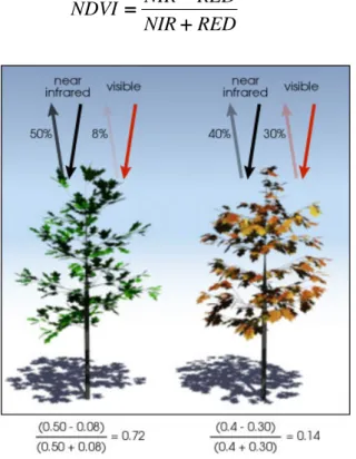
Although there are several vegetation indices, one of the most widely used is the Normalized Difference Vegetation Index (NDVI) [15]. Advantages of the NDVI for monitoring various phenology phases of the vegetation during and between the seasons is that NDVI is very well correlated with the photosynthetic activity and chlorophyll contents, can be easily computed, and it is mostly independent from soil type and current climate conditions. Calculation of the NDVI is based on two properties of the leaf cells of the green plants: 1) chlorophyll pigment
reflecting most of the green, and 2) leaf cell structures reflect around 50% of the near-infrared light (700-1100 nm) that hits them (Figure 1.1). Therefore, presence of the plants is indicated by the reflection of near-infrared light, while plant vitality, if there are any plants present, is indicted by visible light absorption.
NDVI is calculated from the visible (red) and near-infrared light reflected by vegetation using following equation: RED NIR RED NIR NDVI + + + + − − − − = == = (1.1)
Figure 1.1. Basic principle of NDVI. The healthy vegetation absorbs more Red light (left) than the unhealthy vegetation (right). Source: http://earthobservatory.nasa.gov.
From the following NDVI values vary from -1 to 1. Since the reflection in near-infrared band for green vegetation is always higher than in the red band, NDVI values for the vegetation are always higher than 0. Bare ground and water have very low reflectance in the near-infrared band and thus their NDVI values are lower or equal to 0.1. NDVI values from the interval [0.2 – 0.5] indicate the presence of sparse vegetation of grassland and shrubs. NDVI values higher than 0.5 indicate the presence of green leaves (values close to 1 are related to the high density of green leaves) [16]. Finally, it should be noted that NDVI is mostly stable for the conifer species, while it can vary for the broadleaf species.
1.3 Working laboratory and study objectives
My internship was done within the Joint Research Unit DYNAFOR, that is attached to the French National Institute for Agricultural Research (INRA). This public institute was established in 1946. and it is under the joint authority of the Ministries of Research and Agriculture. INRA is composed of 13 departments in order to complete all tasks that are entrusted to it.
DYNAFOR is a JMU (Joint Research Unit) which was established in 2003. Its mission is mainly part of the 6th research area of the INRA center of Toulouse. This unit brings together researchers from two INRA departments: SAD (Science pour l’Action et le Développement) and EFPA (Ecologie des Forêts, Prairies et milieux Aquatiques) with teaching-researchers from ENSAT (Ecole Nationale Supérieure Agronomique de Toulouse) integrated into the National Polytechnic Institute of Toulouse, and teaching-researchers from the EI Purpan (Ecole d’Ingénieurs de Purpan). DYNAFOR activities are focused on the sustainable management of forest resources and rural areas as part of landscape ecology. The main objective of DYNAFOR is to understand and model the relationships between ecological processes, biotechnical processes and socio-economic processes in the management of renewable natural resources. It addresses the current issues in rural and forest areas, induced by global changes that are affected together by the climate, the land use, the biodiversity and the human activities. Finally, another purpose of this JMU is to develop ecological engineering of rural areas so that they could ensure their sustainability and capacity for providing the products and services that are expected by the company.
The organization of DYNAFOR is divided into three main areas: • Area 1: ecosystem services in landscape,
• Area 2: data, space, geomatics and modelling,
• Area 3: biodiversity of rural forests and natural environments.
My work was mainly based on Area 2, with an objective to discriminate tree species from the multi-spectral satellite image time series (SITS) collected in the time period of four consecutive years (2011, 2012, 2013, 2014). In fact in this study the ability of mapping forest species using a dense high resolution multispectral Formosat-2 image time-series was explored. A couple of supervised classification methods were performed and compared in order to find the most convenient method for tree species discrimination. Feature selection algorithm was used to extract the most important features from SITS which represent the best dates for the tree species discrimination. Finally, the thematic maps were produced over the study area for each of the processing years. Thematic maps from different years were then compared to find the most accurate classified species and to assess the robustness of the classifications. This work was initiated by work [17]. It was assumed that phenological variations increase the spectral separability of the deciduous tree species. However, several parts from [17] needed to be improved. Thus, the main tasks of my work were to:
I. Apply smoothing filter to SITS in order to reconstruct pixels contaminated with clouds and cloud shadows in the time series data. In the previous work [17], images that were affected by clouds or cloud shadows were not used for SITS creation. However, since the tree species discrimination was based on the assumption that phenological variations increase the spectral separability of the deciduous tree species it was very important to use all of the available images. Some of the images, affected by bad weather conditions and thus not used in the previous work [17], were acquired during key growing and senescing periods of the year, which may have limited discrimination potential of the study [17]. Therefore, it was expected that adding these images, after smoothing filter application, could significantly improve the identification of the most informative dates for the image acquisition.
II. Perform three supervised classification methods on smoothed SITS created for four years. Instead of using only NDVI indices as the spectral features, and in order to see if it is possible to get a better solution, classification was performed on SITS created from all of the spectral bands and from both NDVI indices and spectral bands together.
III. Implement a new algorithm for feature selection, the Sequential Floating Forward Selection (SFFS), in order to improve the standard feature selection algorithm which was used in the study [17], the Sequential Forward Selection (SFS) algorithm.
IV. Produce thematic maps for each year and compare the results in order to draw conclusions about the robustness of the applied classification methods and to find the spatial distribution of the tree species, which were the most frequently assigned to the same class for the consecutive years.
During the internship period, I had interactions with a Master student Marc Lang and a PhD student Mailys Lopez, who worked in the same laboratory on the grassland classification using the same SITS.
2 Theoretical background
This chapter presents a detailed description of the algorithms used for the purposes of this work.
2.1 Background of smoothing filter
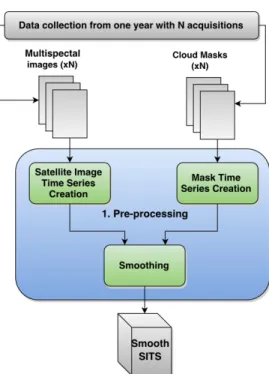
High reliability of the analysed image time series is required for all applications, i.e. the image time series has to be closely related to the observed land surfaces [18]. However, this is not often the case since optical image time series are usually affected by clouds and cloud shadows which add noise to the recorded signal [19]. Therefore, the SITS needs to be smoothed in order to fill data gaps which appeared due to this noise.
In this study, the smoothing of the image time series was performed by Whittaker smoother algorithm [20]. This algorithm is chosen because, compared to other smoothing filters, e.g. [21], it gives continuous control over the smoothness, adapts automatically to the boundaries, deals well with missing values by introducing the vector containing 0 and 1 weights and gives automatic choice for the smoothing parameter due to the fast cross-validation.
Basic Whittaker smoother algorithm, which assumes equally spaced data, is described in Section 2.1.1. Section 2.1.2 describes how basic algorithm can be modified to be applicable on unequally spaced data. The algorithm for selecting the optimal regularization parameter is presented in Section 2.1.3.
2.1.1 Whittaker smoother for equally spaced data
The following notations are used in Section 2.1. Each recorded pixel time series is denoted as N-dimensional vector N
R
z∈ , where N is the number of the time samples:
= ) ( ) (1 N t z t z M z (2.1.1)
Suppose this pixel is contaminated with noise. We can represent each noisy pixel sample as z(ti) = x(ti) + b(ti), where i∈
[
1,...,N]
, x(ti) is a pixel sample we want to retrieve from the noisy sample z(ti) and b is a white noise. Therefore our goal is to find the smooth pixel vector x:
=
)
(
)
(
1 Nt
x
t
x
M
x
(2.1.2)The basic Whittaker smoother algorithm
To describe the basics of the Whittaker smoother we need to assume equally spaced data. Whittaker smoother is based on penalized least squares method with basic principle that smoothing of the noisy/incomplete time series is a compromise between 1) fidelity to the data and 2) roughness of the reconstruction. Whittaker smoother finds the smooth series x that minimizes a function combining these two conflicting goals.
The measure of the roughness Rd can be expressed as a squared sum of the differences i d x ∆ , where i d x
∆ represents a d order difference of xi:
∑
= ∆ = N i i d d x R 1 2 ) ( (2.1.3)The 1st order difference is: 1 − − = ∆xi xi xi (2.1.4)
General expression for dth order difference is: ) ( 1 i d i d x x =∆ ∆ − ∆ . (2.1.5)
For example the 2nd and 3rd order differences are:
2 1 2 1 1 2 2 ) ( ) ( ) (∆ = − − − − − − = − − + − ∆ = ∆ xi xi xi xi xi xi xi xi xi (2.1.6) 3 2 1 3 2 1 2 1 2 3 3 3 ) 2 ( ) 2 ( ) (∆ = − − + − − − − − + − = − − + − − − ∆ = ∆xi xi xi xi xi xi xi xi xi xi xi xi (2.1.7) Deviation of the smooth pixel x from the observed pixel z can be expressed as the sum of the squared differences between observed samples zi and smooth samples xi:
2 1 ) (
∑
= − = N i i i x z S (2.1.8)The function which combines these two measures is:
d R S
Q==== ++++
λ
(2.1.9)Parameter λ in equation (2.1.9) is a smoothing parameter that has to be defined by the user. With increasing parameter λ, influence of the roughness in x will be stronger and the deviation of x from the observation z will also increase. Some examples showing this effect are given in Appendix 4. The aim of the penalized least squares is to find series x that minimizes the final function Q.
Q==== z−−−−x ++++λ Ddx ====(z−−−−x) (z−−−−x)++++λx Dd Ddx (2.1.10)
In equation (2.1.10) =
∑
iai2 2
a is a quadratic norm of any vector a and Ddis a matrix such that Ddx====Δdx. E.g. for the first order difference and N=6, matrix D1 is a
(
N − 1)
×N givenby: − − − − − = 1 1 0 0 0 0 0 1 1 0 0 0 0 0 1 1 0 0 0 0 0 1 1 0 0 0 0 0 1 1 1 D (2.1.11)
Finding partial derivatives of the final function Q and equating them to 0, we get the solution for the pixel vector x:
z D D I x x D D x z x 1 ) ( 0 2 ) ( 2 − − − − + + + + = = = = ⇒ ⇒ ⇒ ⇒ = = = = + + + + − − − − − − − − = = = = ∂ ∂∂ ∂ ∂ ∂∂ ∂ d T d d T d Q
λ
λ
(2.1.12)In equation (2.1.12) I is N×Nidentity matrix.
Dealing with missing data
The previous algorithm for smoothing can be easily modified to smooth the observations with missing values. In this case the vector of weights w is introduced of the length equal to the length of z (in our case N). Vector w can take values wi=0 for missing data elements and
1 = i
w for non-missing data elements. With missing values in the data, deviation of the smooth pixel x from the observed pixel z is changed to:
∑
= − − = − = N i T i i i z x w S 1 2 ) ( ) ( ) ( z x W z x (2.1.13)Where W is N×Nmatrix with vector w on its diagonal.
The measure of the roughness Rd is calculated in the same way as in equation (2.1.3).
The final function Q changes to:
x D D x x z W x z T d d T T Q====( −−−− ) ( −−−− )++++
λ
(2.1.14)In the same way as in equation (2.1.12) a solution for the smooth pixel x is calculated as: Wz D D W x x D D x z W x 1 ) ( 0 2 ) ( 2 − + = ⇒ = + − − = ∂ ∂ d T d d T d Q
λ
λ
(2.1.15)2.1.2 Whittaker smoother for unequally spaced data
It is often necessary to adapt basic Whittaker smoother algorithm to the algorithm for smoothing unequally spaced data since the period between two consecutive image acquisitions is usually not constant.
Deviation of the smooth pixel from the observed pixel (S) is estimated as for the equally spaced data with missing values (equation 2.1.13).
The measure of the roughness of x, Rd , is given as:
2 1 )) ( (
∑
= ∆ = N i i d d x t R = D x xTDdTDdx d ==== 2 (2.1.16)The equation (2.1.16) looks the same as the equation (2.1.3) but for unequally spaced data the difference will change and therefore the measure of the roughness will also change e.g. for d=1, the difference and the measure of the roughness for unequally spaced data will be:
2 2 1 1 1 1 1) ( ) ( ) ( ) ( ) (
∑
∑
∑
∑
= == = −−−− − − − − − − − − − − − − − − − − − − − − = = = = ⇒ ⇒ ⇒ ⇒ − −− − − −− − = = = = N i i i i i i i i i i t t t x t x R t t t x t x t x ∆ (2.1.17)Thus, matrix D1 is given as:
− − − = − − − = N N N N t t t t t t t t t t t t δ δ δ δ δ δ δ δ δ δ δ δ 1 1 0 0 0 1 1 0 0 0 1 1 1 1 0 0 0 1 1 0 0 0 1 1 1 1 0 0 0 1 1 0 0 0 1 1 3 3 2 2 3 3 2 2 1 L M O O O M L L L M O O O M L L L M O O O M L L D (2.1.18)
where δti =ti−ti−1. Size of the matrix D1 is (N− )1 ×N.
The second order difference is:
2 1 2 ( ) ( ) ) ( − − − ∆ − ∆ = ∆ i i i i i t t t x t x t x (2.1.19)
1 2 2 1 1 2 4 4 2 3 4 3 4 2 3 3 2 2 3 2 3 2 2 ) )( ( 1 ) )( ( 1 ) )( ( 1 0 0 0 ) )( ( 1 ) )( ( 1 ) )( ( 1 0 0 0 ) )( ( 1 ) )( ( 1 ) )( ( 1 D Δ D ==== − − − − − − − − − − − − = == = − − − − − − − − N N N N N N t t t t t t t t t t t t t t t t t t δ δ δ δ δ δ δ δ δ δ δ δ δ δ δ δ δ δ L M O M L L (2.1.20)
where δ2ti = ti - ti-2 and Δ2 is:
− − − − − − − − − − − − = == = N N t t t t t t 2 2 4 2 4 2 3 2 3 2 2 1 1 0 0 0 1 1 0 0 0 1 1 δ δ δ δ δ δ L M O M L L Δ (2.1.21)
And finally, a dth order difference is:
d i i i d i d i d t t t x t x t x − − − − − ∆ − ∆ = ∆ ( ) ( ) ( 1) 1 1 (2.1.22)
To find matrix Dd the following recursion is used:
1 − − − − = = = = d d d Δ D D (2.1.23) with − − − − − −− − = == = + + + + + + + + N d N d d d d d d t t t t δ δ δ δ 1 1 0 0 0 0 1 1 1 1 L M O M L Δ (2.1.24)
where δdti = ti - ti-d .
Thus, the derivative matrix of order d is obtained using the recursive formula:
1 2 1...Δ D Δ Δ Dd ==== d d−−−− (2.1.25)
Replacing deviation of the smooth from the observed pixel and roughness in the function Q and finding partial derivatives (see equation 2.1.12) a solution for the smooth pixel x is obtained as: Wz D D W x d 1 ) ( ++++ −−−− = == = T d
λ
(2.1.26)2.1.3 Choosing a value for smoothing parameter λ
Value for the smoothing parameter λ can be iteratively chosen until we obtain a visually satisfactory result. However, more objective and automatic choice for λ can be made using cross-validation [20].
The procedure is done by leaving out one of the non-missing elements of the pixel time series zi for i∈
{
1, ..., N}
, then applying Whittaker smoother to the remaining elements andpredicting the left out element. Cross-validation error is found by doing this procedure for all non-missing elements of the pixel z. Regularization parameter is chosen so that prediction is as good as possible, i.e. error of the prediction is minimum.
Ordinary Cross-Validation
The Ordinary Cross-Validation mean square error is defined as:
(
)
∑
∑
= − − = N i i i i i i i w t x t z w OCV 1 2 ) ) ( ( 1 ) (λ
(2.1.27) In equation (2.1.27), i i tx( )− is the estimation of the value z(ti) after removing the th
i element of z.
For the chosen interval for λ, the Ordinary Cross-Validation Estimate of λ is: ) ( min arg λ λ λ OCV R OCV + ∈ = (2.1.28)
Using the equation (2.1.26) and introducing the hat matrix H follows: Hz x W D D W H = = = = ⇒ ⇒⇒ ⇒ + + + + = = = = −−−−1 ) ( d T d
λ
(2.1.29){
1,...,N}
i for , ) ( ) ( 1 ∈ =∑
= j j ij i h z t t x (2.1.30)After removing the ithelement of the vector z, estimation x ti i
− ) ( is: ii i ii i i i i i ii i ii i i i i i ii j N j N i j j ij j ij i i i i i j j N j j ij i i h t z h t x t x t x h t z h t x t x t x h t z h t z h t x t x i j if t x i j if t z t x where t x h t x − − − − − − − − = = = = ⇒ ⇒ ⇒ ⇒ − − − − = = = = − − − − ⇒ ⇒ ⇒ ⇒ − −− − − − − − = = = = − − − − ⇒ ⇒⇒ ⇒ = = = = ≠ ≠≠ ≠ = == = = = = = − −− − − − − − − − − − − − − − = == = ≠ ≠ ≠ ≠ = = = = − − − − − − − − = = = = − −− −
∑
∑
∑
∑
∑
∑
∑
∑
∑
∑
∑
∑
1 ) ( ) ( ) ( ) ( ) ( ) ( ) ( ) ( ) ( ) ( ) ( ) ( , ) ( , ) ( ) ( ) ( ) ( 1 1 1 (2.1.31) Replacing i i tx( )− in equation (2.1.27), OCV of the parameter λ is:
∑
∑
= − − = N i i ii i i i i w h t x t z w OCV 1 2 1 ) ( ) ( 1 ) (λ
(2.1.32) Generalized Cross-ValidationTo compute Generalized Cross-Validation error, hii is replaced by the mean of the diagonal elements of the matrix H:
[
]
[
]
2 1 2 2 1 2 ) ( 1 ) ( ) ( 1 ) ( 1 ) ( ) ( 1 ) ( − − = − − =∑
∑
∑
∑
∑
∑
= = i i N i i i i i i i i N i i i i i i w H trace w t x t z w H I trace w w t x t z w GCV λ (2.1.33)As for Ordinary Cross-Validation, for chosen interval of the parameter λ, the Generalized Cross-Validation Estimate of λ is selected as:
) ( min arg λ λ λ GCV R GCV + ∈ = (2.1.34)
2.2 Background of feature selection
Image classification is used for producing the thematic maps which provide an informative description of the study area, i.e. the thematic maps show spatial distribution of the tree species inside area of interest. Furthermore, classification was used in this project for selecting the best features, which in this case represent the most useful images to discriminate tree species and better define the image acquisition plan.
In this study, discrimination of the tree species from the multi-temporal images was performed with three supervised learning methods: Support Vector Machines (SVM) [22, Chapter 12], Random Forest (RF) [22, Chapter 15] and Gaussian Mixture Model (GMM) classifier. Nonlinear Parsimonious Feature Selection (NPFS) package was used to learn GMM model. NPFS was presented in [23] and represents feature selection algorithm which is used in this study for indentifying the most important dates for discriminating the tree species.
The basics of the NPFS algorithm are described in Section 2.2.1. Section 2.2.2 presents the Sequential Floating Forward Selection (SFFS) algorithm as the replacement for the standard feature selection algorithm in the NPFS.
2.2.1 Non Linear Parsimonious Feature Selection (NPFS)
Nonlinear Parsimonious Feature Selection (NPFS), compiles a pool of selected features by iteratively selecting a spectral feature from the original set of features. This pool is used to learn a Gaussian Mixture Model (GMM). Successive features will be selected according to their classification rate, until the stopping criterion is reached. The estimation of the classification rate is done using k-fold Cross-Validation (k-CV).
Fast GMM parameterization when k-CV is computed is crucial for the efficient implementation of the NPFS. From the following, it is possible to quickly perform k-CV and forward selection by using parameter update rules and the marginalization properties of the Gaussian distribution.
Gaussian Mixture Model
Let S == x==
{{{{
((((
i,yi))))
}}}}
in====1 be a set of training pixels, where xi is a D-dimensional pixel vector,D i∈∈∈∈R
x and yi∈
{
1,...,C}
its class. C is the number of classes, n is the number of training pixels and nc is the number of training pixels belonging to the class c.A Gaussian mixture model is a probabilistic model, which assumes that each pixel vector is generated from a mixture of a finite number of the Gaussian distributions as:
∑
= = C c cp c p 1 ) / ( ) (x π x (2.2.1)In equation (2.2.1)
π
c is a prior probability for each class (0≤π
c ≤1 and 1 1 =∑
= c cπ
) and p(x/c) is a prior class conditional probability function for pixel vector x given as a D-dimensional Gaussian distribution: − − − − − − − − − − − − = == = 1/2
∑
∑
∑
∑
−−−−1 2 / 2( ) ( ) 1 exp ) 2 ( 1 ) / ( c c T c c D c p x μ x μ Σ xπ
(2.2.2)where μc is the mean vector of the class c and, Σc and Σc are the covariance matrix of the class c and its determinant.
According to Bayes rule, the posterior probability of the class c when given the pixel vector x is: ) ( ) / ( ) / ( x x x p c p c p =
π
c (2.2.3)Using the maximum a posteriori rule, pixel vector is classified to the class c if
[
C]
j j p c p( /x)≥ ( /x),∀ ∈1,... .Since in equation (2.2.3) p(x) is a constant which does not affect the final result, the maximum a posteriori rule is given by:
Assign x to class c if arg max ( / ) ,..., 1 p j c j C j=
π
x = (2.2.4)After replacing the eq. (2.2.2) in eq. (2.2.4) and by taking the log of eq. (2.2.4) the final decision rule is given as:
) ln( 2 ) ln( ) ( ) ( ) ( c1 c c c T c c Q x ====−−−− x−−−−μ
∑
∑
∑
∑
−−−− x−−−−μ −−−− Σ ++++π
(2.2.5) The estimators of the model parameters are obtained using standard maximization of the log-likelihood as: T c i c i n i c c n i i c c c c c c n n n n ) )( ( 1 , 1 , 1 1 ∧ ∧ ∧ ∧ ∧ ∧ ∧ ∧ = == = ∧ ∧ ∧ ∧ = = = = ∧ ∧ ∧ ∧ ∧ ∧ ∧ ∧ − −− − − − − − = = = = = = = = = = = =∑
∑
∑
∑
∑
∑
∑
∑
μ x μ x Σ x μπ
(2.2.6)The Sequential Forward Feature Selection (SFS)
The main goal of feature selection is to select a subset of k features from the given set of D measurements, k<D, without significantly degrading the performance of the recognition system [24]. Feature selection techniques usually need a criterion for evaluating a performance of the model and an optimization procedure for finding the subset of features that maximizes/minimizes the criterion [25].
Let Xk =
{
xi:1≤i≤k,xi∈Y}
be the set of k features selected from the complete set of measurements Y ===={{{{
yi:1≤≤≤≤i≤≤≤≤ D}}}}
, where D is the number of available features.The basic Sequential Forward Selection (SFS) method can be split in several steps [22, Chapter 3] [26]:
• Start with an empty set of selected features, Xk = Ø
• Iteratively add the most significant feature with respect to Xk from the set of available features Y- Xk
• Stop if the increase of the estimated classification rate is too low or if the maximum number of the features is reached
Classification rate was estimated with stratified k-fold cross-validation. The set of training pixels S was divided into k subsets of equal size. Each subset contains approximately the same percentage of the pixels which belong to the same class as the initial set S. One of the k-subsets was used for model testing, while remaining k-subsets were used as a training data. Since each of the k subsets needs to be used exactly once for validation, this procedure was repeated exactly k times. The k test errors were computed and then averaged to compute the mean test error.
Fast estimation of the GMM sub-models parameters during the Cross-validation process
Suppose the number of the pixels used for validation during the Cross Validation procedure is v. Parameters of the model Sn-v can be estimated from the full learned GMM model using update rules. Classification rate can be estimated with subset of features using marginalization properties of the Gaussian distribution parameters. Therefore, GMM model needs to be learned only once during the entire training step.
The update rules after removing v samples for validation: Rule 1 (Class proportion):
v n v n c n c v n c − − = ∧ − ∧
π
π
(2.2.7) In equation (2.2.7) cn ∧ π and cn v − ∧π are the proportions of the class c computed over n and (n-v) samples, respectively and vcis the number of the removed pixels which belong to the class
c. Note that
∑
= = C c c v v 1 .Rule 2 (Mean vector): c c v c c n c c v n c v n v n c c c c − −− − − −− − = = = = ∧ ∧∧ ∧ ∧ ∧ ∧ ∧ − − − − ∧ ∧ ∧ ∧ μ μ μ (2.2.8) In equation (2.2.8) c n c ∧ ∧ ∧ ∧ μ and c c v n c − − − − ∧ ∧∧ ∧
μ are the mean vectors of the class c computed over nc and nc - vc training samples and
c v c ∧ ∧∧ ∧
μ is the mean vector of the class c computed over vc removed samples.
Rule 3 (Covariance matrix):
T v c n c v c n c c c c c v c c c c n c c c c v n c c c c c c c c c v n v n v n v v n n ) )( ( ) ( ) ( ) ( 2 ∧ ∧ ∧ ∧ ∧ ∧∧ ∧ ∧ ∧ ∧ ∧ ∧ ∧∧ ∧ − − − − − − − − − − − − − − − − − − − − − − − − − − − − − − − − = == = Σ Σ μ μ μ μ Σ (2.2.9) In equation (2.2.9), nc c Σ and nc vc c − −− −
Σ are the covariance matrices of the class c computed over nc and nc - vc training samples, respectively.
Marginalization of Gaussian distribution
To get the GMM model over a subset of the original feature set, it is only necessary to exclude non-selected features from the mean vector and the covariance matrix [27].
If initial set of features is represented as: x=
[
xs,xns]
, where xs and xns are selected and non-selected feature sets, respectively, then mean vector and covariance matrix computed over the full model can be written as:] , [μs μns μ==== ∧ ∧ ∧ ∧ (2.2.10) = == = ns ns s ns ns s s s , , , , Σ Σ Σ Σ Σ (2.2.11)
From the marginalization of Gaussian distribution follows that xs is also a Gaussian distribution with mean vector μs and covariance matrix Σs,s. Therefore, when full model is learned, all of the sub-models built with a subset of the original variables will be available at no additional computational cost.
2.2.2 The Sequential Forward Floating Selection algorithm (SFFS)
Sequential forward selection algorithm (SFS), described in Section 2.2.1, suffers from the so-called "nesting effect", which means that features once selected can not be excluded later from the pool of the selected features. This can lead to the sub-optimal subset of the chosen features. Since there is rather widely accepted belief [24, 29, 30, 31] that floating search methods (Sequential Forward Floating Selection (SFFS) and Sequential Backward Floating Selection (SBFS)) [24] are superior to the simple sequential ones, SFS and SBF [28], SFFS algorithm [24][32, Chapter 9] is implemented in this study as a modification of the original SFS algorithm in order to avoid its “nesting effect”.
If the k features have already been selected and form the subset Xk with its criterion function J(Xk), the values of the criterion function J(Xi) have to be stored for all the previously subsets
of size i =1,2,...(k-1). As in the SFS algorithm, in this project, J represents the estimated classification rate.
The SFFS algorithm also starts from the empty set of features (k=0 and X0=Ø). For the selection of the first two features original SFS method is applied. Then the algorithm continues with the step 1.
• Step 1: Inclusion. Using the basic SFS method, select the most significant feature xk+1 with respect to Xk from the set of available measurements, Y- Xk, and add it to the subset Xk. The most significant feature is obtained as:
[
( ( )]
max arg ) ( 1 J X x x k X Y x k k + = − ∈ + (2.2.12)Thus the new formed feature set is Xk+1 = Xk+ xk+1. • Step 2: Conditional exclusion.
Find the least significant feature in the set Xk+1 as:
[
( ( )]
max arg 1 1 x X J x k X x r k − = + ∈ + (2.2.13) 1. If the least significant feature is the one just added in the first step, xr = xk+1,keep it, set the number of selected features to k=k+1 and return to step 1. 2. If xr is the least significant feature and 1≤r≤k, exclude it from the set Xk+1 to
form the new subset X'k = Xk+1 - xr. Note that now J(X'k) > J(Xk). If k=2 set Xk= X'k, J(Xk ) = J(X'k) and return to step 1, otherwise continue with the step 3.
• Step 3: Continuation of conditional exclusion.
In the same way as in the Step 2, find the least significant feature xs in the set X'k . 1. If J(X'k - xs) ≤ J(Xk-1) set Xk= X'k, J(Xk )=J(X'k ) and return to Step 1.
2. If J(X'k - xs) > J(Xk-1) then exclude xsfrom X'k to form new set X'k-1 = X'k - xs. Set k=k-1. If k=2 set Xk= X'k , J(Xk )=J(X'k ) and return to step 1, otherwise repeat Step 3.
3 Study area and data collection
3.1 Study area
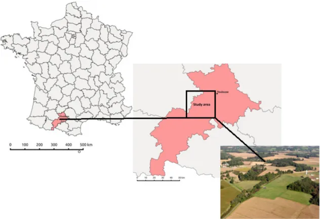
The study area is located in southwest of France, in Midi-Pyrénées region, about 30 km west of Toulouse (Figure 3.1). Climate of the area is characterized by mild and rainy winters and dry and hot summers, i.e. Cfb climate type as classified by Köppen-Geiger climate classification system [33]. Annual mean air temperature is higher than 13°C while mean annual precipitation is 656 mm. Forests are found on 10 % of the area, while the most prevalent tree species is Oak (Quercus spp.). Non-forest part of the area consists of grasslands and crops (combination of wheat, sunflower and maize).
Figure 3.1 Map of France with highlighted study area and typical landscape for study area
3.2 Field data collection
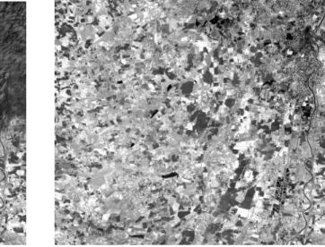
Since supervised classification methods were used for tree species discrimination, it was necessary to use ground truth data, which was collected by the DYNAFOR lab. during three surveys in November 2013, January 2014 and May 2014. In total, 1038 sample points of the dominant broadleaf and conifer tree species were collected from the study area. Two observers were used to record each plot covering approximately an area of 576 m2, which is equivalent to nine contiguous FORMOSAT-2 pixels of 8m x 8m. Each plot was homogeneous in terms of tree species. GPS coordinates of plots were estimated with Garmin GPSMap 62st receiver and all the plots were distributed over the whole study area. Plots were later converted to polygons of one pixel size to use them in the classification (Figure 3.2).
Three thematic levels based on the Forest National Inventory [34] were defined from the collected ground truth data (Table 3.1). The first one classifies the forest into broadleaf and coniferous species (level 1). The second level splits level 1 forest groups into two sub-categories. Broadleaf forests are for the most part deciduous, except for the evergreen Eucalyptus, while conifer forests can be pine forest or other. Finally, third level includes all the fourteen tree species. Sample size per species varied from 35 pixels for Black locust and Douglas fir to 209 pixels for Aspen.
Level 1 Level 2 Level 3 Sample size
Broadleaf Broadleaf Broadleaf Broadleaf Broadleaf Broadleaf Broadleaf Broadleaf Deciduous Deciduous Deciduous Deciduous Deciduous Deciduous Deciduous Evergreen
Silver birch (Betula pendula)
Pedunculate/Pubescent/Sessile oak (Quercus robur/pubescens/petraea) Red oak (Quercus rubra)
European ash (Fraxinus excelsior) Aspen (Populus tremula)
Black locust (Robinia pseudoacacia) Willow (Salix) Eucalyptus (Eucalyptus) 75 125 100 40 209 35 39 100 Conifer Conifer Conifer Conifer Conifer Conifer Pine Pine Pine Pine Other conifer Other conifer
Corsican pine (Pinus nigra subsp. laricio) Maritime pine (Pinus pinaster)
Black pine (Pinus nigra subsp. salzmannii) Austrian black pine(Pinus nigra var. austriaca) Douglas fir (Pseudotsuga menziesii)
Silver fir (Abies alba)
40 40 40 85 35 75
Table 3.1. The number of the reference pixels for 14 tree species analyzed in the study
Figure 3.2. Reference pixels distributed over the study area. Aerial photograph (left) and zoomed part of the reference pixels (right).