HAL Id: hal-00326650
https://hal.archives-ouvertes.fr/hal-00326650v2
Submitted on 13 Jan 2010
HAL is a multi-disciplinary open access
archive for the deposit and dissemination of
sci-entific research documents, whether they are
pub-lished or not. The documents may come from
teaching and research institutions in France or
abroad, or from public or private research centers.
L’archive ouverte pluridisciplinaire HAL, est
destinée au dépôt et à la diffusion de documents
scientifiques de niveau recherche, publiés ou non,
émanant des établissements d’enseignement et de
recherche français ou étrangers, des laboratoires
publics ou privés.
A posteriori error estimates including algebraic error:
computable upper bounds and stopping criteria for
iterative solvers
Pavel Jiranek, Zdenek Strakos, Martin Vohralík
To cite this version:
Pavel Jiranek, Zdenek Strakos, Martin Vohralík. A posteriori error estimates including algebraic
error: computable upper bounds and stopping criteria for iterative solvers. SIAM Journal on
Sci-entific Computing, Society for Industrial and Applied Mathematics, 2010, 32 (3), pp.1567-1590.
�10.1137/08073706X�. �hal-00326650v2�
ERROR AND STOPPING CRITERIA FOR ITERATIVE SOLVERS
PAVEL JIR ´ANEK∗, ZDENˇEK STRAKOˇS†, AND MARTIN VOHRAL´IK‡
Abstract. For the finite volume discretization of a second-order elliptic model problem, we derive a posteriori error estimates which take into account an inexact solution of the associated linear algebraic system. We show that the algebraic error can be bounded by constructing an equilibrated Raviart–Thomas–N´ed´elec discrete vector field whose divergence is given by a proper weighting of the residual vector. Next, claiming that the discretization error and the algebraic one should be in balance, we construct stopping criteria for iterative algebraic solvers. An attention is paid, in particular, to the conjugate gradient method which minimizes the energy norm of the algebraic error. Using this convenient balance, we also prove the efficiency of our a posteriori estimates, i.e., we show that they also represent a lower bound, up to a generic constant, for the overall energy error. A local version of this result is also stated. This makes our approach suitable for adaptive mesh refinement which also takes into account the algebraic error. Numerical experiments illustrate the proposed estimates and construction of efficient stopping criteria for algebraic iterative solvers.
Key words.Second-order elliptic partial differential equation, finite volume method, a posteriori error estimates, iterative methods for linear algebraic systems, conjugate gradient method, stopping criteria.
AMS subject classifications. 65N15, 65N30, 76M12, 65N22, 65F10
1. Introduction. In numerical solution of partial differential equations, the
computed result is an approximate solution found in some finite-dimensional space. A natural question is whether this solution is a sufficiently accurate approximation of the exact (weak) solution of the problem at hand. A posteriori error estimates aim at giving an answer to this question while providing upper bounds on the dif-ference between the approximate and exact solutions that can be easily computed. Their mathematical theory for the finite element method was started by the pioneer-ing paper by Babuˇska and Rheinboldt [7] and a vast amount of literature on this
subject exists nowadays; we refer, e.g., to the books by Verf¨urth [48] or Ainsworth
and Oden [2]. For the cell-centered finite volume method, Ohlberger [31] derives a posteriori estimates for the convection–diffusion–reaction case, whereas, for the pure diffusion case, Achdou et al. [1] use the equivalence of the discrete forms of the schemes with some finite element ones, Nicaise [30] gives estimates for Morley-type interpolants of the original piecewise constant finite volume approximation, and Kim [23] devel-ops a framework applicable to any locally conservative method. Recently, general guaranteed a posteriori estimates for locally conservative methods have been derived in [50, 51, 52].
∗Faculty of Mechatronics and Interdisciplinary Engineering Studies, Technical University of Liberec, H´alkova 6, 46117 Liberec, Czech Republic & CERFACS, 42 Avenue Gaspard Coriolis, 31100 Toulouse, France ([email protected]). The work of this author was supported by the grant No. 201/09/P464 of the GACR and by the project IAA100300802 of the GAAS.
†Institute of Computer Science, Academy of Sciences of the Czech Republic, Pod Vod´arenskou vˇeˇz´ı 2, 18207 Prague, Czech Republic ([email protected]). The work of this author was supported by the project IAA100300802 of the GAAS and by the Institutional Research Plan AV0Z10300504 “Computer Science for the Information Society: Models, Algorithms, Applications.”
‡UPMC Univ. Paris 06, UMR 7598, Laboratoire Jacques-Louis Lions, 75005 Paris,
France & CNRS, UMR 7598, Laboratoire Jacques-Louis Lions, 75005 Paris, France
([email protected]). The work of this author was supported by the GNR MoMaS project “Numerical Simulations and Mathematical Modeling of Underground Nuclear Waste Disposal”, PACEN/CNRS, ANDRA, BRGM, CEA, EdF, IRSN, France.
Apart from few exceptions, existing a posteriori estimates rely on the assumption that the linear system resulting from discretization is solved exactly. This is not as-sumed, e.g., in the work by Wohlmuth and Hoppe [53], but the bounds are valid only
for a sufficiently refined mesh, and/or contain various unspecified constants. R¨ude
[38, 39, 40] gives estimates of the energy norm of the error based on the norms of the residual functionals obtained from some particular stable splitting of the underlying Hilbert space. Repin [35] or Repin and Smolianski [36] do not use any information about the discretization method and the method for solving the resulting linear alge-braic system. This makes the estimates very general but the price is that they may be rather costly and not sufficiently accurate.
A moderately sized system of linear algebraic equations can be solved by a direct method. For large systems, preconditioned iterative methods, see, e.g., Saad [41], be-come competitive, and with increasing size they represent the only viable alternative. It should, however, be emphasized that applications of direct and iterative methods are principally different. While in direct methods the whole solution process must be completed to the very end in order to get a meaningful numerical solution, iterative methods can produce an approximation of the solution at each iteration step. The amount of computational work depends on the number of iterations performed, and an efficient PDE solver should use this principal advantage by stopping the algebraic solver whenever the algebraic error drops to the level at which it does not significantly affect the whole error (cf. [6, 46]). The simplest, most often used, and mathematically most questionable stopping criterion is based on evaluation of the relative Euclidean norm of the residual vector, see, e.g., the discussion in [22, Section 17.5]. There is only a rough connection of the algebraic residual norm with the size of the whole error in approximation of the continuous problem (we discuss this point in detail in Section 7.1 below) and, usually, not even this connection is considered. Consequently, one either continues the algebraic iterations until the residual norm is not further reduced (i.e., one uses the iterative solver essentially as a direct solver, possibly wasting resources and computational time without getting any further improvement of the whole error), or stops earlier at a risk that the computed solution is not sufficiently accurate. For some enlightening comments we refer, e.g., to [32].
The question of stopping criteria has been addressed, e.g., by Becker et al. [10] with emphasize on the multigrid solver, see also [9] and the recent paper [25]. A remarkable early approach relating the algebraic and discretization errors is repre-sented by the so-called cascadic conjugate gradient method of Deuflhard [16], which was further studied by several other authors, see, e.g., [42]. In [3], Arioli compares the bound on the discretization error with the error of the iterative method when solving self-adjoint second-order elliptic problems. He uses the relationship between the energy norm defined in the underlying Hilbert space for the weak formulation and its restriction onto the discrete space, in combination with the numerically stable algebraic error bounds [45], see also [46]. Arioli et al. [5] extend these results for non self-adjoint problems. Their approach is interesting and useful in some applications but relies on an a priori knowledge, not an a posteriori bound for the discretization error. It is also worth to point out the recent results on stopping criteria for Krylov subspace methods in the framework of mixed finite element methods applied to linear and nonlinear elliptic problems [4]. Stopping the algebraic iterative solver based on a priori information on the discretization error is also applied in the context of wavelet discretizations of elliptic partial differential equations by Burstedde and Kunoth [13]. Finally, the interesting technique of Patera and Rønquist [32], see also Maday and
Patera [24], gives computable lower and upper asymptotic bounds of a linear func-tional of an approximate linear system solution. If the asymptotics is attained for a reasonable number of iterations, this allows to construct a stopping criterion. Such criterion is, however, tailored to a fast converging preconditioned primal-dual conju-gate gradient Lanczos method, and, at least in the presented form, it does not relate the discretization and algebraic parts of the error.
In this paper we consider a second-order elliptic pure diffusion model problem: find a real-valued function p defined on Ω such that
−∇ · (S∇p) = f in Ω, p = g on Γ := ∂Ω, (1.1)
where Ω is a polygonal/polyhedral domain (open, bounded, and connected set) in Rd,
d = 2, 3, S is a diffusion tensor, f is a source term, and g prescribes the Dirichlet boundary condition. Details are given in Section 2. For the discretization of prob-lem (1.1) on simplicial meshes, we consider in Section 3 a general locally conservative cell-centered finite volume scheme, cf. Eymard et al. [17].
The first goal of this paper is to derive a posteriori error estimates which take into account an inexact solution of the associated linear algebraic system. Section 5 extends for this purpose the a posteriori error estimates from [50, 51]. The derived upper bound consists of three estimators: an estimator measuring the nonconfor-mity of the approximate solution, which essentially reflects the discretization error; an estimator corresponding to the interpolation error in the approximation of the source term f which in general turns out to be a higher-order term; and an abstract algebraic error estimator corresponding to the inexact solution of the discrete
lin-ear algebraic problem, based on equilibrated vector fields rh from the lowest-order
Raviart–Thomas–N´ed´elec space whose divergences are given by a proper weighting of the algebraic residual vector.
The second goal of this paper is to construct, in the context of solving prob-lem (1.1), efficient stopping criteria for iterative algebraic solvers. Our approach is based on comparison of the discretization and algebraic error estimates, see Section 6. Under the assumption of a convenient balance between the two estimates we also prove the (local) efficiency of our estimates. They can thus correctly predict the over-all error size and distribution and are suitable for adaptive mesh refinement which takes into account the inaccuracy of the algebraic computations.
Section 7 gives fully computable upper bounds or estimates for the abstract al-gebraic error estimator of Section 5. The first upper bound is given directly by the components of the algebraic residual vector. The second approach is based on the estimates for the algebraic error measured in the energy norm, for which there exist efficient estimates, namely in the conjugate gradient method. The last approach is
based on a factual construction of a vector field rh and on the use of its
comple-mentary energy kS−1
2rhk as the algebraic error estimator. All three approaches are numerically illustrated in Section 8 on several examples.
2. Notation, assumptions, and the continuous problem. Our notation is
standard, see [15, 12, 17], and it is included here for completeness. It can be skipped and used as a reference, if needed, while reading the rest of the paper.
Recall that Ω is a polygonal domain in R2or a polyhedral domain in R3with the
boundary Γ. Let Th be a partition of Ω into closed simplices, i.e., triangles if d = 2
and tetrahedra if d = 3, such that Ω = ∪K∈ThK. Moreover, we assume that the
partition is conforming in the sense that if K, L ∈ Th, K 6= L, then K ∩ L is either
by EK the set of sides (edges if d = 2, faces if d = 3) of K, by Eh= ∪K∈ThEK the set
of all sides of Th, and by Eint
h and Ehext, respectively, the interior and exterior sides.
We also use the notation EK for the set of all σ ∈ Eint
h which share at least a vertex
with a K ∈ Th. For interior sides such that σ = σK,L:= ∂K ∩ ∂L, i.e., σK,Lis a part
of the boundary ∂K and, at the same time, a part of the boundary ∂L, we shall call
K and L neighbors. We denote the set of neighbors of a given element K ∈ Th by
TK; TK stands for all triangles sharing at least a vertex with K ∈ Th. For K ∈ Th,
nwill always denote its exterior normal vector; we shall also employ the notation nσ
for a normal vector of a side σ ∈ Eh, whose orientation is chosen arbitrarily but fixed
for interior sides and coinciding with the exterior normal of Ω for exterior sides. For
σK,L ∈ Eint
h such that nσ points from K to L and a sufficiently smooth function ϕ
we also define the jump operator [[·]] by [[ϕ]] := (ϕ|K)|σ− (ϕ|L)|σ. Finally, a family
of meshes T := {Th; h > 0} is parameterized by h := maxK∈ThhK, where hK is the
diameter of K (we also denote by hσ the diameter of σ ∈ Eh).
For a given domain S ⊂ Rd, let L2(S) be the space of square-integrable (in
the Lebesgue sense) functions over S, (·, ·)S the L2(S) inner product, and k · kS
the associated norm (we omit the index S when S = Ω). By |S| we denote the Lebesgue measure of S and by |σ| the (d − 1)-dimensional Lebesgue measure of a
(d − 1)-dimensional surface σ in Rd. Let H(S) be a set of real-valued functions
defined on S. By [H(S)]d we denote the set of vector functions with d components
each belonging to H(S). Let next H1(S) be the Sobolev space with square-integrable
weak derivatives up to order one, H1
0(S) ⊂ H1(S) its subspace of functions with traces
vanishing on Γ, H1/2(S) the trace space, H(div, S) := {v ∈ [L2(S)]d; ∇ · v ∈ L2(S)}
the space of functions with square-integrable weak divergences, and let finally h·, ·i∂S
stand for (d − 1)-dimensional L2(∂S)-inner product on ∂S. We also let H1
Γ(Ω) :=
{ϕ ∈ H1(Ω); ϕ|
Γ = g} be the set of functions satisfying the Dirichlet boundary
condition on Γ in the sense of traces. For a given partition Th of Ω, let H1(Th) :=
{ϕ ∈ L2(Ω); ϕ|K ∈ H1(K) ∀K ∈ Th} be the broken Sobolev space. Finally, we let
W (Th) be the space of functions with mean values of the traces continuous across
interior sides, i.e., W (Th) := {ϕ ∈ H1(Th); h[[ϕ]], 1iσ = 0 ∀σ ∈ Eint
h }, and W0(Th) its
subspace with mean values of traces over boundary sides equal to zero, W0(Th) :=
{ϕ ∈ W (Th); hϕ, 1iσ= 0 ∀σ ∈ Eext
h }.
We next denote by Pk(S) the space of polynomials on S of total degree less
than or equal to k and by Pk(Th) := {ϕh ∈ L2(Ω); ϕh|K ∈ Pk(K) ∀K ∈ Th} the
space of piecewise k-degree polynomials on Th. We define RTN(K) := [P0(K)]d+
xP0(K) for an element K ∈ Th the local and RTN(Th) := {vh ∈ [L2(Ω)]d; vh|K ∈
RTN(K) ∀K ∈ Th} ∩ H(div, Ω) the global lowest-order Raviart–Thomas–N´ed´elec
space of specific piecewise linear vector functions. Recall that the normal components
of vh ∈ RTN(K), vh · n, are constant on each σ ∈ EK and that they represent
the degrees of freedom of RTN(K). By consequence, the constraint vh ∈ H(div, Ω)
imposing the normal continuity of the traces is expressed as vh|K · n + vh|L· n = 0
for all σK,L ∈ Eint
h and there is one degree of freedom per side in RTN(Th). Recall
also that ∇ · vh is constant for vh∈ RTN(K). For more details, we refer to Brezzi
and Fortin [12] or Quarteroni and Valli [33].
Assumption 2.1 (Data). Let S be a symmetric, bounded, and uniformly positive
definite tensor, piecewise constant on Th. Let in particular cS,K > 0 and CS,K > 0
denote its smallest and largest eigenvalues on each K ∈ Th. In addition, let f ∈ Pl(Th)
be an elementwise l-degree polynomial function and g ∈ H1/2(Γ).
satisfied in practice. Otherwise, interpolation can be used in order to get the desired
properties. In the sequel, we will employ the notation SK := S|K, and, in general,
ϕK:= ϕh|K for ϕh∈ P0(Th).
We define a bilinear form B by
B(p, ϕ) := X
K∈Th
(S∇p, ∇ϕ)K, p, ϕ ∈ H1(Th)
and the corresponding energy (semi-)norm by
|||ϕ|||2:= B(ϕ, ϕ). (2.1)
Note that ||| · ||| becomes a norm on the space W0(Th), cf. [49]. Also note that B
is well-defined for functions from the space H1(Ω) as well as from the broken space
H1(Th). The weak formulation of problem (1.1) is then to find p ∈ H1
Γ(Ω) such that
B(p, ϕ) = (f, ϕ) ∀ϕ ∈ H01(Ω). (2.2)
Assumption 2.1 implies that problem (2.2) admits a unique solution [15].
3. Finite volume methods and postprocessing. We start with description
of the finite volume methods for problem (1.1). In these methods, the approximation
ph of the solution p in (1.1) is only piecewise constant and it is not appropriate for
an energy a posteriori error estimate, as ∇ph = 0. We therefore construct a locally
postprocessed approximation using information about the known fluxes. Finally, we
will in the a posteriori error estimates need an H1(Ω)-conforming approximation using
the so-called Oswald interpolate.
3.1. Finite volume methods. A general cell-centered finite volume method
for problem (1.1) (cf., e.g., [17]) can be written as: find ph∈ P0(Th) such that
X σ∈EK
UK,σ= fK|K| ∀K ∈ Th, (3.1)
where fK := (f, 1)K/|K| and UK,σ is the diffusive flux through the side σ of an
element K, depending linearly on the values of ph, so that (3.1) represents a system of linear algebraic equations of the form
SP = H, (3.2)
where S ∈ RN ×N and P, H ∈ RN with N being the number of elements in the
partition Th. Here we only assume the continuity of the fluxes, i.e., UK,σ = −UL,σ
for all σ = σK,L∈ Eint
h , so that practically all finite volume schemes can be included.
We next give an example which clarifies the ideas.
Let there be a point xK ∈ K for each K ∈ Th such that if σK,L ∈ Ehint, then
xK 6= xL and the straight line connecting xK and xL is orthogonal to σK,L. Let an
analogous orthogonality condition hold also on the boundary. Then Th is admissible
in the sense of [17, Definition 9.1]. Under the additional assumption SK = sKI (I
denotes the identity matrix) on each K ∈ Th, the following choice is possible:
UK,σ= −sK,L|σK,L| dK,L (pL− pK) for σ = σK,L∈ E int h , UK,σ= −sK |σ| dK,σ(gσ− pK) for σ ∈ EK∩ E ext h . (3.3)
Here pK are the cell values of ph(pK:= ph|Kfor all K ∈ Th) and the value of sK,Lon
a side σ = σK,L∈ Eint
h is given by sK,L= ωσ,KsK+ωσ,LsL, where ωσ,K = ωσ,L =12 in
the case of the arithmetic averaging and ωσ,K = sL/(sK+sL) and ωσ,L = sK/(sK+sL)
in the case of the harmonic averaging of the diffusion coefficients sK. The symbol
dK,L stands for the Euclidean distance between the points xK and xL and dK,σ for
the distance between xK and σ ∈ EK ∩ Eext
h . Finally, gσ := hg, 1iσ/|σ| is the mean
value of g on a side σ ∈ Eext
h . To express (3.1), (3.3) in the matrix form (3.2), let
the elements of Th be enumerated using a bijection ℓ : Th → {1, . . . , N}. With the
corresponding ordering of the unknown values pK of ph defined by (P )ℓ(K) = pK
for each K ∈ Th, and denoting respectively by (·)kl and (·)k the matrix and vector
components, the system matrix S and the right-hand side vector H are all zero except the elements defined by
(S)ℓ(K),ℓ(K)= X
L∈TK
sK,L|σK,L|
dK,L +
X σ∈EK∩Ehext
sK |σ|
dK,σ,
(S)ℓ(K),ℓ(L)= −sK,L|σK,L|
dK,L , L ∈ TK,
(H)ℓ(K)= fK|K| + X
σ∈EK∩Ehext
sK |σ|
dK,σgσ.
The system matrix S is therefore symmetric and positive definite and, moreover, irreducibly diagonally dominant (for the definition of this term, see, e.g., [47]).
3.2. Postprocessing. Let uh∈ RTN(Th) be prescribed by the fluxes UK,σ, i.e.,
for each K ∈ Thand σ ∈ EK, let uh be such that
(uh|K· n)|σ:= UK,σ/|σ|. (3.4)
We define a postprocessed approximation ˜ph∈ P2(Th) in the following way:
−SK∇˜ph|K= uh|K, ∀K ∈ Th, (3.5a)
(1 − µK)(˜ph, 1)K/|K| + µKph(xK) = pK,˜ ∀K ∈ Th. (3.5b)
Here µK = 0 or 1, depending on whether in the particular finite volume scheme (3.1)
pK represents the approximate mean value of ph on K ∈ Th or the approximate
point value in xK, respectively. It is not difficult to show that such ˜ph exists, is
unique, but nonconforming (does not belong to H1(Ω)), see [50, Section 4.1] and [51,
Section 3.2.1]. For the finite volume scheme (3.1), (3.3), ˜ph∈ W (Th) if f = 0, but if
f 6= 0 then ˜ph6∈ W (Th) in general. Under the condition that the finite volume scheme
at hand satisfies some convergence properties it is shown in [51] that ∇˜ph→ ∇p and
˜
ph→ p in the L2(Ω)-norm for h → 0 and that optimal a priori error estimates hold.
Note finally that the described postprocessing is local on each element and its cost is negligible.
3.3. Oswald interpolation operator. For a given function ϕh ∈ Pk(Th), the
Oswald interpolation operator IOsfrom Pk(Th) to Pk(Th)∩H1(Ω) is defined as follows
(cf., e.g., [1]): let x be a Lagrangian node, i.e., a point where the Lagrangian degree of
freedom for Pk(Th) ∩ H1(Ω) is prescribed, see [15, Section 2.2]. If x lies in the interior
Otherwise, the value of IOs(ϕh) at x is defined by the average of the values of ϕh at this node from the neighboring elements, i.e.,
IOs(ϕh)(x) = 1
Nx
X K∈Tx
ϕh|K(x),
where Tx := {K ∈ Th; x ∈ K} is the set of elements of Th containing the node x
and Nxdenotes the number of elements contained in this set. Finally, let IOsΓ (ϕh) be
a modified Oswald interpolate (cf. [51]) differing from IOs(ϕh) only on such K ∈ Th
that contain a boundary side and such that
IOsΓ (ϕh)|Γ = g in the sense of traces.
4. Inexact solution of systems of linear algebraic equations. Let Pa be
an approximate solution of (3.2), i.e., SPa≈ H. We then have the equation
SPa
= H − R, (4.1)
where R := H −SPais the algebraic residual vector associated with the approximation
Pa. This means that an approximate solution Paof problem (3.2) is the exact solution
of the same problem with a perturbed right-hand side Ha := H − R. Defining pa
h ∈ P0(Th) by pa
K := (Pa)ℓ(K) and a residual function ρh ∈ P0(Th) associated with the
algebraic residual vector R by
ρK := (R)ℓ(K)/|K|, K ∈ Th, (4.2)
equation (4.1) is equivalent to the set of conservation equations X
σ∈EK
Ua
K,σ= fK|K| − ρK|K| ∀K ∈ Th. (4.3)
The fluxes UK,σa are of the same form as UK,σ, with the values of ph replaced by pah.
Compared to (3.1), equation (4.3) contains an additional term on the right-hand side representing the error from the inexact solution of the algebraic system. We can
now define ua
h∈ RTN(Th) by (uah|K· n)|σ:= UK,σ/|σ|, so that (4.3) impliesa
huah· n, 1i∂K = fK|K| − ρK|K| ∀K ∈ Th. (4.4)
We can consequently, as in Section 3.2, build a postprocessed approximation ˜pa
h ∈ P2(Th) by
−SK∇˜pah|K= uah|K, ∀K ∈ Th, (4.5a)
(1 − µK)(˜pah, 1)K/|K| + µKp˜ah(xK) = paK, ∀K ∈ Th. (4.5b)
The backward error idea of incorporating the algebraic error into (4.1), together with the construction (4.4) and (4.5), will form a basis for our a posteriori error estimates presented next.
5. A posteriori error estimates including the algebraic error. We first
recall the following result proved as a part of [50, Lemma 7.1] (here ||| · ||| is the energy (semi-)norm defined by (2.1)):
Lemma 5.1 (Abstract a posteriori error estimate). Consider arbitrary p ∈ H1 Γ(Ω) and ˜p ∈ H1(Th). Then |||p − ˜p||| ≤ inf s∈H1 Γ(Ω) |||˜p − s||| + sup ϕ∈H1 0(Ω) |||ϕ|||=1 B(p − ˜p, ϕ).
Before formulating the a posteriori error estimate, we recall the Poincar´e
inequal-ity. It states that for a convex polygon/polyhedron K and ϕ ∈ H1(K),
kϕ − ϕKkK ≤
1
πhKk∇ϕkK, (5.1)
where ϕK := (ϕ, 1)K/|K| is the mean of ϕ over K. Our a posteriori error estimates
are based on the following theorem:
Theorem 5.2 (A posteriori error estimate including the algebraic error). Let p be the weak solution of (1.1) given by (2.2) with the data satisfying Assumption 2.1. Let a
couple pa
h∈ P0(Th), uah∈ RTN(Th) be given, where uah satisfies (4.4) for some given
function ρh ∈ P0(Th). Finally, let ˜pa
h ∈ P2(Th) be the postprocessed approximation
given by (4.5a)–(4.5b). Then
|||p − ˜pah||| ≤ ηNC+ ηO+ ηAE, (5.2)
where the global nonconformity and oscillation estimators are given by
ηNC := ( X K∈Th ηNC,K2 )1 2 and ηO:= ( X K∈Th ηO,K2 )1 2 ,
respectively, and ηAE stands for the algebraic error estimator defined by
ηAE:= inf rh∈RTN(Th) ∇·rh=ρh sup ϕ∈H1 0(Ω) |||ϕ|||=1 (rh, ∇ϕ). (5.3)
The local nonconformity and oscillation estimators are respectively given by ηNC,K:= |||˜pa h− IOsΓ (˜pah)|||K, ηO,K:= 1 π√cS,K hKkf − fKkK, and IΓ
Os(˜pah) is the modified Oswald interpolant of ˜pah described in Section 3.3.
Proof. For any s ∈ H1
Γ(Ω) we have from Lemma 5.1
|||p − ˜pah||| ≤ |||˜pah− s||| + sup ϕ∈H1 0(Ω) |||ϕ|||=1 B(p − ˜pah, ϕ) = |||˜pah− s||| + sup ϕ∈H1 0(Ω) |||ϕ|||=1 [TO(ϕ) + TAE(ϕ)] ≤ |||˜pa h− s||| + sup ϕ∈H1 0(Ω) |||ϕ|||=1 TO(ϕ) + sup ϕ∈H1 0(Ω) |||ϕ|||=1 TAE(ϕ), (5.4) where TO(ϕ) := PK∈Th(S∇(p − ˜p a
h) + rh, ∇ϕ)K and TAE(ϕ) := −(rh, ∇ϕ) for an
The term TO(ϕ) can be expressed using the definition of the weak solution (2.2),
(4.5a), and the Green theorem as (recall that rh, ua
h∈ H(div, Ω) and ϕ ∈ H01(Ω)) TO(ϕ) = (f, ϕ) − X K∈Th (S∇˜pah− rh, ∇ϕ)K = (f, ϕ) + (rh+ uah, ∇ϕ) = (f − ∇ · (rh+ uah), ϕ). (5.5)
Since the divergence is piecewise constant for functions in RTN(Th), the Green the-orem with (4.4) gives for any K ∈ Th
(∇ · uah)|K= (∇ · uah, 1)K/|K| = huah· n, 1i∂K/|K| = fK− ρK. (5.6)
Thus, employing ∇ · rh|K= ρK,
f − ∇ · (rh+ uah) = f − ρK− fK+ ρK = f − fK ∀K ∈ Th.
Now let ϕK := (ϕ, 1)K/|K| be the mean value of ϕ over K. Using the above identities,
we can rewrite (5.5) in the form
TO(ϕ) = X
K∈Th
(f − fK, ϕ − ϕK)K
and from the Cauchy–Schwarz inequality, the Poincar´e inequality (5.1), and using |||ϕ||| = 1, we obtain the estimate
TO(ϕ) ≤ X K∈Th kf − fKkKkϕ − ϕKkK≤ X K∈Th ηO,K|||ϕ|||K ≤ ( X K∈Th ηO,K2 )1 2 . With (5.4), putting s = IΓ
Os(˜pah) and noticing that rh∈ RTN(Th) such that ∇·rh= ρh
was chosen arbitrarily, the proof is finished.
Remark 5.3 (Form of the a posteriori error estimate). By (4.5a) and by defini-tion (2.1) of the energy (semi-)norm, posing u := −S∇p,
|||p − ˜pah||| =°°S−12(u − ua h)
° °,
so that the a posteriori error estimate of Theorem 5.2 equivalently controls the energy norm of the error in the flux.
The a posteriori error estimate given in Theorem 5.2 consists of three parts: the
nonconformity estimator ηNCindicating the departure of the approximate solution ˜pa
h
from the space H1(Ω), the oscillation estimator ηOwhich measures the interpolation
error in the right-hand side of problem (1.1), and the algebraic error estimator ηAE which accounts for the error from the inexact solution of the algebraic system. Note
that the nonconformity estimator depends on the actual approximation ˜pa
hof ˜phand
thus implicitly also on ρh and not only on the discretization error, whereas the
al-gebraic error estimator depends only on the residual function ρh associated with the
algebraic residual vector R, see (4.2). We discuss computable upper bounds on ηAE
in Section 7 below. Finally, whenever f ∈ H1(Th), the oscillation estimator ηO is of
higher order by the Poincar´e inequality (5.1) (it converges as O(h2) for h → 0) and
its value is significant only on coarse grids or for highly varying S. We shall give some more details in the next section.
The following remark follows from the freedom of choice of s and rh in the proof of Theorem 5.2:
Remark 5.4 (Abstract form of Theorem 5.2). With the assumptions of Theo-rem 5.2, |||p − ˜pah||| ≤ ηNCA + ηO+ ηAAE with ηNCA := inf s∈H1 Γ(Ω) |||˜pah− s|||, ηAAE:=r inf ∈H(div,Ω) ∇·r=ρh sup ϕ∈H1 0(Ω) |||ϕ|||=1 (r, ∇ϕ), (5.7)
and ηO as in Theorem 5.2. Please note that
ηANC≤ ηNC and ηAAE≤ ηAE.
We now show that the abstract algebraic error estimator ηA
AEgiven above is equal
to the complementary energy of the flux of the solution of the original problem (1.1) with homogeneous Dirichlet boundary condition and the right-hand side replaced by the residual function ρh.
Theorem 5.5 (Equivalence of the abstract algebraic error estimator and of the
minimal complementary energy). Consider an arbitrary ρh ∈ P0(Th) and ηA
AE given
by (5.7). Then
ηAEA = kS− 1 2qk,
where q ∈ H(div, Ω), ∇·q = ρh, is the unique minimizer of the complementary energy
characterized by
kS−12qk = min
r∈H(div,Ω) ∇·r=ρh
kS−12rk, (5.8)
or, equivalently, by q = −S∇e, where e ∈ H1
0(Ω) is the unique weak solution of
−∇ · (S∇e) = ρh in Ω, e = 0 on Γ. (5.9)
Proof. Using the Cauchy–Schwarz inequality,
ηAEA =r inf ∈H(div,Ω) ∇·r=ρh sup ϕ∈H1 0(Ω) |||ϕ|||=1 (r, ∇ϕ) ≤ sup ϕ∈H1 0(Ω) |||ϕ|||=1 (q, ∇ϕ) = sup ϕ∈H1 0(Ω) |||ϕ|||=1 (S−12q, S 1 2∇ϕ) ≤ sup ϕ∈H1 0(Ω) |||ϕ|||=1 ¡ kS−12qk|||ϕ|||¢= kS− 1 2qk.
Before proceeding to the converse, let us recall that the problem of finding q as the minimizer of the complementary energy is equivalent to the problem of finding
q∈ H(div, Ω), ∇ · q = ρh, such that
see, e.g., [33, Theorem 7.1.1]. Let now r ∈ H(div, Ω) such that ∇·r = ρhbe arbitrary.
Then, by (5.10), it holds (S−1q, q − r) = 0, and using that q = −S∇e, we get
kS−1 2qk2= (S−1q, q) = (S−1q, q − r) + (S−1q, r) = (−∇e, r). Hence kS−1 2qk = |||e||| = µ r,−∇e |||e||| ¶ ≤ sup ϕ∈H1 0(Ω) |||ϕ|||=1 (r, ∇ϕ),
which concludes the proof by virtue of the fact that r ∈ H(div, Ω) such that ∇·r = ρh was chosen arbitrarily.
6. Stopping criterion for iterative solvers and efficiency of the a
poste-riori error estimate. In PDE solvers, the discretization and algebraic errors should
be in balance. This requirement leads to a stopping criterion for iterative algebraic solvers applied to discretized linear algebraic systems. Using this approach, we also prove in this section global and local efficiency of our a posteriori error estimates in the sense that the estimators also represent global and local lower bounds (up to a generic constant) for the error in the energy (semi-)norm. Please note that all the
results presented below still hold when ηAEis replaced by one of its computable upper
bounds presented in Section 7 below.
6.1. Stopping criterion. A stopping criterion that we propose requires the
value of the algebraic error estimator to be related to the nonconformity one via
ηAE≤ γ ηNC, 0 < γ ≤ 1, (6.1)
where γ is typically close to 1. This leads to the bound
|||p − ˜pah||| ≤ (1 + γ)ηNC+ ηO.
Let ηAEcan be constructed using local contributions ηAE,K corresponding to
individ-ual elements K ∈ Th so that
ηAE= ( X K∈Th ηAE,K2 )1 2 . (6.2)
We will use such construction below. Then one can consider also a local stopping criterion of the form
ηAE,K ≤ γKηNC,K, 0 < γK ≤ 1 ∀K ∈ Th, (6.3)
where γK are typically close to 1.
In the rest of this section we will employ the notation cS,TK := minL∈TKcS,L,
which is the lower bound on the eigenvalues of the diffusion tensor S on the patch
of elements TK (see Section 2). The notation C, eC, and C will stand for generic
constants dependent on the quantities specified below, possibly different at different occurrences. We will also make use of the following assumption:
Assumption 6.1 (Shape regularity of T ). There exists a constant θT > 0 such
that minK∈ThhK/̺K ≤ θT for all Th ∈ T , where ̺K is the diameter of the largest
6.2. Efficiency of the estimates. Let us first introduce some additional
nota-tion. For ϕ ∈ H1(Th) and σ = σL,M ∈ Eint
h , put kϕk#,σ := h
−1 2
σ |h[[ϕ]], 1iσ|. Note that
h[[ϕ]], 1iσ= 0 for all σ ∈ Eint
h for ϕ ∈ W (Th), as kϕk#,σ only measures the jump in the
mean values of ϕ. Then, for a given set of sides E, let |||ϕ|||2#,E:= cS,E
X σ∈E
kϕk2#,σ,
where cS,E is the minimum of the values cS,K over all K ∈ Th which have at least
one side in the set E. The following theorem shows that using the local stopping criterion (6.3), the derived estimates also represent local lower bounds for the error. Consequently, they are suitable for adaptive mesh refinement.
Theorem 6.2 (Local efficiency of the a posteriori error estimate). Let the as-sumptions of Theorem 5.2 and Assumption 6.1 be satisfied. Let (6.2) hold together
with (6.3). Then, for each K ∈ Th,
ηNC,K+ ηAE,K ≤ (1 + γK)¡CC 1 2 S,Kc −1 2 S,TK(|||p − ˜p a h|||TK+ |||p − ˜pah|||#,EK) +|||IOs(˜pah) − IOsΓ (˜pah)|||K¢.
If, moreover, the local algebraic error estimators are given by ηAE,K = kS−1
2rhkK for
some rh such that rh∈ RTN(Th), ∇ · rh= ρh, then
ηNC,K+ ηO,K+ ηAE,K ≤ eC(1 + γK)(|||p − ˜pah|||TK+ |||p − ˜pah|||#,EK
+ |||IOs(˜pah) − IOsΓ (˜pah)|||K).
(6.4) Here the constant C depends only on the space dimension d and on the shape
regu-larity parameter θT and eC depends in addition on the polynomial degree l of f (see
Assumption 2.1) and on the ratio CS,K/cS,TK.
Proof. It has been proved in [50, Theorem 4.4], [51, Theorem 4.2], and [52, Theorem 6.15], using the tools from [48] and [1], that for any piecewise polynomial function ˜pa h∈ Pm(Th), ηNC,K≤ C Ã C 1 2 S,Kc −1 2 S,TK|||p − ˜p a h|||TK+ C 1 2 S,K X σ∈EK kp − ˜pahk#,σ ! (6.5a) +|||IOs(˜pah) − IOsΓ (˜pah)|||K, π−1c− 1 2 S,KhKkf + ∇ · (S∇˜p a h)kK ≤ CC 1 2 S,Kc −1 2 S,K|||p − ˜p a h|||K, (6.5b)
where the constant C depends only on d, θT, and the polynomial degree m of ˜pa
h, and
C depends in addition on the polynomial degree l of f .
The first assertion of the theorem is thus an immediate consequence of (6.5a) and
of (6.3). For the second one, we have to bound ηO,K. Using fK = (∇ · uah)|K+ ρK
from (5.6), uah|
K = −SK∇˜pah|K from (4.5a), the triangle inequality, and ∇ · rh= ρh,
we have ηO,K = π−1c− 1 2 S,KhKkf − fKkK ≤ π −1c−1 2 S,KhK(kf + ∇ · (S∇˜p a h)kK+ k∇ · rhkK).
The first term on the right-hand side of this inequality is bounded by (6.5b). Using the inverse inequality (cf. [33, Proposition 6.3.2]) and Assumption 2.1,
k∇ · rhkK ≤ Ch−1K krhkK≤ Ch −1 K C 1 2 S,KkS −1 2rhkK
for some constant C only depending on d and θT. Thus, using (6.3), ηO,K≤ CC 1 2 S,Kc −1 2 S,K|||p − ˜p a h|||K+ CC 1 2 S,Kc −1 2 S,KγKηNC,K.
The assertion (6.4) thus follows by combining the above estimate with the previous ones.
Using the global stopping criterion (6.1) without (6.2) and (6.3), we obtain the
following global lower bound (note that the result for estimators ηNC and ηAE is
standard and sufficient, as the estimator ηO represents only data oscillations and is
generally of higher order; it can also be included as shown in Theorem 6.2):
Theorem 6.3 (Global efficiency of the a posteriori error estimate). Let the assumptions of Theorem 5.2 and Assumption 6.1 be satisfied and let (6.1) hold. Then
ηNC+ ηAE≤ eC(1 + γ)(|||p − ˜pah||| + |||p − ˜pah|||#,Eint
h + |||IOs(˜p
a
h) − IOsΓ (˜pah)|||),
where the constant eC depends only on d, θT, and maxK∈ThCS,K/cS,TK.
Proof. From (6.1), ηNC+ ηAE≤ (1 + γ)ηNC. Using the definition of ηNC,
employ-ing (6.5a) and the inequality (a + b)2≤ 2a2+ 2b2, we have
ηNC+ ηAE≤ (1 + γ)√2 ( X K∈Th ¡ CCS,Kc−1S,TK(|||p − ˜p a h|||2 TK+ |||p − ˜pah|||2#,EK) +|||IOs(˜pah) − IOsΓ (˜pah)|||2K ¢) 1 2 , from where the assertion of the theorem follows.
We remark that the terms |||IOs(˜pah) − IΓ
Os(˜pah)|||K in the above theorems penalize the possible violation of the Dirichlet boundary condition and they can be nonzero
only for boundary simplices. The term |||p − ˜pah|||#,Eint
h = |||˜p
a h|||#,Eint
h then accounts
for the discontinuity of the means of traces of the postprocessed approximation ˜pa
h and for a part of the algebraic error. In our numerical experiments it was negligible. Bound (6.4) is in particular relevant to the cases investigated in Section 7.3 below, where the algebraic error estimator admits the desired form.
7. Computable upper bounds and estimates for the algebraic error
estimator. The algebraic error estimator ηAE of Section 5 was defined in a general
way without specification of the techniques for computing it. In this section we discuss
three different approaches giving computable upper bounds on ηAE or its efficient
estimates.
7.1. Simple bound using the algebraic residual vector. A guaranteed
up-per bound on the algebraic error ηAE can be obtained using a weighted Euclidean
norm of the algebraic residual vector R defined in (4.1). This worst case-like sce-nario approach can lead to large overestimation, cf. Section 8 below; for a supportive algebraic reasoning see, e.g., [22, Section 17.5].
Lemma 7.1 (Algebraic error estimator using the algebraic residual vector). The
algebraic error estimator ηAE from Theorem 5.2 can be bounded as
ηAE≤ η(1)AE:= s CF,Ω cS,Ω hΩ ( X K∈Th ρ2K|K| )1 2 , (7.1)
where cS,Ω:= minK∈ThcS,K and hΩis the diameter of the domain Ω.
Proof. Using the Green theorem and the Cauchy–Schwarz inequality, we have
(rh, ∇ϕ) = −(∇ · rh, ϕ) = − X K∈Th (ρK, ϕ)K≤ ( X K∈Th ρ2K|K| )1 2 kϕk. (7.2)
As ϕ ∈ H0(Ω), we can now relate kϕk to |||ϕ||| using the Friedrichs inequality by1
kϕk ≤pCF,ΩhΩk∇ϕk ≤
s CF,Ω
cS,Ω hΩ|||ϕ||| .
(7.3) Considering |||ϕ||| = 1 and combining (7.2) and (7.3) proves the statement. As for the value of CF,Ω, we refer to, e.g., Neˇcas [29, Section 1.2] or Rektorys [34, Chapter 30];
it ranges between 1/π2and 1. Note that hΩmay be replaced by the infimum over the
thicknesses of Ω in the given direction, cf., e.g., [49].
We point out that (7.1) can be rewritten in the algebraic form as ηAE(1) = s CF,Ω cS,Ω hΩ√RtD−1R = s CF,Ω cS,Ω hΩkRkD−1, (7.4)
where D := diag(|ℓ−1(k)|)Nk=1 is a finite volume-type mass matrix and ℓ represents
the enumeration of elements in Th defined in Section 3.1.
7.2. Estimate based on the energy norm of the algebraic error. Inspired
by Theorem 5.5, consider the approximation of (5.9) by the finite volume scheme given
in Section 3.1. It consists in finding eh∈ P0(Th) such that
X σ∈EK
UK,σ= ρK|K| ∀K ∈ Th, (7.5)
where UK,σ are the prescribed fluxes, which depend linearly on the values of eh. In
matrix form, this leads to
SE = R, (7.6)
where S is the matrix from (3.2). The matrix S is symmetric and positive definite
(SPD), see Section 3.1, so that it induces an algebraic energy norm k · kSby kXk2S:=
XtSX for a vector X ∈ RN. We now shed some light on the relationship between
ηAE and kEkS.
Let us construct a postprocessed error ˜eh ∈ P2(Th) from eh and UK,σ given
by (7.5) as described in Section 3.2 and put qh:= −S∇˜eh. Then qh∈ RTN(Th) and
∇ · qh= ρhby (7.5), so that
ηAE≤ ηAE(2) := kS−
1
2q
hk (7.7)
follows directly from definition (5.3) of ηAE and the Cauchy–Schwarz inequality, see
the proof of Theorem 5.5. Suppose for the moment that ˜eh∈ W0(Th) and that µK= 0
in (3.5b) for all K ∈ Th. Under these conditions and using the Green theorem, ¡ ηAE(2)¢2= kS−12qhk2= X K∈Th (S∇˜eh, ∇˜eh)K = X K∈Th ©
(−∇ · (S∇˜eh), ˜eh)K+ hS∇˜eh|K· n, ˜ehi∂Kª
= X
K∈Th
(−∇ · (S∇˜eh), ˜eh)K = X
K∈Th
Here the term PK∈T
hhS∇˜eh|K· n, ˜ehi∂K vanishes due to the fact that S∇˜eh· n is
sidewise constant as S∇˜eh ∈ RTN(Th) and the assumption ˜eh ∈ W0(Th).
Unfortu-nately, as discussed in Section 3.2, ˜ehin the finite volume method does not in general
belong to the space W0(Th). Numerical experiments however show that the violations of the means of traces continuity are typically very slight. Therefore
ηAE≤ ηAE(2) = kS−
1
2qhk ≈ kEkS, (7.8)
and kEkSsuggest itself as an a posteriori algebraic error estimate. We now switch to
linear algebra considerations of estimating kEkS.
Let a system of the form (3.2) be given and let S be SPD, so the conjugate
gradient method (CG) [21] can be used. Let PCG
n be the CG approximation to the
solution P computed at the iteration step n, Pa= PCG
n , SPnCG= H − RCGn , see (4.1),
ECG
n := P − PnCG, SEnCG= RCGn , see (7.6). Since the original paper [21] it is known
that the Euclidean norm of the residual kRCG
n k does not represent a reliable measure
of the quality of the CG approximation PCG
n . CG minimizes the algebraic energy
norm of the error kECG
n kSover the Krylov subspaces
Kn(S, RCG0 ) := span{RCG0 , SRCG0 , . . . , Sn−1RCG0 } = span{RCG0 , R1CG, . . . , RCGn−1} ,
RCG
0 := H − SP0CG. Therefore kEnCGkSis the appropriate convergence measure which
should be used for evaluation of the algebraic error. It can unfortunately not be computed and its efficient estimation is nontrivial. Using the inequalities
1 σmax(S)kR CG n k2≤ kEnCGk2S= kRCGn k2S−1≤ 1 σmin(S)kR CG n k2, (7.9)
where σmaxand σmindenote respectively the largest and the smallest singular values
(eigenvalues) of the matrix S, the algebraic energy norm of the error kECG
n kS can be
approximated for well-conditioned S by the Euclidean norm of the CG residual, cf. [27, Section 4]. In many practical cases S is, however, ill-conditioned, and this approach can give misleading information. In practice, preconditioning is used to accelerate convergence. In theory, preconditioned CG (PCG) can be viewed as CG applied to the preconditioned system, and therefore (7.9) holds for the quantities relevant to PCG, cf. [46]. However, the energy norm of the error in PCG is identical to the energy norm of the error in CG applied to the unpreconditioned system (i.e. to the original data), see [46, Section 3, pp. 794–795]. Consequently, if the condition number of the preconditioned system is small, then the Euclidean norm of the preconditioned residual provides a good information on the size of the energy norm of the error with respect to the original data. Upper bounds can be in theory constructed using the Gauss-Radau quadrature, which uses the a-priori knowledge of σmin(S) or using techniques based on the anti-Gauss quadrature, cf. [18, 19, 20, 27, 14]. Due to rounding errors, the upper bounds can not be guaranteed in practice, see [45, 46]. Despite some open questions and intricate implementation issues, which are out of the scope of this
paper, estimates for kECG
n kS can be computed at a very low cost.
In the sequel, we restrict ourselves to presenting a lower bound for kEnCGkS,
fol-lowing [21, 45, 46, 28]. Its justification is based on the matching moments idea which can be considered a basic principle behind CG and other Krylov subspace methods, see [43]. In CG, the approximate solution is updated using the formula
PCG
where µCG
n is the scalar coefficient giving the minimum of the energy norm of the error
along the line defined by the previous approximation PCG
n and the search direction
DCG
n , see [21]. Considering ν additional conjugate gradients iterations, we obtain,
see [45, 27] and a detailed survey in [28, Sections 3.3 and 5.3],
kEnCGk2S= n+νX
j=n
µCGj kRCGj k2+ kEn+νkCG 2S. (7.10)
The squared algebraic energy norm of the error is at step n approximated from below by kECG n k2S≈ ³ ˆ η(2)AE´2:= n+νX j=n µCG j kRCGj k2, (7.11)
with the inaccuracy given by the squared size of the algebraic energy error at the
(n + ν)-th step. If kEn+νkCG 2
Sis significantly smaller than kEnCGk2S, then ˆη
(2)
AErepresents
an accurate approximation of kECG
n kS. The choice of ν depends on the problem to be solved, and an efficient algorithm for an adaptive choice of ν is still under investigation. 7.3. Guaranteed upper bound using a particular construction of the
vector function rh. The following corollary is an immediate consequence of the
definition of ηAEin Theorem 5.2, cf. the proof of Theorem 5.5:
Corollary 7.2 (Algebraic error estimator based on an explicitly constructed
rh). Consider an arbitrary rh∈ RTN(Th) such that ∇ · rh= ρh. Then the algebraic
error estimator ηAE from Theorem 5.2 can be bounded from above by
ηAE≤ η(3)AE(rh) := kS
−1
2rhk. (7.12)
Proof. Let rh∈ RTN(Th) such that ∇ · rh= ρh. Then
ηAE≤ sup ϕ∈H1 0(Ω) |||ϕ|||=1 (rh, ∇ϕ) = sup ϕ∈H1 0(Ω) |||ϕ|||=1 (S−12rh, S 1 2∇ϕ) ≤ kS− 1 2rhk = η(3) AE(rh)
using the definition of ηAEin Theorem 5.2 and the Cauchy-Schwarz inequality.
We now present a simple algorithm with a linear complexity in the number of
mesh elements which finds an appropriate function rh without a need of solving any
global problem. The first step is to find an enumeration of the elements of Th such
that for each Ki, there is a side σ ∈ EKi which does not lie on the boundary of ∪
i−1 j=1Kj.
Such an enumeration of the elements of Thcan be always found for meshes consisting
of simplices using, e.g., the standard depth-first search in the graph associated with the partition Th. The algorithm is described as follows: set T := Th, i := N , and while i ≥ 2:
1. find K ∈ T such that there is a side σ ∈ K which lies on the boundary of T ;
2. set Ki:= K, T := T \ K, i := i − 1.
Finally denote as K1 the last element.
With such an enumeration, we construct rh locally on each element of Th while
1. find ri∈ RTN(Ki) such that
ri= arg min
er∈^RTN(Ki)
kS−12erk Ki,
where ^RTN(Ki) are functions of RTN(Ki) such that
∇ · eri= ρKi, eri· nσ= rh· nσ on all σ ∈ EKi∩ EKj, j < i;
2. set rh|Ki := ri.
The vector function rh constructed in this way is not optimal but, as shown in the
experiments, it represents a good candidate for giving a useful estimate.
8. Numerical experiments. In this section we illustrate the proposed
esti-mates and stopping criteria on model problems with both homogeneous and inhomo-geneous diffusion tensors. We will consider two examples.
Example 8.1 (Laplace equation). We consider the Laplace equation −∆p = 0, i.e., S = I and f = 0 in (1.1), Ω = (−1, 1) × (−1, 1). Let
p(x, y) = exp³ x 10 ´ cos³ y 10 ´
and let g in (1.1) be defined by the values of this p on the boundary Γ of Ω. Then p is the (weak as well as classical) solution of problem (1.1).
Example 8.2 (Problem with an inhomogeneous diffusion tensor). We consider the diffusion equation −∇ · (S∇p) = 0 and suppose that Ω = (−1, 1) × (−1, 1) is
divided into four subdomains Ωi corresponding to the axis quadrants numbered
coun-terclockwise. Let S be piecewise constant and equal to siI in Ωi. Then with the two
choices of si presented in Table 8.1, the analytical solution in each subdomain Ωi has
in polar coordinates (̺, ϑ) the form
p(̺, ϑ)|Ωi= ̺
α(aisin(αϑ) + bicos(αϑ)) (8.1)
with the Dirichlet boundary condition imposed accordingly to (8.1), where the
coeffi-cients α, ai, and bi are also given in Table 8.1, see [37]. Note that p belongs only
to H1+α(Ω) and it exhibits a singularity at the origin. It is continuous, but only the
normal component of its flux −S∇p is continuous across the interfaces.
s1= s3= 5, s2= s4= 1 α = 0.53544095 a1= 0.44721360 b1= 1.00000000 a2= −0.74535599 b2= 2.33333333 a3= −0.94411759 b3= 0.55555556 a4= −2.40170264 b4= −0.48148148 s1= s3= 100, s2= s4= 1 α = 0.12690207 a1= 0.10000000 b1= 1.00000000 a2= −9.60396040 b2= 2.96039604 a3= −0.48035487 b3= −0.88275659 a4= 7.70156488 b4= −6.45646175 Table 8.1
The values of the coefficients in (8.1) for the two choices of the diffusion tensor S.
In our experiments we use the finite volume scheme (3.1), (3.3), which we ex-tend from triangular grids admissible in the sense of [17, Definition 9.1] to strictly Delaunay triangular meshes, cf. [17, Example 9.1]. For the diffusion tensor the har-monic averaging is employed and modified by taking into account the distances of the
−1 −0.8 −0.6 −0.4 −0.2 0 0.2 0.4 0.6 0.8 1 −1 −0.8 −0.6 −0.4 −0.2 0 0.2 0.4 0.6 0.8 1 −1 −0.8 −0.6 −0.4 −0.2 0 0.2 0.4 0.6 0.8 1 −1 −0.8 −0.6 −0.4 −0.2 0 0.2 0.4 0.6 0.8 1
Fig. 8.1. Adaptively refined mesh with 1812 elements for Example 8.2 with s1 = s3 = 5,
s2= s4= 1 (left) and with 1736 elements for the problem with s1= s3= 100, s2= s4= 1 (right).
We start our computations with an unstructured mesh Th of Ω consisting of 112
elements. In Example 8.1 the mesh is refined uniformly, i.e., each triangular element
in Th is subdivided into four elements. In Example 8.2 it is refined adaptively. The
adaptive mesh refinement strategy is described in detail in [51]; the essential point is in equilibration of the estimated local discretization errors while keeping the mesh strictly Delaunay. The refinement process is stopped when the number of elements
in Th exceeds 1700, which results in all cases in algebraic systems of similar size.
This relatively small number of elements was chosen because of the second choice of coefficients in Example 8.2. Due to significant singularity, for around 2000 triangles,
the diameter of the smallest triangles near the origin is about 10−15. The final mesh
in Example 8.1 consists of 1792 elements, in the first case of Example 8.2 of 1812 elements, and in the second case of Example 8.2 of 1736 elements. The last two meshes are shown in Figure 8.1. Recall that the matrix size is equal to the number of mesh elements.
The arising algebraic systems (3.2) are solved approximately by CG precondi-tioned by the incomplete Cholesky factorization with no fill-in (IC(0)), see [26]. For illustrative purposes, we use for all meshes the zero initial guess. In practical com-putations, the approximate solution from the previous refinement level should be interpolated onto the current mesh and used as a starting vector, together with the possible scaling, see [28, p. 530]. In our experiments, for each approximate
solu-tion Pa = PCG
n of (3.2), we evaluate the estimator ηNC defined in Theorem 5.2 as
|||˜pa
h− IOs(˜pah)||| (we consider the additional error from the inhomogeneous boundary condition negligible). Then we compute the algebraic error estimators described in
Section 7. Note that ηOis zero since f = 0 in both examples. CG is stopped when the
local stopping criterion (6.3) based on the estimator ηAE(3)(rh) is satisfied, i.e., when
η(3)AE,K(rh) := kS−1
2rhkK ≤ γ ηNC,K ∀K ∈ Th.
In order to illustrate the behavior of the nonconforming and algebraic error estimators,
we have chosen γ = 10−3. In practical computations, it is advisable to use a value of
γ much closer to one, in dependence on the given problem, and ηNC,K should not be
5 10 15 20 25 30 35 10−6 10−5 10−4 10−3 10−2 10−1 100 101 102 CG iteration number al ge b ra ic er ro r η(1) AE kECG n kS ˆ η(2) AE η(3) AE kRCG nk kRPCG n k/σ 1 2 min(SPCG) 5 10 15 20 25 30 35 10−4 10−3 10−2 10−1 100 101 102 CG iteration number ov er al l er ro r actual error error est. ηNC+ η(3)AE error est. ηNC+ ˆη(2)AE nonconformity est. ηNC
algebraic error est. η(3) AE
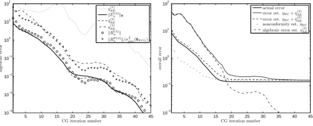
Fig. 8.2. Different errors and estimators for Example 8.1, uniformly refined mesh with 1792 elements. Left: algebraic error only; right: overall error.
5 10 15 20 25 30 35 40 45 10−4 10−3 10−2 10−1 100 101 102 CG iteration number al ge b ra ic er ro r η(1) AE kECG n kS ˆ η(2) AE η(3) AE kRCG n k kRPCG n k/σ 1 2 min(SPCG) 5 10 15 20 25 30 35 40 45 10−2 10−1 100 101 102 CG iteration number ov er al l er ro r actual error error est. ηNC+ η(3)AE error est. ηNC+ ˆη(2)AE nonconformity est. ηNC
algebraic error est. η(3) AE
Fig. 8.3. Different errors and estimators for Example 8.2 with s1 = s3 = 5, s2 = s4 = 1, adaptively refined mesh with 1812 elements. Left: algebraic error only; right: overall error.
Results for meshes obtained at the last stage of the uniform or adaptive mesh refinement process are illustrated in Figures 8.2–8.4. The results for the Laplace equation in Example 8.1 are plotted in Figure 8.2. The results for Example 8.2 with
the inhomogeneous S with si given in the left and right part of Table 8.1 are plotted
in Figure 8.3 and Figure 8.4, respectively.
Left parts of Figures 8.2–8.4 show the values of the algebraic error estimators described in Section 7, together with the true algebraic energy norm of the error
kECG
n kS (solid lines), the Euclidean norm of the algebraic residual kRCGn k (circles),
and the upper bound kRPCG
n k/σ
1/2
min(SPCG) (crosses) for kEnCGkS constructed from
the preconditioned residual, see (7.9). Please note that σmin(SPCG) is not available
and must be approximated. The true algebraic energy error kECG
n kS is evaluated by
solving SEnCG= RCGn using a direct solver. The estimator η
(1)
AE based on the weighted
norm of the algebraic residual vector, see Lemma 7.1, is plotted by dotted lines. The
estimate ˆη(2)AEevaluated for ν = 5 is plotted by dashed lines, and the estimator ηAE(3) of
Section 7.3 by dash-dotted lines.
The estimate ˆηAE(2) is close to kEkS, with some visible but insignificant
10 20 30 40 50 60 70 80 10−4 10−3 10−2 10−1 100 101 102 103 104 CG iteration number al ge b ra ic er ro r η(1) AE kECG n kS ˆ η(2) AE η(3) AE kRCG n k kRPCG n k/σ 1 2 min(SPCG) 10 20 30 40 50 60 70 80 10−1 100 101 102 CG iteration number ov er al l er ro r actual error error est. ηNC+ η(3)AE error est. ηNC+ ˆη(2)AE nonconformity est. ηNC
algebraic error est. η(3) AE
Fig. 8.4. Different errors and estimators for Example 8.2 with s1 = s3 = 100, s2 = s4 = 1, adaptively refined mesh with 1736 elements. Left: algebraic error only; right: overall error.
The estimator ηAE(3) represents a guaranteed upper bound for the algebraic error. The
estimator η(1)AE, as expected, provides the worst information among all considered
mea-sures of the algebraic error. This is in particular evident in Example 8.2 where the adaptive mesh refinement is employed, see Figures 8.3 and 8.4 (in Figure 8.4 it is out
of scale for almost all iterations). For both examples, kRCG
n k is remarkably close to
kECG
n kS. For examples of a different behavior see [46]. The upper bound constructed from the preconditioned residual is here quite tight.
On right parts of Figures 8.2–8.4 we present the actual energy (semi-)norm of
the overall error |||p − ˜pah||| (bold solid lines). We compute it in each triangle by the
7-point quadrature formula, see, e.g., [54, Section 9.10] (we consider the associated
additional error negligible). The guaranteed upper bound ηNC+ ηAE(3) on |||p − ˜pah|||
is represented by solid lines, while its components, the nonconformity estimator ηNC
and the algebraic error estimator ηAE(3), are plotted by dots and dash-dotted lines,
respectively. For comparison, we also include the estimate ηNC + ˆη(2)AE plotted by
dashed lines.
Figures 8.2–8.4 show that for small number of iterations the algebraic part of the error dominates. As the number of iterations of the conjugate gradient method grows, the algebraic part of the error drops to the level of the nonconformity error, which
is reflected by the fact that the curves of ηNC and ηAE(3) intersect. While ηNC almost
stagnates, the estimate on the algebraic error η(3)AEfurther decreases and it ultimately
gets negligible in comparison with the nonconformity error. Our stopping criteria for iterative solvers (6.1) and (6.3) essentially state that it is meaningless to continue the
algebraic computation after ηAE,K(3) (rh) ≈ γ ηNC,K is reached.
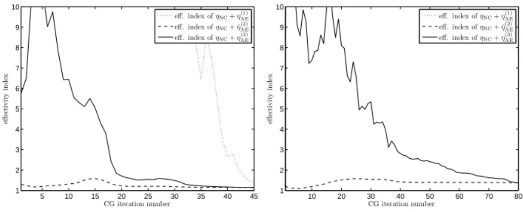
The quality of our estimates, i.e., the effectivity indices (ηNC+ ηAE)/|||p − ˜(1) pah|||
(dotted line), (ηNC+ ˆηAE)/|||p − ˜(2) pah||| (dashed line), and (ηNC+ η(3)
AE)/|||p − ˜pah||| (solid
line), is illustrated in the left part of Figure 8.5 and in Figure 8.6. Estimate η(1)AE
overestimates largely the actual algebraic error and the corresponding effectivity index is very poor (in the right part of Figure 8.6 it is completely out of scale). Recall that
the estimate ηNC+ η(3)AEgives a guaranteed upper bound. Its effectivity index is very
reasonable even in the first PCG iterations in the second case of Example 8.2. Finally,
5 10 15 20 25 30 35 1 2 3 4 5 6 7 8 9 10 CG iteration number eff ec ti v it y in d ex eff. index of ηNC+ η(1)AE eff. index of ηNC+ ˆη(2)AE eff. index of ηNC+ η(3)AE 0 500 1000 1500 2000 102 103 104 105 106 107 number of elements
condition number of the system matrix
Example 1, uniform ref. Example 2 (α=0.5354), adaptive ref. Example 2 (α=0.1269), adaptive ref.
Fig. 8.5. Effectivity indices for Example 8.1 (left), and condition number of system matrix S for Examples 8.1 and 8.2 (right).
5 10 15 20 25 30 35 40 45 1 2 3 4 5 6 7 8 9 10 CG iteration number eff ec ti v it y in d ex eff. index of ηNC+ η(1)AE eff. index of ηNC+ ˆη(2)AE eff. index of ηNC+ η(3) AE 10 20 30 40 50 60 70 80 1 2 3 4 5 6 7 8 9 10 CG iteration number eff ec ti v it y in d ex eff. index of ηNC+ η(1)AE eff. index of ηNC+ ˆη(2)AE eff. index of ηNC+ η(3) AE
Fig. 8.6. Effectivity indices for Example 8.2 with s1 = s3 = 5, s2 = s4 = 1 (left) and s1= s3= 100, s2= s4= 1 (right). The dotted line is essentially out of the scale of the figure.
ηNC + ˆη(2)AE gives in our experiments very tight estimates for the overall error. The
effectivity index is here in all cases remarkably close to one.
Without taking into consideration the algebraic part of the error, it is sometimes claimed in the literature that adaptive mesh refinement can provide an arbitrary accurate numerical solution. Similar claims should be in some cases examined and revisited. Adaptive discretization in the presence of singularity can lead to highly ill-conditioned systems of linear algebraic equations. This can have two main effects: • the iterative solvers can become slow and the computation of the numerical
solution can become expensive;
• the maximum attainable accuracy of the (direct as well as iterative) linear algebraic solvers can for highly ill-conditioned systems become very poor, which can prevent reaching the desired accuracy of the numerical solution of the original problem regardless how small the discretization error becomes. Right part of Figure 8.5 shows for our examples the dependence of the spectral condi-tion number of the system matrix S on the number of elements in the mesh. In the case of the homogeneous diffusion tensor and the uniform mesh refinement of Example 8.1, the condition number of S is growing according to the well-known theoretical result as O(N ). In Example 8.2 with inhomogeneous diffusion coefficients, adaptive mesh
refinement compensates for the effect of the singularity. This results in the growth of the condition number of the system matrix S, see the right part of Figure 8.5. If we proceed with the refinement, the condition number of S will soon reach reach the value of the inverse of machine precision, which will make algebraic computations practically meaningless. Though a more detailed discussion of this phenomenon is beyond the scope of this paper, we believe that its role can be substantial and it will have to be systematically investigated in a near future. If the conditioning of S is reasonably bounded independently of the mesh, see, e.g., [11, Section 9.6], then the matter is resolved.
9. Concluding remarks. Deriving tight a posteriori estimates under the
as-sumption that the associated systems of linear algebraic equations are solved exactly is much easier than without this assumption. It however precludes the efficient use of such estimates in practical large scale computations, where the linear systems, solved by iterative algebraic solvers, are never solved exactly, and should even be solved inexactly on purpose.
Efficient usage of iterative algebraic solvers requires balancing the algebraic and discretization errors. It is useless to make a large number of algebraic solver iterations after the algebraic error drops significantly below the discretization error. A stopping criterion must be cheap to compute. This may seem in contradiction with evaluation
of the ηNC estimator presented above, with the cost proportional to the number of
mesh elements. But ηNC does not need to be evaluated at each iteration of CG. A
viable strategy is to monitor the algebraic convergence at a negligible cost using the
algebraic error estimator ˆηAE(2) (in addition to monitoring the CG and PCG residuals),
and to evaluate any other estimators only after ˆηAE(2) drops below a certain level. The
strategy of evaluating error estimators can be tailored for a given problem in order to minimize the overall extra cost in comparison with the cost of actual computations.
If an adaptive mesh refinement leads in the presence of singularity to patholog-ically ill-conditioned linear algebraic systems, this can eventually prevent obtaining a numerical solution with a single digit of accuracy. Modeling, discretization, and computation form interconnected stages of a single solution process. As stated in [8, p. 273], “The purpose of computation is not to produce a solution with least error but to produce reliably, robustly and affordably a solution which is within a user-specified tolerance.” Therefore the errors on the different stages should be in balance, see, e.g., [44]. Considering the numerical analysis and the discretization stages separately from computations is philosophically wrong. Similar approaches will lead in solving difficult problems to dead ends.
Acknowledgments. This work was initiated during the summer school
CEM-RACS organized by the Jacques-Louis Lions laboratory (LJLL) in summer 2007 in Luminy, France and the authors gratefully acknowledge all the support. The second author thanks for the support during his visit of the LJLL in September 2008. We would also like to thank the anonymous referees for their valuable comments and suggestions.
REFERENCES
[1] Y. Achdou, C. Bernardi, and F. Coquel, A priori and a posteriori analysis of finite volume discretizations of Darcy’s equations, Numer. Math., 96 (2003), pp. 17–42.
[2] M. Ainsworth and J. T. Oden, A posteriori error estimation in finite element analysis, Pure and Applied Mathematics (New York), Wiley-Interscience [John Wiley & Sons], New York, 2000.
[3] M. Arioli, A stopping criterion for the conjugate gradient algorithm in a finite element method framework, Numer. Math., 97 (2004), pp. 1–24.
[4] M. Arioli and D. Loghin, Stopping criteria for mixed finite element problems, Electron. Trans. Numer. Anal., 29 (2007/08), pp. 178–192.
[5] M. Arioli, D. Loghin, and A. J. Wathen, Stopping criteria for iterations in finite element methods, Numer. Math., 99 (2005), pp. 381–410.
[6] I. Babuˇska, Numerical stability in problems of linear algebra, SIAM J. Numer. Anal., 9 (1972), pp. 53–77.
[7] I. Babuˇska and W. C. Rheinboldt, Error estimates for adaptive finite element computations, SIAM J. Numer. Anal., 15 (1978), pp. 736–754.
[8] B. J. C. Baxter and A. Iserles, On the foundations of computational mathematics, in Hand-book of numerical analysis, Vol. XI, Handb. Numer. Anal., XI, North-Holland, Amsterdam, 2003, pp. 3–34.
[9] R. Becker, An adaptive finite element method for the Stokes equations including control of the iteration error, in ENUMATH 97 (Heidelberg), World Sci. Publ., River Edge, NJ, 1998, pp. 609–620.
[10] R. Becker, C. Johnson, and R. Rannacher, Adaptive error control for multigrid finite element methods, Computing, 55 (1995), pp. 271–288.
[11] S. C. Brenner and L. R. Scott, The Mathematical Theory of Finite Element Methods, Texts in Applied Mathematics, Springer, 3rd ed., 2007.
[12] F. Brezzi and M. Fortin, Mixed and Hybrid Finite Element Methods, vol. 15 of Springer Series in Computational Mathematics, Springer-Verlag, New York, 1991.
[13] C. Burstedde and A. Kunoth, Fast iterative solution of elliptic control problems in wavelet discretization, J. Comput. Appl. Math., 196 (2006), pp. 299–319.
[14] D. Calvetti, S. Morigi, L. Reichel, and F. Sgallari, Computable error bounds and esti-mates for the conjugate gradient method, Numer. Algorithms, 25 (2000), pp. 75–88. Math-ematical journey through analysis, matrix theory and scientific computation (Kent, OH, 1999).
[15] P. G. Ciarlet, The Finite Element Method for Elliptic Problems, vol. 4 of Studies in Mathe-matics and its Applications, North-Holland, Amsterdam, 1978.
[16] P. Deuflhard, Cascadic conjugate gradient methods for elliptic partial differential equations: algorithm and numerical results, in Domain decomposition methods in scientific and engi-neering computing (University Park, PA, 1993), vol. 180 of Contemp. Math., Amer. Math. Soc., Providence, RI, 1994, pp. 29–42.
[17] R. Eymard, T. Gallou¨et, and R. Herbin, Finite volume methods, in Handbook of Numerical Analysis, Vol. VII, North-Holland, Amsterdam, 2000, pp. 713–1020.
[18] G. H. Golub and G. Meurant, Matrices, moments and quadrature, in Numerical analysis 1993 (Dundee, 1993), vol. 303 of Pitman Res. Notes Math. Ser., Longman Sci. Tech., Harlow, 1994, pp. 105–156.
[19] G. H. Golub and G. Meurant, Matrices, moments and quadrature II: how to compute the norm of the error in iterative methods, BIT, 37 (1997), pp. 687–705.
[20] G. H. Golub and Z. Strakoˇs, Estimates in quadratic formulas, Numer. Algorithms, 8 (1994), pp. 241–268.
[21] M. R. Hestenes and E. Stiefel, Methods of conjugate gradients for solving linear systems, J. Res. Natl. Bur. Stand., 49 (1952), pp. 409–436.
[22] N. J. Higham, Accuracy and Stability of Numerical Algorithms, Society for Industrial and Applied Mathematics (SIAM), Philadelphia, PA, second ed., 2002.
[23] K. Y. Kim, A posteriori error analysis for locally conservative mixed methods, Math. Comp., 76 (2007), pp. 43–66.
[24] Y. Maday and A. T. Patera, Numerical analysis of a posteriori finite element bounds for linear functional outputs, Math. Models Methods Appl. Sci., 10 (2000), pp. 785–799. [25] D. Meidner, R. Rannacher, and J. Vihharev, Goal-oriented error control of the iterative
solution of finite element equations, J. Numer. Math., 17 (2009), pp. 143–172.
[26] J. A. Meijerink and H. A. van der Vorst, An iterative solution method for linear systems of which the coefficient matrix is a symmetric M-matrix, Math. Comp., 31 (1977), pp. 148– 162.
[27] G. Meurant, The computation of bounds for the norm of the error in the conjugate gradient algorithm, Numer. Algorithms, 16 (1997), pp. 77–87.